Article

Dynamic Modeling and Response Analysis of Dielectric Elastomer Incorporating Fractional Viscoelasticity and Gent Function

1
School of Mathematics and Statistics, Taiyuan Normal University, Taiyuan 030619, China
2
Department of Applied Mathematics, Northwestern Polytechnical University, Xi’an 710129, China
*
Author to whom correspondence should be addressed.
Fractal Fract. 2023, 7(11), 786; https://doi.org/10.3390/fractalfract7110786
Submission received: 6 September 2023 / Revised: 2 October 2023 / Accepted: 3 October 2023 / Published: 28 October 2023

Abstract

:
Dielectric Elastomer (DE) has been recognized for its remarkable potential in actuation and sensing applications. However, the functionality of most DE materials is restricted by their high viscoelastic effects. Currently, there is a lack of dynamic models that consider both viscoelasticity and stiffening effects. To address this research gap, we propose a fractional-order model in this study. Specifically, the model comprehensively integrates both viscoelastic and stiffening effects under electromechanical coupling, utilizing the principle of virtual work. Further, the effects of the system parameters are analyzed. The results indicate that the fractional-order derivative influences the hysteresis behaviors during the transient state and affects the duration of the transient process. Furthermore, when the system’s energy surpasses a certain threshold, the steady-state response can transition between two distinct potential wells. Through the manipulation of electromechanical coupling parameters, bifurcation can be induced, and the occurrence of snap-through and snap-back behaviors can be controlled. These findings have significant implications for the design and optimization of DE materials in various applications.

1. Introduction

As a new smart material, DE has garnered significant attention owing to its unique attributes, including remarkable deformability, rapid responsiveness, light weight, highly efficient electromechanical conversion, and robust environmental adaptability. These distinctive attributes have led to its extensive application in diverse domains, such as artificial intelligence, aerospace, bio-simulation mechanisms, and bio-medicine [1,2,3,4,5,6,7].
The concept of electromechanical coupling in DE was first proposed by Stark and Garton [8]. Since then, numerous studies have been conducted to explore the behaviors of DE under electromechanical coupling both experimentally and theoretically [9,10,11,12,13]. Due to the potential applications of DE materials, a comprehensive analysis of inertia’s impact on their dynamic performance is essential [14,15]. For instance, Zhu et al. conducted a theoretical analysis of the nonlinear oscillation of DE balloons, delving into the parametric responses [16]. Son et al. developed a dynamic model of tubular DE transducers, utilizing the finite difference method to explore dynamic responses [17]. Yong et al. focused on the nonlinear vibration response of thick spherical shells, analyzing their dynamic behaviors and deriving the critical voltage [18]. Yin et al. performed a nonlinear dynamic analysis and scrutinized the effects of electrostriction on free oscillation and parametric excitation [19]. However, the majority of these investigations primarily focused on small stable stretches.
The emergence of Very High Bond (VHB) material has revolutionized the deformation scale of DE materials, as is widely known [20]. Numerous experiments have consistently demonstrated that DE exhibits strain-stiffening under large deformations [21,22,23,24]. As a result, any analysis of DE behaviors must inherently account for the impact of strain-stiffening [25,26]. Wang et al. were pioneers in developing a theoretical model and investigating the effect of strain-stiffening on the dynamic characteristics of a circular DE membranes [27]. However, Wang did not incorporate viscoelastic damping into the model. Subsequently, Lv et al. proposed a model that encompassed both stiffening and damping effects, analyzing the dynamic performance [28]. Nevertheless, Lv only characterized the viscoelastic effect as a damping force, which fell short of fully capturing the significant viscoelasticity inherent to DE. Hence, there is still a need for further research to delve into the combined impact of viscoelasticity and strain-stiffening on the dynamic responses of DE materials.
Substantial experimental studies have shown that under electromechanical coupling, the response of DE is highly rate-dependent, indicating that DE materials possess significant viscoelastic properties [20,29]. However, such rate-dependence can result in application failures and reduced coupling efficiency [30,31]. As a result, many scholars have focused on developing viscoelastic models for DE. For example, Yang et al. established a nonlinear viscoelastic model for finite deformations using Christensen’s viscoelastic theory [32]. Hong and Foo et al. adopted a rheological model featuring two parallel elements to characterize viscoelasticity while investigating dynamic response and hysteresis behaviors [33,34]. Afterwards, Zhang et al. utilized a combined Kelvin–Voigt–Maxwell model to describe the viscoelastic behavior, although they did not examine the performance of DE [35]. Later, Somayeh et al. derived fractional and non-fractional viscoelastic models for DE [36]. Moreover, the fractional Kelvin–Voigt model was employed to determine the elastic and/or viscous material properties. However, its applicability is confined to small strain states [37,38]. Given the significant viscoelasticity of DE, a viscoelastic model that integrates infinite elastic and viscous elements is highly sought after. Hence, the pursuit of the most superior viscoelastic model remains a crucial research area. In this paper, we propose to modify the characterization of viscoelasticity by using the fractional-order dashpot model. In the literature [39,40], such an element is called a Scott–Blair element and is graphically represented by a rhombus.
Extensive research has been conducted in the field of solving fractional order differential equations leading to the development of various numerical techniques. These methods encompass Adomian’s decomposition method [41], the Homotopy perturbation method [42], method of discretization approximation [43,44], finite element analysis [45], etc.
Despite recent advancements on DE, there are a limited number of modeling works regarding the dynamic response of DE. This is especially noticeable when considering the strain-stiffening effect and viscoelasticity. These intricate behaviors exhibited by DE materials present substantial challenges for modeling endeavors. To bridge this research gap, this paper proposes a dynamic model that comprehensively incorporates both the strain-stiffening effect and viscoelasticity. The aim of using this model is to investigate the dynamic response of DE under electromechanical coupling loading. This paper is structured as follows: In Section 2, the governing equation is derived utilizing the method of virtual work. In Section 3, an investigation is conducted to examine the influence of fractional order and electromechanical coupling parameters on the response of circular DE. Finally, we present our conclusions. To summarize, this paper provides a innovative approach for modeling the dynamic response of DE, encompassing both strain-stiffening and viscoelasticity. By investigating the impact of fractional order and electromechanical coupling parameters on circular DE’s response, this study offers invaluable insights pertinent the design and optimization of DE-based devices.

2. Governing Equation Incorporating Stiffening and Viscoelasticity

Here, we consider a circular DE membrane that has two compliant electrodes on each surface. When subjected to voltage Φ and radial force P, the DE membrane undergoes compression in its thickness while expanding its surface area. The behavior is depicted in Figure 1. Taking into account the assumption of incompressibility, the stretch ratio and the deformation thickness are defined as λ ( t ) = r ( t ) / R and h ( t ) = H / λ 2 ( t ) , respectively. The electric displacement is expressed as D t = Q t / π r 2 t = Q t / π R 2 λ 2 t .

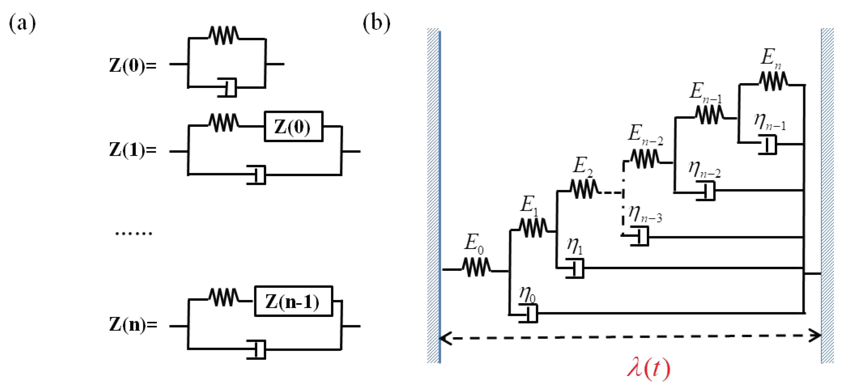
2.1. A Fractional Model of Viscoelastic Behavior of DE

Despite the promising potential applications of DE, the remarkable viscoelastic behavior inherent in DE has affected both the electromechanical coupling efficiency and deformation stability. Consequently, researchers have made efforts to investigate viscoelastic behavior from various approaches, which has led to the establishment and utilization of several models.
As is shown in Figure 2a, Z(0) represents the Voigt–Kelvin model, which is adept at capturing creep behavior. However, it does not provide an accurate depiction of stress relaxation in viscoelastic materials. To account for the relaxation phenomenon, some ideas similar to the Maxwell model are invoked. Subsequently, the elastic elements from the initial parallel unit of Z(0) are serially connected with Z(0), resulting in the emergence of Z(1). Next, an iterative approach is adopted to elevate the complexity of element amalgamation, while considering the indistinguishability among viscoelastic phenomena. Consequently, as the number of iterations increases, the representation of DE’s viscoelastic behavior becomes progressively more precise. The general term of iteration is displayed by Z(n) in Figure 2a. In order to incorporate the initial elastic strain within the DE material, a spring element is introduced in a series with Z(n), resulting in the composite element shown in Figure 2b.
In this paper, Figure 2b represents the schematic diagram of the DE viscoelastic model. By adopting the solution approach outlined in paper [46], a fractional order dashpot model can be obtained as the number of iterations n of Z(n) approaches infinity.
For simplicity, at time t, the viscoelastic stress σ can be characterized as follows:
σ = η D q λ t ,
where η = E 0 k q (Pa q ), E 0 means the Modulus of elasticity (Pa), k = η 0 / E 0 expresses the relaxation time(s), q is the fractional order indicating the degree of viscoelasticity of materials, and D q λ ( t ) denotes the fractional-order derivative under the definition of Riemann–Liouville,
D q λ ( t ) = 1 Γ 1 q d d t 0 t λ t τ τ q d τ , 0 < q < 1 .
Then, the curves depicting stress relaxation and creep behavior are shown in Figure 3. Similar to the practical deformation process of DE, these curves exhibit the nonlinear trajectory when the fractional order q falls within the open interval ( 0 , 1 ) . This observation further indicates the compatibility of the fractional model with the viscoelastic characteristics of DE.

2.2. The Method of Virtual Work

Without loss of generality, the combination of the voltage Φ , the radial force P and DE membrane constitutes a thermodynamic system operating under isothermal conditions. By employing the method of virtual work applicable to the thermodynamic systems, the equations can be readily derived as follows:
π R 2 H δ W = W v o l + W r f + W i f + W σ , W v o l = Φ δ Q = Φ δ π r 2 D , W r f = P δ 2 π r , W i f = F δ r = ρ V d 2 r / d t 2 δ r , W σ = σ δ 2 π r ,
where W denotes the density of Helmholtz free energy. W v o l , W r f , W i f , and W σ correspond to the work carried out by voltage Φ , radial force P, inertial force F, and viscoelastic stress σ , respectively. ρ and V indicate the density and volume of the DE material. Moreover, the density of Helmholtz free energy is derived by adding the elastic energy as well as the dielectric energy:
W = μ J lim 2 ln 1 2 λ 2 + λ 4 3 J lim + D 2 2 ε ,
referring to articles [27,28], hyper-elastic Gent model can be applied to characterize strain-stiffening effect. Here, μ indicates the shear modulus, ε means the permittivity of DE, J lim denotes the constant related to limit stretch and can be taken as J lim = 100 . By combining Equation (2) with (3), and eliminating D, a governing equation involving a single variable can be obtained:
d 2 λ d T 2 + c D q λ + g S f , S , λ = 0 ,
with
g S f , S , λ = S f λ 3 S + λ λ 5 1 2 λ 2 + λ 4 3 J lim ,
where T = t / R ρ / 2 μ is the dimensionless time, c = η 1 / R ρ / 2 μ q / μ R H expresses the viscoelastic damping coefficient, S f = ε Φ 2 / μ H 2 and S = P / μ R H denote the electromechanical coupling parameters as functions of the voltage and the radial force, respectively.

3. Nonlinear Dynamic Analysis of DE with Fractional Damping

For general differential equations, they can be transformed into integral equations, providing an avenue for solving the original equation. This approach is also applicable to numerical solutions for fractional derivative equations, with the prediction correction method being the most commonly employed.
Many practical issues in life can be mathematically modeled using appropriate differential equation models. The solution of differential equations is no longer limited to the pursuit of exact solutions but has expanded to include numerical algorithm solutions. Fractional-order differential equations have gained significant attention and development in various research areas, owing to their enhanced ability to accurately model certain system processes. However, the introduction of fractional orders into models increases system complexity and may hinder computational efficiency, potentially requiring prolonged computation times or resulting in significant deviations in results due to precision issues. In this paper, an effective algorithm proposed by Chen [44] is employed to transform fractional-order systems into integer-order systems, enabling rapid and high-precision simulation of fractional-order calculus systems.
The system (4) can be transformed into a first-order derivative form:
X 1 = λ , d X 1 d t = X 2 , d X 2 d t = S f X 1 3 S + X 1 X 1 5 1 2 X 1 2 + X 1 4 3 J lim c 1 Γ 1 q X 1 0 t q + sin π q π i = 1 n ω i n φ 2 x i n 1 x i n , t 1 x i n 1 x i n , d φ 2 y i n , t d t = y i n 2 q 1 X 2 t y i n 2 φ 2 y i n , t .
Here,
x i n = cos 2 2 i 1 π 4 n + 2 , ω i n = 2 π 2 n + 1 cos 2 2 i 1 π 4 n + 2 , y i n = x i n 1 x i n , X 1 0 = X 10 , X 2 0 = X 20 , φ 2 y i n , 0 = 0 .
In simulation, select i = 6 and use the fourth order Runge–Kutta method to obtain response statistics (with a time step of 0.0005).
In the subsequent part of this section, we analyze dynamic response using some ideas and data in [27].

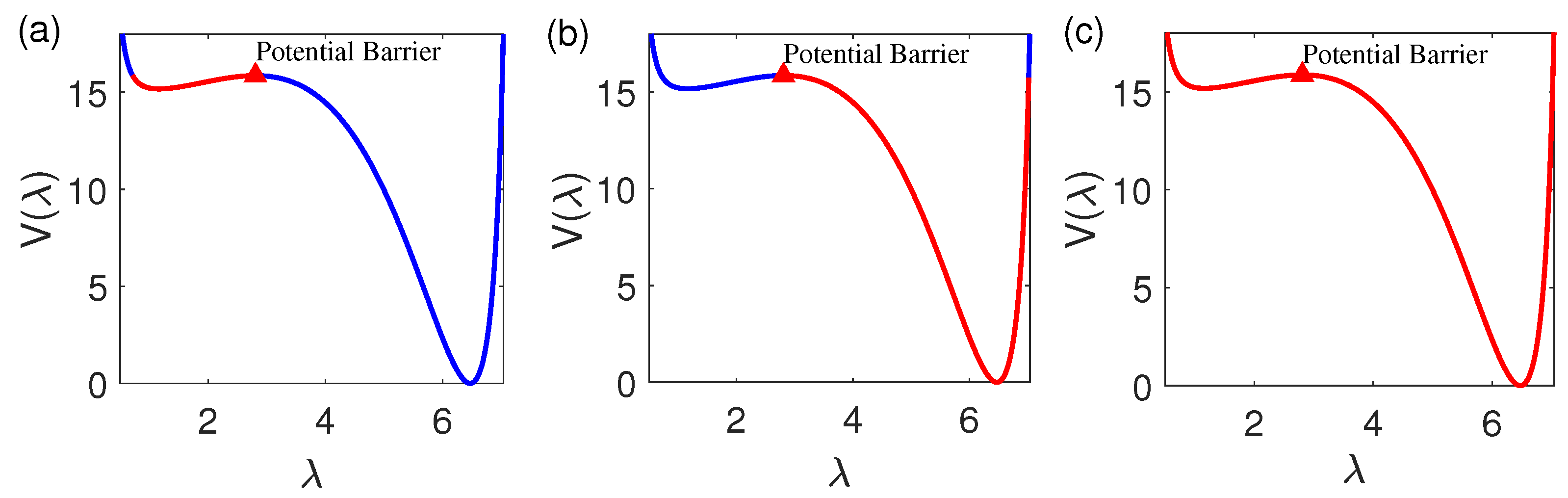
3.1. Preliminary Study of System Response Using the Potential Function

Generally speaking, a potential well corresponds to a stable state. Thus, the response of DE system can be initially analyzed preliminarily using the potential function V ( λ ) . Considering the complexity of nonlinear integral equation, the type diagram depicting stable states is obtained numerically through the application of zero-point judgment theory, as shown in Figure 4. Obviously, two stable modes are exhibited on the S S f plane: monostable state and bistable state. Moreover, fine-tuning the electromechanical parameters enables the manipulation of the shift between these two stable states. This implies that, the active morphology of DE can be regulated by applying the electromechanical load.

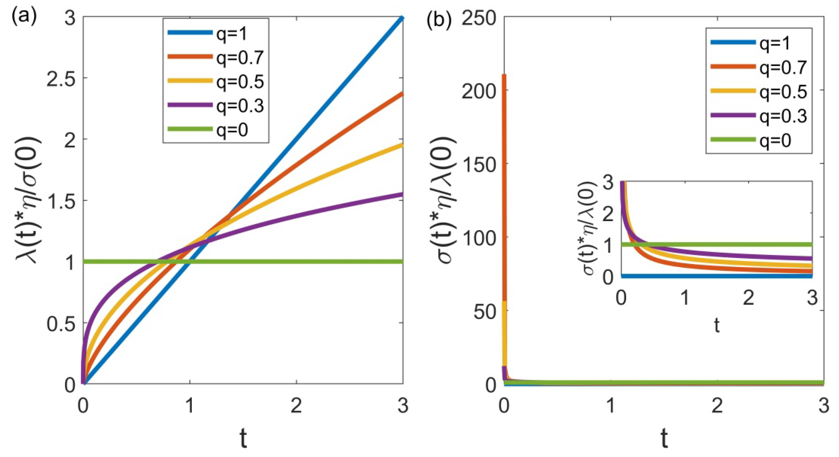
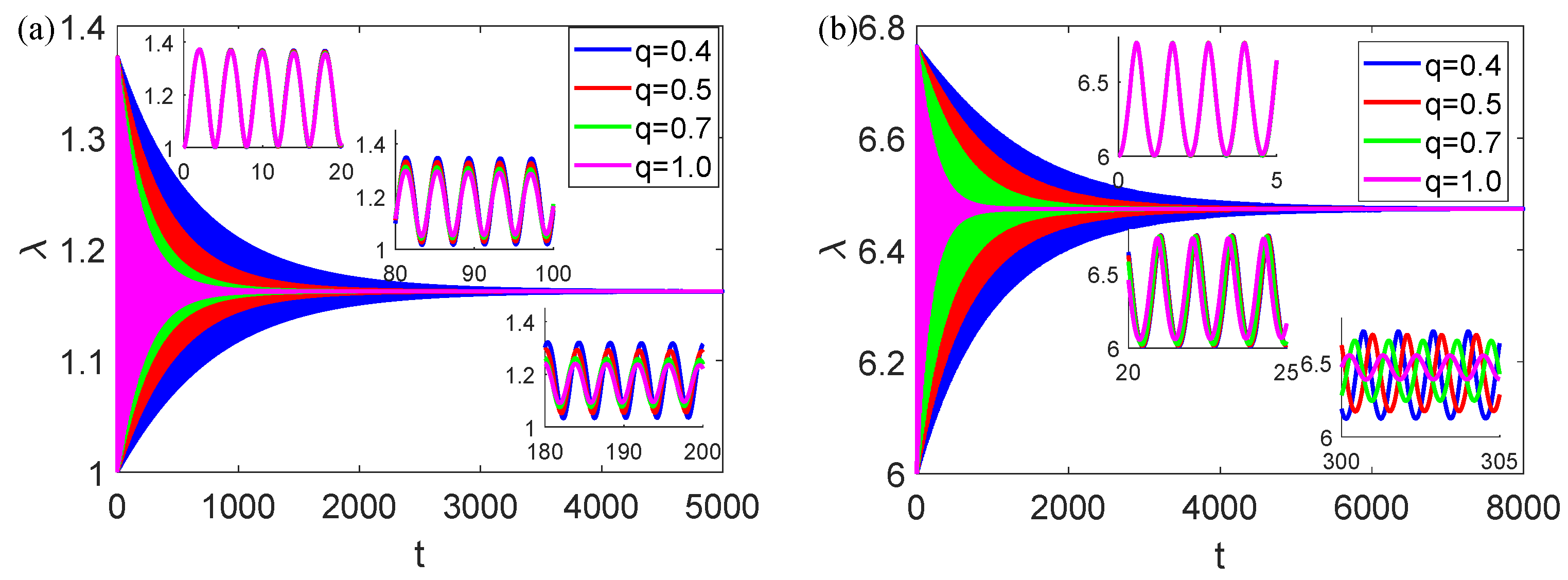
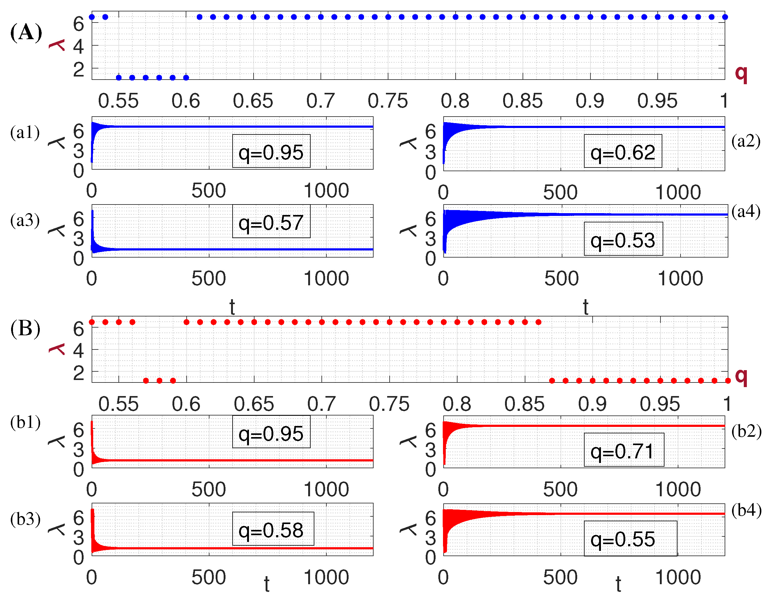
3.2. The Effect of Fractional Derivative on System

In this subsection, the effect of fractional derivative on system’s dynamics is investigated in detail. Here, we mainly focus on bistability with fixed the electromechanical parameters set as follows: S f = 0.35 2 and S = 0.5 as shown in Figure 4. Then, two stable equilibrium stretch ratio are determined, λ l 1.1622 and λ r 6.4733 . Additionally, an unstable equilibrium point is present at approximately λ e q _ u n s t a b l e 2.8086 . Herein, the viscoelasticity damping coefficient is defined as c = 0.01 . Consequently, we observe the existence of two attractors, and if the system’s initial conditions lie within the basin of attraction, it will evolve and ultimately converge to respective attractor. Moreover, Figure 5 depicts the three distinct motion patterns of the DE system: oscillations in the left-side well, oscillations in the right-side well, and transition between the two wells. Notably, oscillations are restricted in a single basin of attraction in Figure 5a,b. For clarity in distinguishing oscillatory behaviors, denoting λ l 1.1622 and λ r 6.4733 correspond to the positions of first and the second steady-state position of DE, respectively. Moreover, Figure 5c exhibits oscillations from one well to the other. And the critical condition for achieving this transition is to satisfy the inequality E 0 > E b a r r i e r . Here, the initial energy E 0 = V λ 0 + λ ˙ 0 2 / 2 , where V denotes the potential function. Additionally, E b a r r i e r = V λ e q _ u n s t a b l e is defined as the energy of potential barrier. In the following, we divide investigations into two parts to explore the impact of fractional derivative on response of DE system. The first part focuses on oscillations within a single potential well, i.e., E 0 < E b a r r i e r . The second part examines oscillations transitioning between two potential wells, i.e., E 0 > E b a r r i e r .

3.2.1. Oscillation in the Single Potential Well

Based on the above analyses, we can deduce that, if λ 0 < λ e q _ u n s t a b l e , the initial position corresponds to the left-side well; otherwise, it corresponds to the right-side well. Thus, we set the initial conditions as λ 0 = 1 and λ 0 = 6 to explore both potential wells. Additionally, we choose λ ˙ ( 0 ) = 0 , ensuring that the inequality E 0 < E b a r r i e r is satisfied. Next, the results are shown in Figure 6.
From Figure 6a, it is observed that the increasing fractional order leads to shorter transient times. A fact is that, in DE materials, the larger fractional order corresponds to stronger viscosity. Consequently, greater DE viscosity results in reduced oscillation amplitude and duration. Next, we delve into the details by analyzing inset figures in Figure 6a. Remarkably, within [ 0 , 20 ] , the time series curves graphs corresponding to different fractional orders coincide each other. Namely, in a short time, the effect of viscoelasticity is unconspicuous. As the time variable shifts to the interval [ 80 , 100 ] , amplitudes of response curves becomes asynchronous. Subsequently, phase asynchrony in the response becomes apparent during the time interval [ 180 , 200 ] . That is, viscoelastic behavior evolves gradually from amplitude to phase. Notably, the inset figures in Figure 6b demonstrate a shorter duration of curves coincidence, compared to those in Figure 6a. Furthermore, in right-side oscillation, viscoelastic behavior transitions directly from the coincidence state to unsynchronized state in both amplitude and phase. In other words, the viscoelasticity of DE exhibits greater sensitivity to the second steady-state position than the first.

3.2.2. Oscillation between Two Potential Wells

Similarly, we consider two initial positions: λ 0 = 1 and λ 0 = 5 . Ensuring the condition E 0 > E b a r r i e r , the rates of stretch ratio can be set as: λ ˙ 0 = 2 and λ ˙ 0 = 4 . The dynamic behaviors of DE material are illustrated below. As depicted in Figure 7A, when q is fixed, the λ e q is determined. λ e q can exist either in the initial potential well or during the transition to the other well. This implies that the viscoelasticity of DE material can induce a shift in the steady-state positions. Furthermore, upon analyzing Figure 7A,B, it becomes evident that a larger fractional derivative corresponds to a higher transition probability between the two wells. In other words, for DE material, greater viscosity makes it easier to shift the steady-state positions. Subsequently, Figure 7(a1–a4),(b1–b4) show the response behaviors with time under the fixed fractional derivative q. From these figures, significant amplitude oscillations between the two wells are observed during the transient process. That indicates that, higher initial energy leads to larger amplitude oscillations.

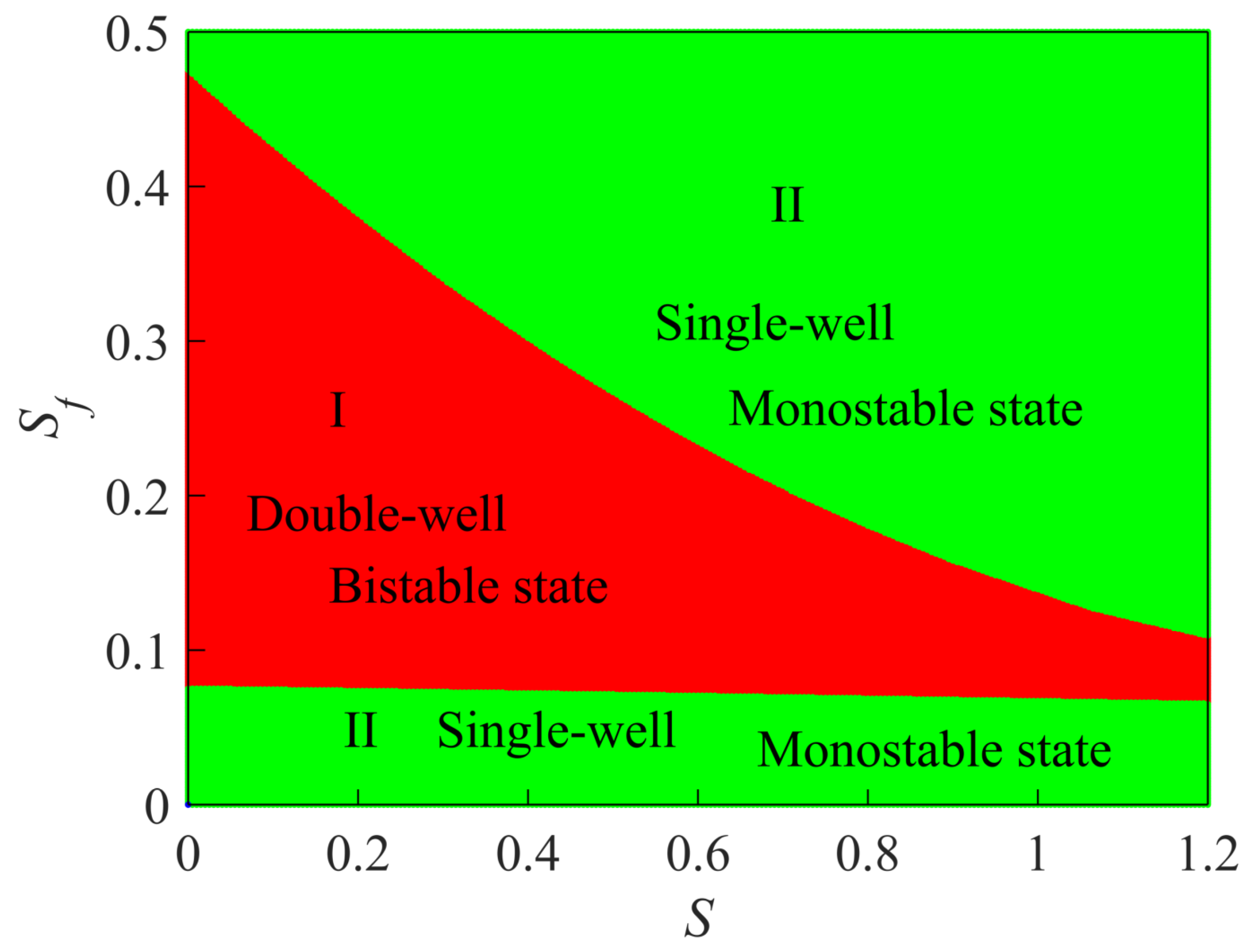
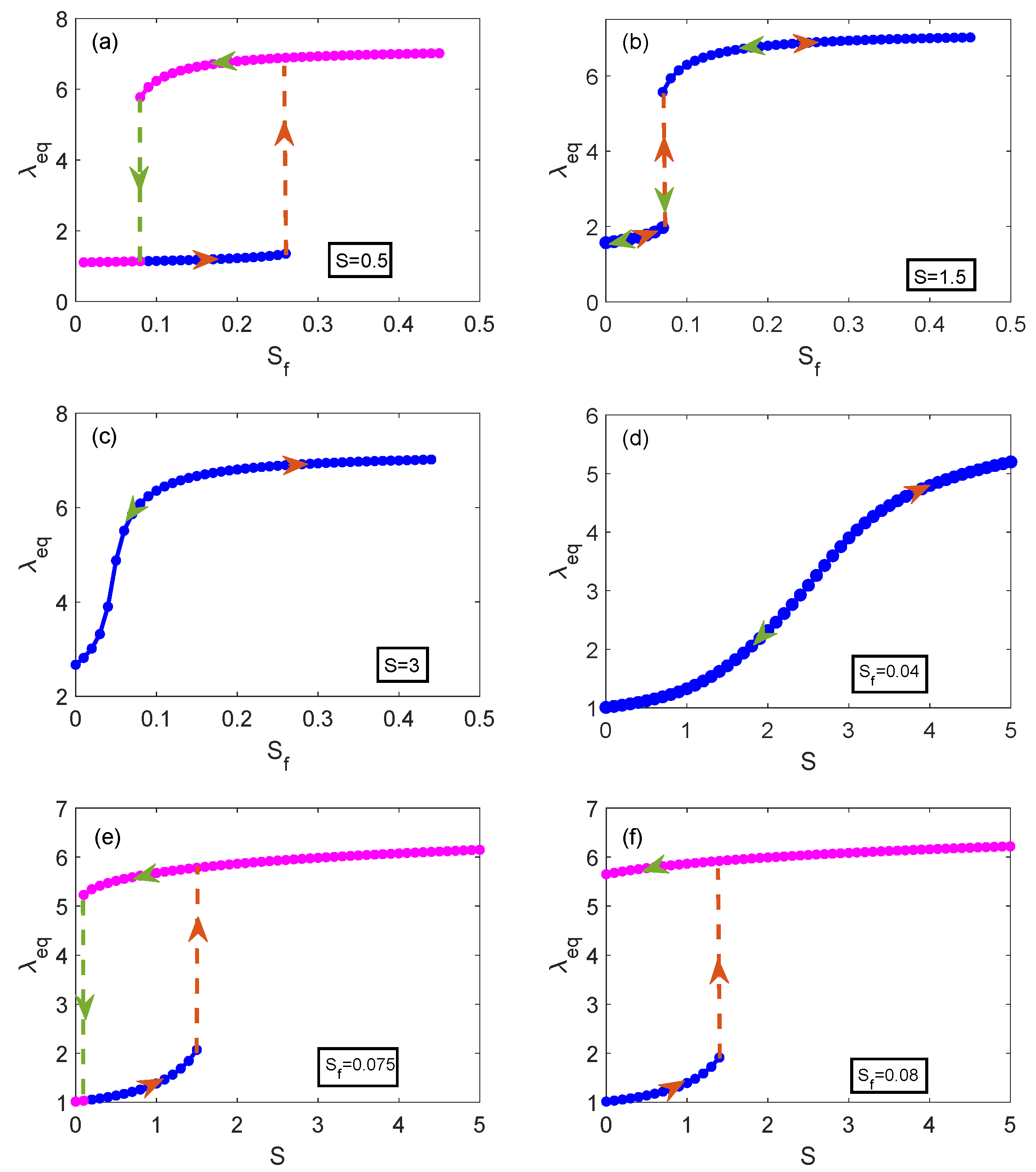
3.2.3. The Effect of Electromechanical Coupling Parameters on the Response of Equilibrium State

When λ ˙ 0 is small, i.e., when E 0 < E b a r r i e r , the effect of fractional order derivative on the steady-state response is almost negligible. In view of this, the relation between equilibrium stretch ratio and electromechanical coupling parameters is studied based on a fixed fractional-order derivative. Here, q = 0.9 . Figure 8a–c make plots of the equilibrium stretch ratio λ e q as a function of voltage parameter for three values of the radial force. For radial force S = 0.5 (Figure 8a), with the increasing of voltage S f , the λ e q increases gradually, until the S f climbs to S f = 0.26 , the λ e q suddenly jumps discontinuously, and then, with the further increase in the S f , the λ e q increases monotonously. Moreover, when the S f decreases, the λ e q reduces and suddenly falls discontinuously at S f = 0.08 , later, λ e q gradually decreases with the continuous decrease in S f . Namely, for DE material, the phenomena of snap-through and snap-back occur with the change of voltage. Most interestingly, the two positions of sudden jump are different. That is, a hysteresis loop is presented obviously between S f = 0.08 and S f = 0.26 . When S = 1.5 (Figure 8b), the snap-through and snap-back behaviors still exist, whereas the hysteresis loop vanishes. So, the larger the S, the narrower the hysteresis loop. Furthermore, a larger radial force is provided in Figure 8c ( S = 3 ), the above behaviors of snap-through and snap-back disappear, and the λ e q changes progressively. Therefore, increasing the S f can achieve enhancement of the λ e q . Not only that, the behaviors of the snap-through and snap-back can also be controlled by adjusting the S. Moreover, we can also carry out the same analysis for the relation curves of radial force and the equilibrium stretch λ e q under different value of voltage (Figure 8d–f). When the voltage is fixed at 0.04 (Figure 8d), the λ e q changes in the S monotonously. That is, the process of stretch of DE is stable. For S f = 0.075 (Figure 8e), the snap-through and snap-back appear at S = 1.5 and S = 0.1 , respectively. Namely, a hysteresis loop is presented with the increasing of the S f . In addition, the bistability could be induced, when the S f increases. Furthermore, the continuous increases of S f , an interesting phenomenon is noticed (Figure 8f). With the increases of S, the λ e q sudden jump, however, the sudden jump disappeared in process of the decreasing of S. That is, the snap-back behavior is destroyed. Hence, the snap-through cannot coexist with snap-back when the voltage is too high or too low. And the phenomena of snap-through and snap-back can be avoided under lower voltage.

4. Conclusions

Utilizing iterative methods, a better interpretation of the complex viscoelastic behavior of polymer materials is provided. Building upon this, a fractional-order model is employed. Moreover, a dynamic model of DE is formulated, considering both the strain-stiffening effect and viscoelasticity effects within electromechanical coupling. Subsequently, the model’s dynamic response is investigated in relation to the fractional order derivative and the electromechanical coupling parameters. The findings indicate that viscoelasticity can trigger transitions between two equilibrium positions under specific inequality conditions. Additionally, an increase in viscosity can induce a decrease in oscillation amplitude and duration. Moreover, increased viscosity is more prone to causing shifts in steady-state positions. The electromechanical parameters determine not only the system’s stability mode (monostability or bistability) but also influence the equilibrium point of the strain ratio. Furthermore, manipulation of the electromechanical parameters can either hinder or prompt snap-through and snap-back behaviors. In some cases, a hysteresis loop can be occasionally observed. The objective of this paper is to provide guidance for theoretical modeling and broaden the practical applications of DE materials.

Author Contributions

Conceptualization, Q.L. and Z.S.; methodology, Z.S. and Q.L.; software and validation, Q.L.; writing—original draft preparation, Q.L.; supervision, Z.S. All authors have read and agreed to the published version of the manuscript.

Funding

This work was supported by the National Natural Science Foundation of China (Grant Nos. 11972288, 12272295). The authors would like to thank the anonymous referees for their efforts and valuable comments.

Data Availability Statement

Not applicable.

Conflicts of Interest
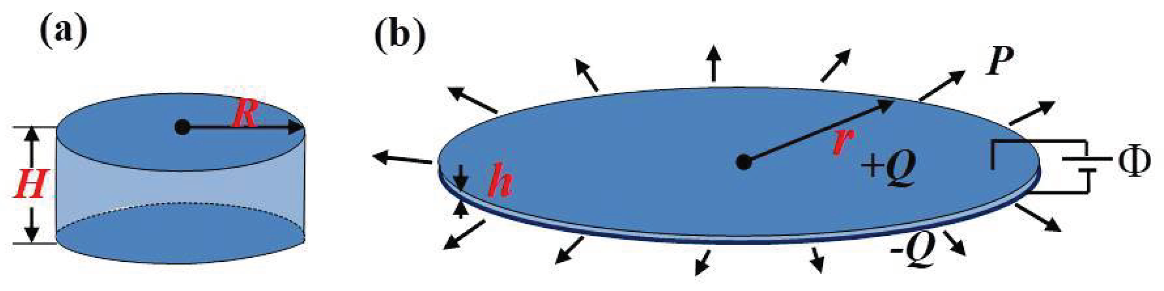
The authors declare no conflict of interest.

Notation

In the present paper, for the convenience of the readers, we will use the following notations.
Φ voltage (kV)
Pradial force (N)
λ t stretch ratio at time t
r t radius at time t (mm)
h t thickness at time t (mm)
D t electric displacement at time t
Q t the charges of polarity carried on surface at time t
σ viscoelastic stress
Wthe density of Helmholtz free energy
W v o l the work carried out by the voltage
W r f the work carried out by the radial force
W i f the work carried out by the inertial force
W σ the work carried out by the viscoelastic stress

References

  1. Anderson, I.A.; Gisby, T.A.; McKay, T.G.; O’Brien, B.M.; Calius, E.P. Multi-functional dielectric elastomer artificial muscles for soft and smart machines. J. Appl. Phys. 2012, 112, 041101. [Google Scholar] [CrossRef]
  2. Henke, E.F.M.; Schlatter, S.; Anderson, I.A. Soft dielectric elastomer oscillators driving bioinspired robots. Soft Robot. 2017, 4, 353–366. [Google Scholar] [CrossRef] [PubMed]
  3. Shintake, J.; Cacucciolo, V.; Shea, H.; Floreano, D. Soft biomimetic fish robot made of dielectric elastomer actuators. Soft Robot. 2018, 5, 466–474. [Google Scholar] [CrossRef] [PubMed]
  4. Zhao, J.; Niu, J.; McCoul, D.; Ren, Z.; Pei, Q. Phenomena of nonlinear oscillation and special resonance of a dielectric elastomer minimum energy structure rotary joint. Appl. Phys. Lett. 2015, 106, 133504. [Google Scholar] [CrossRef]
  5. O’Brien, B.M.; Calius, E.P.; Inamura, T.; Xie, S.Q.; Anderson, I.A. Dielectric elastomer switches for smart artificial muscles. Appl. Phys. A 2010, 100, 385–389. [Google Scholar] [CrossRef]
  6. Kornbluh, R.D.; Pelrine, R.; Pei, Q.; Heydt, R.; Stanford, S.; Oh, S.; Eckerle, J. Electroelastomers: Applications of dielectric elastomer transducers for actuation, generation, and smart structures. In Proceedings of the SPIE’s 9th Annual International Symposium on Smart Structures and Materials, San Diego, CA, USA, 17–21 March 2002; Volume 4698, pp. 254–270. [Google Scholar]
  7. Pei, Q.; Pelrine, R.; Stanford, S.; Kornbluh, R.; Rosenthal, M. Electroelastomer rolls and their application for biomimetic walking robots. Synth. Met. 2003, 135, 129–131. [Google Scholar] [CrossRef]
  8. Stark, K.; Garton, C. Electric strength of irradiated polythene. Nature 1955, 176, 1225–1226. [Google Scholar] [CrossRef]
  9. Guo, Y.; Liu, L.; Liu, Y.; Leng, J. Review of Dielectric Elastomer Actuators and Their Applications in Soft Robots. Adv. Intell. Syst. 2021, 3, 2000282. [Google Scholar] [CrossRef]
  10. Cao, C.; Chen, L.; Hill, T.L.; Wang, L.; Gao, X. Exploiting Bistability for High-Performance Dielectric Elastomer Resonators. IEEE/ASME Trans. Mechatron. 2022, 27, 5994–6005. [Google Scholar] [CrossRef]
  11. Liu, N.; Martinez, T.; Walter, A.; Civet, Y.; Perriard, Y. Control-Oriented Modeling and Analysis of Tubular Dielectric Elastomer Actuators Dedicated to Cardiac Assist Devices. IEEE Robot. Autom. Lett. 2022, 7, 4361–4367. [Google Scholar] [CrossRef]
  12. Acome, E.; Mitchell, S.K.; Morrissey, T.G.; Emmett, M.B.; Benjamin, C.; King, M.; Radakovitz, M.; Keplinger, C. Hydraulically amplified self-healing electrostatic actuators with muscle-like performance. Science 2018, 359, 61–65. [Google Scholar] [CrossRef] [PubMed]
  13. Cacucciolo, V.; Shintake, J.; Kuwajima, Y.; Maeda, S.; Floreano, D.; Shea, H. Stretchable pumps for soft machines. Nature 2019, 572, 516–519. [Google Scholar] [CrossRef] [PubMed]
  14. Mockensturm, E.M.; Goulbourne, N. Dynamic response of dielectric elastomers. Int. J. Non-Linear Mech. 2006, 41, 388–395. [Google Scholar] [CrossRef]
  15. Fox, J.; Goulbourne, N. On the dynamic electromechanical loading of dielectric elastomer membranes. J. Mech. Phys. Solids 2008, 56, 2669–2686. [Google Scholar] [CrossRef]
  16. Zhu, J.; Cai, S.; Suo, Z. Nonlinear oscillation of a dielectric elastomer balloon. Polym. Int. 2010, 59, 378–383. [Google Scholar] [CrossRef]
  17. Son, S.; Goulbourne, N. Dynamic response of tubular dielectric elastomer transducers. Int. J. Solids Struct. 2010, 47, 2672–2679. [Google Scholar] [CrossRef]
  18. Yong, H.; He, X.; Zhou, Y. Dynamics of a thick-walled dielectric elastomer spherical shell. Int. J. Eng. Sci. 2011, 49, 792–800. [Google Scholar] [CrossRef]
  19. Yin, Y.; Zhao, D.; Liu, J.; Xu, Z. Nonlinear dynamic analysis of dielectric elastomer membrane with electrostriction. Appl. Math. Mech. 2022, 43, 793–812. [Google Scholar] [CrossRef]
  20. Pelrine, R.; Kornbluh, R.; Pei, Q.; Joseph, J. High-speed electrically actuated elastomers with strain greater than 100%. Science 2000, 287, 836–839. [Google Scholar] [CrossRef]
  21. An, L.; Wang, F.; Cheng, S.; Lu, T.; Wang, T. Experimental investigation of the electromechanical phase transition in a dielectric elastomer tube. Smart Mater. Struct. 2015, 24, 035006. [Google Scholar] [CrossRef]
  22. Keplinger, C.; Li, T.; Baumgartner, R.; Suo, Z.; Bauer, S. Harnessing snap-through instability in soft dielectrics to achieve giant voltage-triggered deformation. Soft Matter 2012, 8, 285–288. [Google Scholar] [CrossRef]
  23. Li, T.; Keplinger, C.; Baumgartner, R.; Bauer, S.; Yang, W.; Suo, Z. Giant voltage-induced deformation in dielectric elastomers near the verge of snap-through instability. J. Mech. Phys. Solids 2013, 61, 611–628. [Google Scholar] [CrossRef]
  24. Lu, T.Q.; Suo, Z.G. Large conversion of energy in dielectric elastomers by electromechanical phase transition. Acta Mech. Sin. 2012, 28, 1106–1114. [Google Scholar] [CrossRef]
  25. Zhao, X.; Hong, W.; Suo, Z. Electromechanical hysteresis and coexistent states in dielectric elastomers. Phys. Rev. B 2007, 76, 134113. [Google Scholar] [CrossRef]
  26. Zhou, J.; Hong, W.; Zhao, X.; Zhang, Z.; Suo, Z. Propagation of instability in dielectric elastomers. Int. J. Solids Struct. 2008, 45, 3739–3750. [Google Scholar] [CrossRef]
  27. Wang, F.; Lu, T.; Wang, T. Nonlinear vibration of dielectric elastomer incorporating strain stiffening. Int. J. Solids Struct. 2016, 87, 70–80. [Google Scholar] [CrossRef]
  28. Lv, X.; Liu, L.; Liu, Y.; Leng, J. Dynamic performance of dielectric elastomer balloon incorporating stiffening and damping effect. Smart Mater. Struct. 2018, 27, 105036. [Google Scholar] [CrossRef]
  29. Löwe, C.; Zhang, X.; Kovacs, G. Dielectric elastomers in actuator technology. Adv. Eng. Mater. 2005, 7, 361–367. [Google Scholar] [CrossRef]
  30. Kornbluh, R.D.; Pelrine, R.; Pei, Q.; Oh, S.; Joseph, J. Ultrahigh strain response of field-actuated elastomeric polymers. In Proceedings of the SPIE’s 7th Annual International Symposium on Smart Structures and Materials, Newport Beach, CA, USA, 6–9 March 2000; Volume 3987, pp. 51–64. [Google Scholar]
  31. Plante, J.S.; Dubowsky, S. Large-scale failure modes of dielectric elastomer actuators. Int. J. Solids Struct. 2006, 43, 7727–7751. [Google Scholar] [CrossRef]
  32. Yang, E.; Frecker, M.; Mockensturm, E. Viscoelastic model of dielectric elastomer membranes. In Proceedings of the SPIE Smart Structures and Materials + Nondestructive Evaluation and Health Monitoring, San Diego, CA, USA, 7–10 March 2005; Volume 5759, pp. 82–93. [Google Scholar]
  33. Chiang Foo, C.; Cai, S.; Jin Adrian Koh, S.; Bauer, S.; Suo, Z. Model of dissipative dielectric elastomers. J. Appl. Phys. 2012, 111, 034102. [Google Scholar] [CrossRef]
  34. Hong, W. Modeling viscoelastic dielectrics. J. Mech. Phys. Solids 2011, 59, 637–650. [Google Scholar] [CrossRef]
  35. Zhang, J.; Ru, J.; Chen, H.; Li, D.; Lu, J. Viscoelastic creep and relaxation of dielectric elastomers characterized by a Kelvin-Voigt-Maxwell model. Appl. Phys. Lett. 2017, 110, 044104. [Google Scholar] [CrossRef]
  36. Mashayekhi, S.; Miles, P.; Hussaini, M.Y.; Oates, W.S. Fractional viscoelasticity in fractal and non-fractal media: Theory, experimental validation, and uncertainty analysis. J. Mech. Phys. Solids 2017, 111, 134–156. [Google Scholar] [CrossRef]
  37. Karner, T.; Gotlih, J.; Razboršek, B.; Vuherer, T.; Berus, L.; Gotlih, K. Use of single and double fractional Kelvin–Voigt model on viscoelastic elastomer. Smart Mater. Struct. 2020, 29, 015006. [Google Scholar] [CrossRef]
  38. Stanisauskis, E.; Mashayekhi, S.; Pahari, B.; Mehnert, M.; Steinmann, P.; Oates, W. Fractional and fractal order effects in soft elastomers: Strain rate and temperature dependent nonlinear mechanics. Mech. Mater. 2022, 172, 104390. [Google Scholar] [CrossRef]
  39. Mainardi, F. Fractional Viscoelastic Models; Royal Society of Chemistry: London, UK, 2010; pp. 57–76. [Google Scholar]
  40. Rogosin, S.; Mainardi, F. George William Scott Blair—The pioneer of factional calculus in rheology. arXiv 2014, arXiv:1404.3295. [Google Scholar]
  41. Momani, S.; Al-Khaled, K. Numerical solutions for systems of fractional differential equations by the decomposition method. Appl. Math. Comput. 2005, 162, 1351–1365. [Google Scholar] [CrossRef]
  42. Poltem, D.; Sak-Aree-Amorn, S. Natural Homotopy Perturbation Method for System of Nonlinear Partial Differential Equations. Far East J. Math. Sci. (FJMS) 2017, 102, 631–644. [Google Scholar] [CrossRef]
  43. Chen, Y.Q.; Moore, K.L. Discretization schemes for fractional-order differentiators and integrators. IEEE Trans. Circuits Syst. Regul. Pap. 2002, 49, 363–367. [Google Scholar] [CrossRef]
  44. Chen, L.; Zhao, T.; Li, W.; Zhao, J. Bifurcation control of bounded noise excited Duffing oscillator by a weakly fractional-order feedback controller. Nonlinear Dyn. 2016, 83, 529–539. [Google Scholar] [CrossRef]
  45. Bagley, R.L.; Torvik, P.J. Fractional calculus—A different approach to the analysis of viscoelastically damped structures. AIAA J. 1983, 21, 741–748. [Google Scholar] [CrossRef]
  46. Schiessel, H.; Blumen, A. Hierarchical analogues to fractional relaxation equations. J. Phys. Math. Gen. 1993, 26, 5057. [Google Scholar] [CrossRef]
Figure 1. States of circular DE membrane. (a) The reference state, where the radius and thickness are labeled by R and H, respectively. (b) The actuated state, where the deforming radius and thickness are represented by r and h. +Q and Q denote charges of opposite polarity carried on the respective surfaces.
Fractalfract 07 00786 g001
Figure 2. Diagrams depicting viscoelastic behavior of DE. (a) Enhanced diagrams achieved through the iteration thought. (b) Diagram previously illustrating the viscoelasticity of material.
Fractalfract 07 00786 g002
Figure 3. Viscoelastic property’s curves of DE. (a) Creep behavior curve. (b) Stress relaxation curve.
Fractalfract 07 00786 g003
Figure 4. The bifurcation diagram in the parameter plane S , S f . The Red region indicates a bistable state characterized by a double-well potential, while the green region represents a monostable state corresponding to a single-well structure. Here, c = 0.01 , q = 0.9 .
Fractalfract 07 00786 g004
Figure 5. Motor behavior based on the potential-trap. (a) Motion in the left potential well. (b) Motion in the right potential well. (c) Motion between both potential wells. Here, the projections of red lines on the λ -axis represent the range of the stretch ratio, where red triangles indicate the position of potential barriers.
Fractalfract 07 00786 g005
Figure 6. Time-series graphs for various fractional derivatives, under different initial states: (a) The initial position chosen in the left potential well. (b) The initial location defined in the right potential well. Inset figures: time-series graphs captured over different intervals. The time intervals are, respectively, controlled at: (a) [0, 20], [80, 100], and [180, 200] and (b) [0, 5], [20, 25], and [300, 305]. The parameters are defined as follows: S = 0.5 , S f = 0.35 2 , c = 0.01 .
Fractalfract 07 00786 g006
Figure 7. Steady-state response diagram of stretch ratio with fractional derivative, under different initial states: (A) λ 0 = 1 , λ ˙ ( 0 ) = 2 . (B) λ 0 = 5 , λ ˙ 0 = 4 . (a1a4) and (b1b4) are time-series graphs with the fixed fractional derivative. Here, S = 0.5 , S f = 0.35 2 , c = 0.01 .
Fractalfract 07 00786 g007
Figure 8. (ac) The relation curves of the voltage and the equilibrium stretch ratio at different radial forces: (a) S = 0.5 , (b) S = 1.5 , and (c) S = 3 . (df) The relation curves of radial force and the equilibrium stretch ratio under different value of voltage: (a) S f = 0.04 , (b) S f = 0.075 , and (c) S f = 0.08 . The orange arrows indicate the increment of voltage (or radial force). The green arrows mean the decrement of voltage (or radial force). The dotted lines represent the sudden jump behaviors.
Fractalfract 07 00786 g008
Disclaimer/Publisher’s Note: The statements, opinions and data contained in all publications are solely those of the individual author(s) and contributor(s) and not of MDPI and/or the editor(s). MDPI and/or the editor(s) disclaim responsibility for any injury to people or property resulting from any ideas, methods, instructions or products referred to in the content.

