The Müntz–Legendre Wavelet Collocation Method for Solving Weakly Singular Integro-Differential Equations with Fractional Derivatives

Abstract

We offer a wavelet collocation method for solving the weakly singular integro-differential equations with fractional derivatives (WSIDE). Our approach is based on the reduction of the desired equation to the corresponding Volterra integral equation. The Müntz–Legendre (ML) wavelet is introduced, and a fractional integration operational matrix is constructed for it. The obtained integral equation is reduced to a system of nonlinear algebraic equations using the collocation method and the operational matrix of fractional integration. The presented method’s error bound is investigated, and some numerical simulations demonstrate the efficiency and accuracy of the method. According to the obtained results, the presented method solves this type of equation well and gives significant results.

1. Introduction

The wavelet collocation approach is employed in this study to solve WSIDE [1]

$${}^C{\mathcal{D}}_0^{{\beta }_1}u\left(x\right)={\int }_0^x{(x-t)}^{{\beta }_2-1}u\left(t\right)dt+g\left(x\right)u\left(x\right)+f\left(x\right),{\beta }_1,{\beta }_2\in {\mathbb{R}}^{+},x\in [0,1],$$

(1)

with initial condition

$$u^{\left(\kappa \right)}\left(0\right)={\eta }_{\kappa },\kappa =0,1,\dots ,n_1-1,$$

(2)

where ${}^c{\mathcal{D}}_0^{{\beta }_1}$ specifies the Caputo fractional derivative (CFD) defined by

$${}^c{D}_0^{{\beta }_1}\left(u\right)\left(x\right):=\frac{1}{\mathrm{\Gamma }(n_1-{\beta }_1)}{\int }_0^x\frac{u^{\left(n\right)}\left(t\right)dt}{{(x-t)}^{{\beta }_1-n_1+1}},$$

(3)

and $n_i={\beta }_i$ for ${\beta }_i\in \mathbb{N}$, and $\left[{\beta }_i\right]+1:=n_i\in \mathbb{N}$, for ${\beta }_i\notin \mathbb{N}$ ($i=1,2$). The functions f and g are considered to be sufficiently smooth functions on the interval $[0,1]$.

Various physical phenomena can be modeled using fractional integro-differential equations (FIDEs), such as the epidemic process [2], viscoelasticity [3] and glass-forming process [4]. Some papers have explored numerical methods for solving equations of this type, and we mention a few of them. In [5], FIDEs are solved using a fractional differential transform scheme. In [6], the authors employed the Adomian decomposition scheme to solve FIDEs. Then, Momani et al. [7] applied this method for solving systems of FIDEs. To solve Equation (1), Zhao et al. [1] used a collocation approach based on a piecewise polynomial. Rawashdeh [8] applied the collocation method using Spline functions to solve the problem (1) and (2).

In recent years, fractional derivatives instead of positive integer derivatives have been used to modeling of physical phenomena. These types of equations have gained a special place for themselves, and many researchers are looking into how to model phenomena with these types of derivatives, as well as how to solve them. Meanwhile, some applications of these equations can be mentioned such as dynamics of interfaces between substrates and nanoparticles [9], colored noise [10], bioengineering [11], fluid-dynamic traffic model [12], solid mechanics [13], earthquakes [14], anomalous transport [15], continua and statistical mechanics [16], economics [17]. There are some analytical methods to solve these types of equations [18,19,20]. But, when the equations become more complicated, these methods no longer work. So, numerical approaches can address this shortage. Here, we mention some of these methods, including the finite difference method [21], collocation method [22,23,24,25], Galerkin method [26,27,28], finite element method [29], integral transform method [30], etc.

In recent years, among the existing bases, wavelets have played an essential role in solving various equations and representing differential and integral operators [31]. In the numerical solution of equations, two forms of wavelets are utilized, which are scalar wavelets and multi-wavelets. Multi-wavelets, including the Müntz–Legendre wavelets, use multi-generators instead of a single-generator in the multiresolution analysis [32]. For this reason, they do not have some of the disadvantages of scalar wavelets. One of the most famous multi-wavelets are Alpert multi-wavelets, which have many applications in numerical solution and image processing [31,33,34,35]. The Müntz wavelets are another instance of multi-wavelets that have recently been used in some numerical work, such as solving fractional optimal control problems [36], multi-order fractional differential equations [37], and pantograph equations with fractional derivatives [38].

As we are aware, the singularity and existing fractional derivatives in equations are two very important challenges in solving these types of equations. Another challenge is the existence of a non-smooth solution for these equations near the boundaries, which many numerical methods fail to overcome. In this study, we apply the Müntz–Legendre wavelets collocation method with various choices of collocation points, including Chebyshev and Legendre nodes, as well as uniform grids to overcome such challenges. Because of the concentration of Chebyshev nodes in the boundaries (this is a common choice for solving the singular integrals, too) and the properties of the Müntz–Legendre wavelets, we expect our presented method to work well. Example 4 shows that the present method can solve problems where the exact solution is non-smooth near the origin.

The structure of this paper is as follows: We introduce the Müntz–Legendre wavelets and their properties in Section 2. The wavelet collocation method is implemented to solve WSIDE in Section 3. An error-bound investigation is also surveyed in this section. Section 4 is about some numerical experiments that show how accurate and useful the method is.

2. Müntz–Legendre Wavelets

Assume that $S_l\left(\mathcal{L}\right):=span\{x^{{\eta }_0},x^{{\eta }_1},\dots ,x^{{\eta }_l}\}$ for each l where $\mathcal{L}=\{0={\eta }_0<{\eta }_1<\dots \}$ is an increasing sequence. Motivated by [39], we introduce the space $S\left(\mathcal{L}\right)$, which is spanned by ${\left\{x^{{\eta }_l}\right\}}_{l=0}^{\infty }$ as

$$S\left(\mathcal{L}\right):=\bigcup _{l=0}^{\infty }{S}_n\left(\mathcal{L}\right)=span\{x^{{\eta }_l},l=0,1,\dots \},x\in (0,1).$$

(4)

This space is dense in $C[0,1]$. S. N. Bernstein, a Russian mathematician, demonstrated explicitly that the sufficient and necessary criteria for having $\overline{S\left(\mathcal{L}\right)}=C[0,1]$ are

$$\sum _{{\eta }_k>0}\frac{1+log{\eta }_k}{{\eta }_k}=\infty ,$$

(5)

and

$$\underset{k\to \infty }{lim}\frac{{\eta }_k}{klogk}=0,$$

(6)

respectively. He also proposed that

$$\sum _{k=1}^{\infty }\frac{1}{{\eta }_k}=\infty ,$$

(7)

is a necessary and sufficient condition for $\mathcal{L}=\{0={\eta }_0<{\eta }_1<\dots \}$ to exist.

Müntz, however, verified this conjecture two years later [40]. It may be demonstrated that the same holds true for $L^2(0,1)$ [41]. It should be noted that the functions ${\left\{x^{{\eta }_l}\right\}}_{l=0}^{\infty }$ are not appropriate as bases. Thus, in the subsequent part, the Müntz–Legendre (ML) functions will be described in a way that makes them straightforward to evaluate and orthogonal.

The ML polynomials are specified as follows [41,42]:

$$L_l(x;\mathcal{L}):=\frac{1}{2\pi i}{\int }_{\chi }\prod _{k=1}^{l-1}\frac{t+{\eta }_k+1}{t-{\eta }_k}\frac{x^t}{t-{\eta }_l}dt,$$

(8)

where $\chi$ is a simple contour that encircles all zeros in the integrand’s denominator. Here is another representation for these functions. Given ${\eta }_n:=\{n\nu :\nu \in \mathbb{R},n=0,\dots l\}$, let the coefficient $c_{n,l}$ be calculated by

$$c_{n,l}:=\frac{{\prod }_{i=0}^{l-1}({\eta }_n+{\eta }_i+1)}{{\prod }_{i=0,i\ne n}^l({\eta }_n-{\eta }_i)}.$$

(9)

Using these coefficients, we can state the ML polynomials as follows.

$$L_l(x;\mathcal{L})=\sum _{n=0}^l{c}_{n,l}{x}^{{\eta }_n},x\in [0,1].$$

(10)

It is possible to demonstrate that the ML polynomials constitute an orthogonal function system in the sense of $C[0,1]$ and $L^2(0,1)$. In the following, for simplicity, we put $L_l\left(x\right):=L_l(x;\mathcal{L})$.

Given $s\in {\mathbb{N}}_0$ and $r\in \mathbb{N}$, we consider a subspace of $L^2\left([0,1]\right)$ as follows

$$A_s=span\{{\varphi }_{s,b}^l:b\in \mathcal{B},l\in \mathcal{R}\},$$

(11)

where $\mathcal{B}:=\{0,1,\dots ,2^s-1\}$, $\mathcal{R}:=\{0,1,\dots ,r-1\}$, and the dilatation and translation of ${\varphi }^l$ result in ${\varphi }_{s,b}^l$. In addition, the parameters r and s are referred to as the multiplicity and refinement level, respectively.

The ML wavelets are introduced in [37], and are determined by

$${\varphi }_{s,b}^n=\left\{\begin{array}{cc}{2}^{s/2}\sqrt{2{\eta }_n+1}{L}_n(2^{s}x-b),\hfill & \frac{b}{2^s}\le x\le \frac{b+1}{2^s},\hfill \\ 0,\hfill & otherwise.\hfill \end{array}\right.$$

(12)

To map a function $u\in L^2[0,1]$ onto $A_s$, we provide the following projection operator ${\mathcal{P}}_s$, i.e.,

$$u\left(x\right)\approx {\mathcal{P}}_s\left(u\right)\left(x\right)=\sum _{b=0}^{2^s-1}\sum _{l=0}^{r-1}{u}_{b,l}{\varphi }_{s,b}^l\left(x\right)=U^T\mathrm{\Phi }\left(x\right)\in A_s,$$

(13)

where the $(br+l+1)$-th element of $N=2^{s}r$ dimensional vector function $\mathrm{\Phi }\left(x\right)$ is ${\varphi }_{s,b}^l\left(x\right)$.

To assess the coefficients $u_{b,l}$, one has

$$u_{b,l}=\langle u,{\varphi }_{s,b}^l\rangle ={\int }_0^{1}u\left(x\right){\varphi }_{s,b}^l\left(x\right)dx.$$

(14)

The approximation (13), can be bounded [36].

Lemma 1

([36]). Given $r>m$, assume that $u\in H^m[0,1]$, then we have

$$\parallel u-{\mathcal{P}}_s{\left(u\right)\parallel }_2\le c{(r-1)}^{-m}{\left(2^{s-1}\right)}^{-m}{\parallel u^{\left(m\right)}\parallel }_2,$$

(15)

and when $J\ge 1$, we obtain

$$\parallel u-{\mathcal{P}}_s{\left(u\right)\parallel }_{H^J\left([0,1]\right)}\le c{\left(2^{s-1}\right)}^{J-m}{(r-1)}^{2J-\frac{1}{2}-m}{\parallel u^{\left(m\right)}\parallel }_2,$$

(16)

where $H^m\left([0,1]\right)$ indicates the Sobolev space and its associated norm is specified by

$${\parallel u\parallel }_{H^m\left([0,1]\right)}={\left(\sum _{j=0}^m{\parallel u^{\left(j\right)}\parallel }_2^2\right)}^{1/2}.$$

(17)

Operational Matrix of Fractional Integration

We begin this section with the definition of Riemann–Liouville (RL) fractional integration (FI). From here on, we use $\beta$ for both ${\beta }_1$ and ${\beta }_2$ unless specifically noted.

Definition 1.

Given $\beta \in {\mathbb{R}}^{+}$, the RL-FI operator ${\mathcal{I}}_0^{\beta }$ of order β is specified by

$${\mathcal{I}}_0^{\beta }\left(u\right)\left(x\right):=\frac{1}{\mathrm{\Gamma }\left(\beta \right)}{\int }_0^x{(x-z)}^{\beta -1}u\left(z\right)dz,x\in [a,b],$$

(18)

in which $\mathrm{\Gamma }\left(\beta \right)$ indicates the Gamma function.

To give rise to a matrix representation for the FI of ML wavelets, it is straightforward to approximate the effect of the operator ${\mathcal{I}}_0^{\beta }$ on the vector function $\mathrm{\Phi }\left(x\right)$ via the projection ${\mathcal{P}}_s$ as

$${\mathcal{P}}_s\left({\mathcal{I}}_0^{\beta }\right)\left(\mathrm{\Phi }\left(x\right)\right)\approx I_{\beta }\mathrm{\Phi }\left(x\right),$$

(19)

in which $I_{\beta }$ is called the RL-FI operational matrix. Before obtaining the elements of the matrix $I_{\beta }$ for ML wavelets, the piecewise fractional-order Taylor functions must be introduced. These functions are determined by

$${\upsilon }_{s,b}^l=\left\{\begin{array}{cc}{x}^{{\eta }_l},\hfill & \frac{b}{2^s}\le x\le \frac{b+1}{2^s},\hfill \\ 0,\hfill & otherwise,\hfill \end{array}\right.b\in \mathcal{B},l\in \mathcal{R},s\in {\mathbb{N}}_0.$$

(20)

Owing to this introduction of function ${\upsilon }_{s,b}^l$ and vector function $\mathrm{\Phi }\left(x\right)$, one can find a closed relationship between these functions, viz.

$$\mathrm{\Phi }\left(x\right)=V^{-1}\mathrm{{\rm Y}}\left(x\right),$$

(21)

where ${\upsilon }_{s,b}^l$ is $(br+l+1)$-th element of the vector function $\mathrm{{\rm Y}}\left(x\right)$, and V is an square matrix of order N with elements

$$V_{i,j}=\langle {\mathrm{\Phi }}_i\left(x\right),{\mathrm{{\rm Y}}}_j\left(x\right)\rangle ={\int }_0^1{\mathrm{{\rm Y}}}_j\left(x\right){\mathrm{\Phi }}_i\left(x\right)dx,i,j=1,\dots ,N.$$

(22)

Now, setting the r-dimension vector W with the i-th element $x^{{\eta }_i}$, it is simple in order to demonstrate that

$$\mathrm{{\rm Y}}\left(x\right)={\left[W,\dots ,W\right]}^T.$$

(23)

Due to Definition 1, it is easy to verify that

$${\mathcal{I}}_0^{\beta }\left(x^{\gamma }\right)=\frac{\mathrm{\Gamma }(\gamma +1)}{\mathrm{\Gamma }(\gamma +\beta +1)}{x}^{\gamma +\beta }.$$

(24)

Thus, one can verify that

$${\mathcal{I}}_0^{\beta }\left({\mathrm{{\rm Y}}}_i\right)\left(x\right)=\frac{\mathrm{\Gamma }({\eta }_i+1)}{\mathrm{\Gamma }({\eta }_i+\beta +1)}{x}^{{\eta }_i+\beta },i=1,2,\dots ,N.$$

(25)

It follows from (25) that there exists a matrix $I_{\mathrm{{\rm Y}},\beta }\left(x\right)$ that satisfies

$${\mathcal{I}}_0^{\beta }\left(\mathrm{{\rm Y}}\right)\left(x\right)=I_{\mathrm{{\rm Y}},\beta }\left(x\right)\mathrm{{\rm Y}}\left(x\right).$$

(26)

Setting $E_{\beta }\left(x\right):=x^{\beta }B$$({\mathcal{I}}_0^{\beta }\left(W\right)\left(x\right)=E_{\beta }\left(x\right)W\left(x\right))$, where B is a diagonal matrix whose elements are

$${\left(B\right)}_{i,i}=\left(\mathrm{\Gamma }({\eta }_i+1)\right){\left(\mathrm{\Gamma }({\eta }_i+\beta +1)\right)}^{-1},$$

(27)

the matrix $I_{\mathrm{{\rm Y}},\beta }\left(x\right)$ can be obtained as

$$I_{\mathrm{{\rm Y}},\beta }\left(x\right)=diag\left[E_{\beta }\left(x\right),\dots ,E_{\beta }\left(x\right)\right].$$

(28)

We can now derive the FI operational matrix for ML wavelets.

$$\begin{array}{cc}\hfill {\mathcal{P}}_s\left({\mathcal{I}}_0^{\beta }\right)\left(\mathrm{\Phi }\left(x\right)\right)& ={\mathcal{P}}_s\left({\mathcal{I}}_0^{\beta }\right)\left(V^{-1}\mathrm{{\rm Y}}\left(x\right)\right)\hfill \\ \hfill & =V^{-1}{I}_{\mathrm{{\rm Y}},\beta }\left(x\right)\mathrm{{\rm Y}}\left(x\right)\hfill \\ \hfill & =V^{-1}{I}_{\mathrm{{\rm Y}},\beta }\left(x\right)V\mathrm{\Phi }\left(x\right).\hfill \end{array}$$

(29)

Thus, we obtain

$$I_{\beta }\left(x\right):=V^{-1}{I}_{\mathrm{{\rm Y}},\beta }\left(x\right)V.$$

(30)

3. Wavelet Collocation Method

This section is dedicated to developing an algorithm based on the collocation method using the well-known ML wavelets for solving the WSIDE (1). To implement the collocation method, using the operator ${\mathcal{P}}_s$, we can expand the unknown solution $u\left(x\right)$ based on ML wavelets, viz.,

$$u\left(x\right)\approx {\mathcal{P}}_s\left(u\right)\left(x\right)=U^T\mathrm{\Phi }\left(x\right):=u_N\left(x\right).$$

(31)

where the N-dimensional vector U contains the unknowns, which should be specified. It is straightforward enough to prove that the function $u\left(x\right)$ is a WSIDE (1) solution if and only if it satisfies the integral equation

$$u\left(x\right)-u_0\left(x\right)={\mathcal{I}}_0^{{\beta }_1}\left(gu\right)\left(x\right)+\mathrm{\Gamma }\left({\beta }_2\right){\mathcal{I}}_0^{{\beta }_1+{\beta }_2}\left(u\right)\left(x\right)+{\mathcal{I}}_0^{{\beta }_1}\left(f\right)\left(x\right),$$

(32)

where

$$u_0\left(x\right)=\sum _{\kappa =0}^{n_1-1}\frac{u^{\left(\kappa \right)}\left(0\right)}{\kappa !}{x}^{\kappa }.$$

Inserting $u_N\left(x\right)$ into Equation (32), we obtain

$$u_N\left(x\right)-u_0\left(x\right)={\mathcal{I}}_0^{{\beta }_1}\left(g{u}_N\right)\left(x\right)+\mathrm{\Gamma }\left({\beta }_2\right){\mathcal{I}}_0^{{\beta }_1+{\beta }_2}\left(u_N\right)\left(x\right)+{\mathcal{I}}_0^{{\beta }_1}\left(f\right)\left(x\right).$$

(33)

By approximating the functions $u_0\left(x\right)$, $g{u}_N\left(x\right)$ and $f\left(x\right)$ using the projection operator ${\mathcal{P}}_s$, we have

$$\begin{array}{cc}\hfill u_0\left(x\right)& \approx {\mathcal{P}}_s\left(u_0\right)\left(x\right)=U_0^T\mathrm{\Phi }\left(x\right),\hfill \\ \hfill g{u}_N\left(x\right)& \approx {\mathcal{P}}_s\left(g{u}_N\right)\left(x\right)=U^{T}G\mathrm{\Phi }\left(x\right),\hfill \\ \hfill f\left(x\right)& \approx {\mathcal{P}}_s\left(f\right)\left(x\right)=F^T\mathrm{\Phi }\left(x\right).\hfill \end{array}$$

(34)

Using (31) and the matrix $I_{\beta }$, we can write

$$\begin{array}{cc}\hfill {\mathcal{I}}_0^{{\beta }_1}\left(g{u}_N\right)\left(x\right)\approx & {\mathcal{P}}_s({\mathcal{I}}_0^{{\beta }_1}\left({\mathcal{P}}_S\right)\left(g{u}_N\right))\left(x\right)=U^{T}G{I}_{{\beta }_1}\mathrm{\Phi }\left(x\right),\hfill \\ \hfill {\mathcal{I}}_0^{{\beta }_1+{\beta }_2}\left(u\right)\left(x\right)\approx & {\mathcal{P}}_S({\mathcal{I}}_0^{{\beta }_1+{\beta }_2}\left(u\right))\left(x\right)=U^T{I}_{{\beta }_1+{\beta }_2}\mathrm{\Phi }\left(x\right),\hfill \\ \hfill {\mathcal{I}}_0^{{\beta }_1}\left(f\right)\left(x\right)\approx & {\mathcal{P}}_S({\mathcal{I}}_0^{{\beta }_1}\left({\mathcal{P}}_S\right)\left(f\right))\left(x\right)=F^T{I}_{{\beta }_1}\mathrm{\Phi }\left(x\right).\hfill \end{array}$$

(35)

Inserting Equations (35) into (33), one can introduce the residual as

$$R\left(x\right)=\left(U^T(I-G{I}_{{\beta }_1}-I_{{\beta }_1+{\beta }_2})-U_0^T-F^T{I}_{{\beta }_1}\right)\mathrm{\Phi }\left(x\right).$$

(36)

Our goal is to minimize the residual function $R\left(x\right)$ to zero. We generate a system of nonlinear algebraic equations by selecting the collocation points ${\left\{x_i\right\}}_{i=1}^N\in [0,1]$ that satisfy $R\left(x_i\right)=0$. We can determine the unknown coefficients U after solving this system. The collocation points in our study are uniformly spaced meshes or the roots of shifted Chebyshev and Legendre polynomials. To solve the aforementioned nonlinear system, we use the Newton method. It is worth noting that Newton’s method is implemented with starting point $U=O$ (null vector) and the termination criterion is selected to be absolute residual which is less than the given tolerance ${10}^{-16}$.

In a more abstract form, there is a projection operator $Q_N$ such that it maps $C\left(\right[0,1\left]\right)$ onto $A_J$. On the other hand, given $u\in C\left(\right[0,1\left]\right)$, the projection $Q_N\left(u\right)$ is an element of $A_J$ that interpolates u at the points ${\left\{x_i\right\}}_{i=1}^N\in [0,1]$. Note that $Q_{N}R=0$ if and only if $R\left(x_i\right)=0$ for ${\left\{x_i\right\}}_{i=1}^N\in [0,1]$. Considering this preface, the condition $R\left(x_i\right)=0$ can be written as

$$Q_{N}R=0.$$

(37)

Equivalently, we have

$$Q_N\left(\left(U^T(I-G{I}_{{\beta }_1}-I_{{\beta }_1+{\beta }_2})\right)\mathrm{\Phi }\left(x\right)\right)=Q_N\left(U_0^T+F^T{I}_{{\beta }_1}\right)\mathrm{\Phi }\left(x\right).$$

(38)

Error Analysis

It is possible to demonstrate that ${\mathcal{I}}_0^{\beta }$ is bounded. The following lemma can be helpful in obtaining this bound.

Lemma 2

([43]). There is an estimation of the bound of the FI operator ${\mathcal{I}}_0^{\beta }$ in $L_q\left([0,1]\right)$, viz.

$$\parallel {\mathcal{I}}_0^{\beta }{\left(u\right)\parallel }_q\le \frac{1}{\mathrm{\Gamma }(\beta +1)}{\parallel u\parallel }_q,1\le q\le \infty .$$

(39)

Theorem 1.

Let ${\beta }_i\in {\mathbb{R}}^{+}$ and $\mathbb{N}\ni n_i=-[-\beta ]$ for $i=1,2$. Furthermore, assume that the functions $u_0$, g, and f are sufficiently smooth functions on $[0,1]$ in Equation (1). Thus, the error bound for desired equation based on the ML wavelets collocation method is obtained by

$$\parallel u-u_N{\parallel \le CM(r-1)}^{-m}{\left(2^{J-1}\right)}^{-m}+\frac{1}{(N+1)!}\parallel R^{(N+1)}\parallel ,$$

(40)

where $u_N$ is the approximate solution and C and M are constants.

Proof. 

Subtracting (38) from (32), we obtain

$$\begin{array}{cc}\hfill u(x)-Q_N(u_N)(x)& =u_0(x)-Q_N({\mathcal{P}}_s(u_0))(x)+{\mathcal{I}}_0^{{\beta }_1}(gu)(x)-Q_N({\mathcal{P}}_s({\mathcal{I}}_0^{{\beta }_1}({\mathcal{P}}_s(gu))))(x)\hfill \\ \hfill & +\mathrm{\Gamma }({\beta }_2){\mathcal{I}}_0^{{\beta }_1+{\beta }_2}(u)(x)-\mathrm{\Gamma }({\beta }_2)Q_N({\mathcal{P}}_s({\mathcal{I}}_0^{{\beta }_1+{\beta }_2}(u_N))(x))\hfill \\ \hfill & +{\mathcal{I}}_0^{{\beta }_1}(f)(x)-Q_N({\mathcal{I}}_0^{{\beta }_1}({\mathcal{P}}_s(f)))(x),\hfill \end{array}$$

(41)

Given $e_N=u-u_N$, by adding and subtracting several terms and simplifying by considering ${\mathcal{E}}_s:=I-{\mathcal{P}}_s$ for the pair of terms in Equation (41), we have

•  
  $$\begin{array}{cc}\hfill u\left(x\right)-Q_N\left(u_N\right)\left(x\right)& =u\left(x\right)-u_N\left(x\right)+u_N\left(x\right)-Q_N\left(u_N\right)\left(x\right)\hfill \\ \hfill & =e_N\left(x\right)+(I-Q_N)\left(u_N\right)\left(x\right),\hfill \end{array}$$

  (42)
•  
  $$\begin{array}{cc}\hfill u_0\left(x\right)-Q_N\left({\mathcal{P}}_s\left(u_0\right)\right)\left(x\right)& =u_0\left(x\right)-{\mathcal{P}}_s\left(u_0\right)\left(x\right)+{\mathcal{P}}_s\left(u_0\right)\left(x\right)-Q_N\left({\mathcal{P}}_s\left(u_0\right)\left(x\right)\right)\hfill \\ \hfill & ={\mathcal{E}}_s\left(u_0\right)\left(x\right)+(I-Q_N)\left({\mathcal{P}}_s\left(u_0\right)\right)\left(x\right),\hfill \end{array}$$

  (43)
•  
  $$\begin{array}{cc}\hfill {\mathcal{I}}_0^{{\beta }_1}(gu)(x)& -Q_N({\mathcal{P}}_s({\mathcal{I}}_0^{{\beta }_1}({\mathcal{P}}_s(gu))))\left(x\right)={\mathcal{I}}_0^{{\beta }_1}(gu)\left(x\right)-{\mathcal{I}}_0^{{\beta }_1}(g{u}_N)(x)\hfill \\ \hfill & +{\mathcal{I}}_0^{{\beta }_1}(g{u}_N)\left(x\right)-{\mathcal{I}}_0^{{\beta }_1}({\mathcal{P}}_s(g{u}_N))\left(x\right)+{\mathcal{I}}_0^{{\beta }_1}({\mathcal{P}}_s(g{u}_N))\left(x\right)\hfill \\ \hfill & -{\mathcal{P}}_s({\mathcal{I}}_0^{{\beta }_1}({\mathcal{P}}_s(g{u}_N)))(x)+(I-Q_N){\mathcal{P}}_s({\mathcal{I}}_0^{{\beta }_1}({\mathcal{P}}_s(g{u}_N)))\left(x\right)\hfill \\ \hfill & ={\mathcal{I}}_0^{{\beta }_1}(g{e}_N)\left(x\right)+{\mathcal{I}}_0^{{\beta }_1}({\mathcal{E}}_s(g{u}_N))\left(x\right)\hfill \\ \hfill & +{\mathcal{E}}_s({\mathcal{I}}_0^{{\beta }_1}({\mathcal{P}}_s(g{u}_N)))\left(x\right)+(I-Q_N){\mathcal{P}}_s({\mathcal{I}}_0^{{\beta }_1}({\mathcal{P}}_s(g{u}_N)))\left(x\right),\hfill \end{array}$$

  (44)
•  
  $$\begin{array}{cc}\hfill {\mathcal{I}}_0^{{\beta }_1+{\beta }_2}(u)(x)& -Q_N({\mathcal{P}}_s({\mathcal{I}}_0^{{\beta }_1+{\beta }_2}(u_N))(x))={\mathcal{I}}_0^{{\beta }_1+{\beta }_2}\left(u\right)\left(x\right)-{\mathcal{I}}_0^{{\beta }_1+{\beta }_2}(u_N)(x)\hfill \\ \hfill & +{\mathcal{I}}_0^{{\beta }_1+{\beta }_2}(u_N)\left(x\right)-{\mathcal{P}}_s({\mathcal{I}}_0^{{\beta }_1+{\beta }_2}(u_N))\left(x\right)+(I-Q_N)({\mathcal{P}}_s({\mathcal{I}}_0^{{\beta }_1+{\beta }_2}(u_N)))\left(x\right)\hfill \\ \hfill & ={\mathcal{I}}_0^{{\beta }_1+{\beta }_2}(e_N)\left(x\right)+{\mathcal{E}}_s({\mathcal{I}}_0^{{\beta }_1+{\beta }_2}(u_N))\left(x\right)\hfill \\ \hfill & +(I-Q_N)({\mathcal{P}}_s({\mathcal{I}}_0^{{\beta }_1+{\beta }_2}(u_N)))\left(x\right),\hfill \end{array}$$

  (45)
•  
  $$\begin{array}{cc}\hfill {\mathcal{I}}_0^{{\beta }_1}\left(f\right)\left(x\right)& -Q_N({\mathcal{I}}_0^{{\beta }_1}({\mathcal{P}}_s\left(f\right)))\left(x\right)={\mathcal{I}}_0^{{\beta }_1}(f-{\mathcal{P}}_s\left(f\right))\left(x\right)+{\mathcal{I}}_0^{{\beta }_1}({\mathcal{P}}_s\left(f\right))\left(x\right)\hfill \\ \hfill & -{\mathcal{P}}_s({\mathcal{I}}_0^{{\beta }_1}({\mathcal{P}}_s\left(f\right)))\left(x\right)+(I-Q_N)({\mathcal{P}}_s({\mathcal{I}}_0^{{\beta }_1}({\mathcal{P}}_s\left(f\right))))\left(x\right)\hfill \\ \hfill & ={\mathcal{I}}_0^{{\beta }_1}({\mathcal{E}}_s\left(f\right))\left(x\right)+{\mathcal{E}}_s({\mathcal{I}}_0^{{\beta }_1}({\mathcal{P}}_s\left(f\right)))\left(x\right)\hfill \\ \hfill & +(I-Q_N)({\mathcal{P}}_s({\mathcal{I}}_0^{{\beta }_1}({\mathcal{P}}_s\left(f\right))))\left(x\right).\hfill \end{array}$$

  (46)

Now, referring to Equation (41) and using Equations (42)–(46), we have

$$\begin{array}{cc}\hfill e_N\left(x\right)& +(I-Q_N)\left(u_N\right)\left(x\right)={\mathcal{E}}_s\left(u_0\right)\left(x\right)+(I-Q_N)\left({\mathcal{P}}_s\left(u_0\right)\right)\left(x\right)\hfill \\ \hfill & +{\mathcal{I}}_0^{{\beta }_1}\left(g{e}_N\right)\left(x\right)+{\mathcal{I}}_0^{{\beta }_1}\left({\mathcal{E}}_s\left(g{u}_N\right)\right)\left(x\right)\hfill \\ \hfill & +{\mathcal{E}}_s({\mathcal{I}}_0^{{\beta }_1}({\mathcal{P}}_s(g{u}_N)))(x)+(I-Q_N){\mathcal{P}}_s({\mathcal{I}}_0^{{\beta }_1}({\mathcal{P}}_s(g{u}_N)))(x)\hfill \\ \hfill & +{\mathcal{I}}_0^{{\beta }_1+{\beta }_2}(e_N)(x)+{\mathcal{E}}_s({\mathcal{I}}_0^{{\beta }_1+{\beta }_2}(u_N))(x)\hfill \\ \hfill & +(I-Q_N)({\mathcal{P}}_s({\mathcal{I}}_0^{{\beta }_1+{\beta }_2}(u_N)))(x)\hfill \\ \hfill & {\mathcal{I}}_0^{{\beta }_1}({\mathcal{E}}_s(f))(x)+{\mathcal{E}}_s({\mathcal{I}}_0^{{\beta }_1}({\mathcal{P}}_s(f)))(x)\hfill \\ \hfill & +(I-Q_N)({\mathcal{P}}_s({\mathcal{I}}_0^{{\beta }_1}({\mathcal{P}}_s(f))))(x).\hfill \end{array}$$

Given

$$\begin{array}{cc}\hfill R\left(x\right)& =u_N\left(x\right)-{\mathcal{P}}_s(u_0)\left(x\right)-{\mathcal{P}}_s({\mathcal{I}}_0^{{\beta }_1}({\mathcal{P}}_s(g{u}_N)))\left(x\right)-{\mathcal{P}}_s({\mathcal{I}}_0^{{\beta }_1+{\beta }_2}(u_N))\left(x\right)\hfill \\ \hfill & -{\mathcal{P}}_s({\mathcal{I}}_0^{{\beta }_1}({\mathcal{P}}_s\left(f\right)))\left(x\right),\hfill \end{array}$$

(47)

some simplification gives rise to obtain

$$\begin{array}{cc}\hfill e_N\left(x\right)& ={\mathcal{E}}_s(u_0)(x)+{\mathcal{I}}_0^{{\beta }_1}(g{e}_N)\left(x\right)+{\mathcal{I}}_0^{{\beta }_1}({\mathcal{E}}_s(g{u}_N))\left(x\right)\hfill \\ \hfill & +{\mathcal{E}}_s({\mathcal{I}}_0^{{\beta }_1}({\mathcal{P}}_s(g{u}_N)))\left(x\right)+\mathrm{\Gamma }({\beta }_2){\mathcal{I}}_0^{{\beta }_1+{\beta }_2}(e_N)\left(x\right)+\mathrm{\Gamma }({\beta }_2){\mathcal{E}}_s({\mathcal{I}}_0^{{\beta }_1+{\beta }_2}(u_N))\left(x\right)\hfill \\ \hfill & +{\mathcal{I}}_0^{{\beta }_1}({\mathcal{E}}_s(f))\left(x\right)+{\mathcal{E}}_s({\mathcal{I}}_0^{{\beta }_1}({\mathcal{P}}_s\left(f\right)))\left(x\right)+(I-Q_N)\left(R\right)\left(x\right).\hfill \end{array}$$

(48)

Taking the norm from both sides of (49), we obtain

$$\begin{array}{cc}\hfill \parallel e_N\left(x\right)\parallel & \le \parallel {\mathcal{E}}_s(u_0)\left(x\right)\parallel +\parallel {\mathcal{I}}_0^{{\beta }_1}(g{e}_N)\left(x\right)\parallel +\parallel {\mathcal{I}}_0^{{\beta }_1}({\mathcal{E}}_s(g{u}_N))\left(x\right)\parallel \hfill \\ \hfill & +\parallel {\mathcal{E}}_s({\mathcal{I}}_0^{{\beta }_1}({\mathcal{P}}_s(g{u}_N)))\left(x\right)\parallel +\mathrm{\Gamma }({\beta }_2)\parallel {\mathcal{I}}_0^{{\beta }_1+{\beta }_2}(e_N)\left(x\right)\parallel \hfill \\ \hfill & +\mathrm{\Gamma }({\beta }_2)\parallel {\mathcal{E}}_s({\mathcal{I}}_0^{{\beta }_1+{\beta }_2}(u_N))\left(x\right)\parallel +\parallel {\mathcal{I}}_0^{{\beta }_1}({\mathcal{E}}_s\left(f\right))\left(x\right)\parallel \hfill \\ \hfill & +\parallel {\mathcal{E}}_s({\mathcal{I}}_0^{{\beta }_1}({\mathcal{P}}_s\left(f\right)))(x)\parallel +\parallel (I-Q_N)\left(R\right)\left(x\right)\parallel ,\hfill \end{array}$$

(49)

where the triangle inequality is used. Considering each norm in (49) and using Lemmas 1 and 2, the following inequalities can be obtained:

$$\begin{array}{cc}\hfill \parallel {\mathcal{E}}_s\left(u_0\right)\left(x\right)\parallel & \le c{(r-1)}^{-m}{\left(2^{s-1}\right)}^{-m}\parallel u_0^{\left(m\right)}\parallel ,\hfill \\ \hfill \parallel {\mathcal{I}}_0^{{\beta }_1}\left(g{e}_N\right)\left(x\right)\parallel & \le \frac{1}{\mathrm{\Gamma }({\beta }_1+1)}\parallel g{e}_N\parallel \le \frac{M_1}{\mathrm{\Gamma }({\beta }_1+1)}\parallel e_N\parallel ,(M_1=\underset{x\in [0,1]}{max}\left|g\left(x\right)\right|),\hfill \\ \hfill \parallel {\mathcal{I}}_0^{{\beta }_1}\left({\mathcal{E}}_s\left(g{u}_N\right)\right)\left(x\right)\parallel & \le \frac{1}{\mathrm{\Gamma }({\beta }_1+1)}\parallel {\mathcal{E}}_s\left(g{u}_N\right)\left(x\right)\parallel \hfill \\ \hfill & \le \frac{c}{{\beta }_1+1}{(r-1)}^{-m}{\left(2^{s-1}\right)}^{-m}\parallel {\left(g{u}_N\right)}^{\left(m\right)}\parallel \hfill \end{array}$$

$$\begin{array}{cc}\hfill \parallel {\mathcal{E}}_s\left({\mathcal{I}}_0^{{\beta }_1}\left({\mathcal{P}}_s\left(g{u}_N\right)\right)\right)\left(x\right)\parallel & \le c{(r-1)}^{-m}{\left(2^{s-1}\right)}^{-m}\parallel {\mathcal{D}}^m{\mathcal{I}}_0^{{\beta }_1}\left({\mathcal{P}}_s\left(g{u}_N\right)\right)\parallel ,\hfill \\ \hfill \parallel {\mathcal{I}}_0^{{\beta }_1+{\beta }_2}\left(e_N\right)\left(x\right)\parallel & \le \frac{\mathrm{\Gamma }\left({\beta }_2\right)}{\mathrm{\Gamma }({\beta }_1+{\beta }_2+1)}\parallel e_N\parallel ,\hfill \\ \hfill \parallel {\mathcal{E}}_s\left({\mathcal{I}}_0^{{\beta }_1+{\beta }_2}\left(u_N\right)\right)\left(x\right)\parallel & \le c\mathrm{\Gamma }\left({\beta }_2\right){(r-1)}^{-m}{\left(2^{s-1}\right)}^{-m}\parallel {\mathcal{D}}^m{\mathcal{I}}_0^{{\beta }_1+{\beta }_2}\left(u_N\right)\parallel ,\hfill \\ \hfill \parallel {\mathcal{I}}_0^{{\beta }_1}\left({\mathcal{E}}_s\left(f\right)\right)\left(x\right)\parallel & \le \frac{1}{\mathrm{\Gamma }({\beta }_1+1)}\parallel {\mathcal{E}}_s\left(f\right)\parallel \hfill \\ \hfill & \le \frac{c}{\mathrm{\Gamma }({\beta }_1+1)}{(r-1)}^{-m}{\left(2^{s-1}\right)}^{-m}\parallel f^{\left(m\right)}\parallel ,\hfill \\ \hfill \parallel {\mathcal{E}}_s\left({\mathcal{I}}_0^{{\beta }_1}\left({\mathcal{P}}_s\left(f\right)\right)\right)\left(x\right)\parallel & \le c{(r-1)}^{-m}{\left(2^{s-1}\right)}^{-m}\parallel {\mathcal{D}}^m{\mathcal{I}}_0^{{\beta }_1}\left({\mathcal{P}}_s\left(f\right)\right)\parallel ,\hfill \\ \hfill \parallel (I-Q_N)\left(R\right)\left(x\right)\parallel & \le \frac{1}{(N+1)!}\parallel R^{(N+1)}\parallel .\hfill \end{array}$$

(50)

As a result, it makes sense to demonstrate that

$$\begin{array}{c}\hfill \parallel e_N{\left(x\right)\parallel \le CM(r-1)}^{-m}{\left(2^{s-1}\right)}^{-m}+\frac{1}{(N+1)!}\parallel R^{(N+1)}\parallel ,\end{array}$$

(51)

where $M=M_{max}{M}_2^{-1}$ with $M_2^{-1}:=\left(1-\frac{M_1}{\mathrm{\Gamma }({\beta }_1+1)}-\frac{\mathrm{\Gamma }\left({\beta }_2\right)}{\mathrm{\Gamma }({\beta }_1+{\beta }_2+1)}\right)$ and

$$\begin{array}{c}\hfill M_{max}=max\left\{\parallel u_0^{\left(m\right)}\parallel ,\parallel {\left(g{u}_N\right)}^{\left(m\right)}\parallel ,\parallel {\mathcal{D}}^m{\mathcal{I}}_0^{{\beta }_1}\left({\mathcal{P}}_s\left(g{u}_N\right)\right)\parallel ,\parallel {\mathcal{D}}^m{\mathcal{I}}_0^{{\beta }_1+{\beta }_2}\left(u_N\right)\parallel \right.\\ \hfill \left.,\parallel f^{\left(m\right)}\parallel ,\parallel {\mathcal{D}}^m{\mathcal{I}}_0^{{\beta }_1}\left({\mathcal{P}}_s\left(f\right)\right)\parallel \right\}.\end{array}$$

(52)

It is worth mentioning that $M_{max}$ exists because $u_0\left(x\right),g\left(x\right),f\left(x\right)$ are sufficiently smooth functions and $g{u}_N\in A_s$, ${\mathcal{P}}_s\left(g{u}_N\right)\in A_s$, ${\mathcal{P}}_s\left(f\right)\in A_s$. □

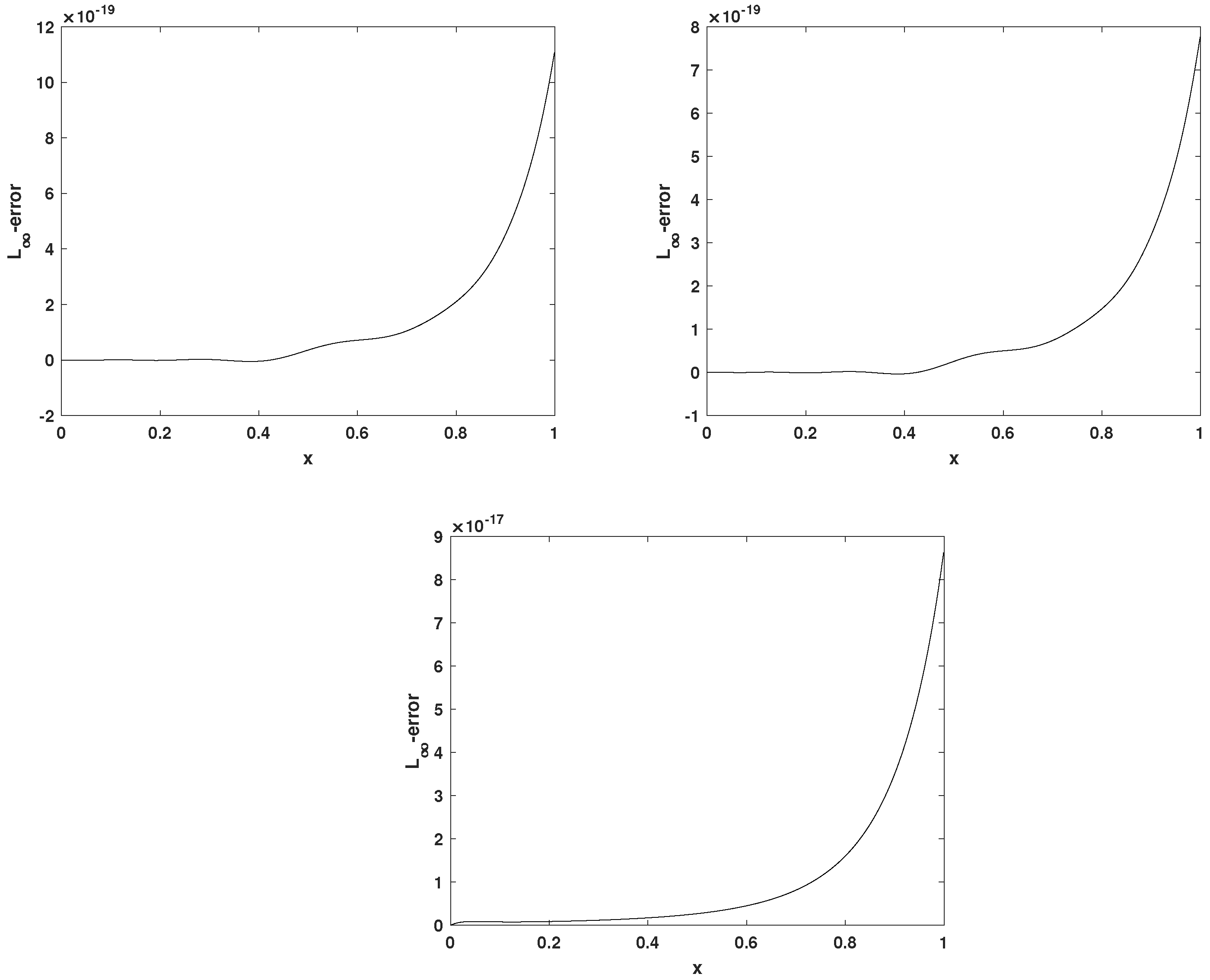
4. Numerical Simulations and Results

To demonstrate the performance of the present method, some examples are provided in this section. To illustrate the results and make a global view of the present method and its efficiency, sometimes, the absolute errors

$$e_N=|u\left(x\right)-u_N\left(x\right)|,$$

and $L_2$ error

$$L^2-error={\left({\int }_0^1{|u\left(x\right)-u_N\left(x\right)|}^2\right)}^{1/2},$$

are reported in Tables or plotted in Figures.

All examples are carried out with the combined use of Maple and Matlab software (version 2022) with an Intel(R) Core(TM) i7-7700k CPU 4.20 GHz (RAM 32 GB).

Example 1.

To contrast the suggested approach with the one described in [1], we consider the following WSIDE:

$${}^C{\mathcal{D}}_0^{1/3}u\left(x\right)=-\frac{32}{35}{x}^{1/2}u\left(x\right)+{\int }_0^x{(x-t)}^{-1/2}u\left(t\right)dt+f\left(x\right),x\in [0,1],$$

with $u\left(0\right)=0$, and

$$f\left(x\right)=\frac{6x^{8/3}}{\mathrm{\Gamma }(11/3)}+\left(32/35-\frac{\mathrm{\Gamma }(1/2)\mathrm{\Gamma }(7/3)}{\mathrm{\Gamma }(17/6)}\right)x^{11/6}+\mathrm{\Gamma }(7/3)x.$$

It is worth mentioning that $u\left(x\right)=x^3+x^{4/3}$ is the exact solution for this example.

To demonstrate the effect of choosing the collocation points, we report

Table 1. The absolute error at different points, taking $\nu =2/3$, for Example 1.

	$\mathit{r}\setminus \mathit{x}$	$0.1$	$0.3$	$0.5$	$0.7$	$0.9$	CPU Time
Chebyshev nodes	5	$8.26\times {10}^{-4}$	$1.30\times {10}^{-3}$	$4.40\times {10}^{-3}$	$4.56\times {10}^{-3}$	$3.33\times {10}^{-3}$	$0.438$
	9	$3.72\times {10}^{-5}$	$5.33\times {10}^{-6}$	$1.41\times {10}^{-4}$	$1.18\times {10}^{-4}$	$8.99\times {10}^{-5}$	$1.125$
Legendre nodes	5	$9.00\times {10}^{-4}$	$7.99\times {10}^{-4}$	$3.29\times {10}^{-3}$	$3.09\times {10}^{-3}$	$2.15\times {10}^{-3}$	$0.485$
	9	$1.88\times {10}^{-5}$	$1.07\times {10}^{-5}$	$8.10\times {10}^{-5}$	$6.76\times {10}^{-5}$	$4.52\times {10}^{-5}$	$1.125$
Uniform meshes	5	$2.07\times {10}^{-2}$	$1.91\times {10}^{-2}$	$1.58\times {10}^{-2}$	$1.55\times {10}^{-2}$	$2.15\times {10}^{-2}$	$0.094$
	9	$1.76\times {10}^{-4}$	$1.25\times {10}^{-4}$	$1.25\times {10}^{-4}$	$1.43\times {10}^{-4}$	$1.58\times {10}^{-4}$	$0.531$

. In

Table 2. A comparison between the presented method and TCM [1] for Example 1.

	Proposed Method		TCM [1]
	$\mathit{r}=\mathbf{5}$	$\mathit{r}=\mathbf{9}$	$\mathit{h}=\mathbf{1}/\mathbf{5}$	$\mathit{h}=\mathbf{1}/\mathbf{10}$
Error	$3.51\times {10}^{-3}$	$8.76\times {10}^{-5}$	$2.08\times {10}^{-2}$	$5.18\times {10}^{-3}$

, we compare the proposed method using Legendre nodes and the trapezoidal collocation method (TCM) [1]. We demonstrate the effect of increasing parameter r with different collocation points in Figure 1. According to the results, reported in the tables and in Figure 1, using the Legendre nodes gives better accuracy for this example. Also, compared to the trapezoidal collocation method, the presented method has better results.

Example 2.

The following example focuses on the equation

$${}^C{\mathcal{D}}_0^{\beta }u\left(x\right)=\frac{1}{2}{\int }_0^x{(x-t)}^{-1/2}u\left(t\right)dt+f\left(x\right),x\in [0,1],$$

with $u\left(0\right)=0$, and

$$f\left(x\right)=2x+3x^2-\frac{1/2x^{5/2}\mathrm{\Gamma }\left(3\right)}{\mathrm{\Gamma }(7/2)}-\frac{1/2x^{7/2}\mathrm{\Gamma }\left(4\right)}{\mathrm{\Gamma }(9/2)}.$$

Note that $u\left(x\right)=x^3+x^2$ is the exact solution of this equation for $\beta =1$.

Considering that by choosing all three types of collocation points, the exact solution is obtained by choosing $r=4$, so the results are reported only by choosing Chebyshev nodes.

Recall that CFD of a function u tends to integer derivative as $\beta \to n$, viz.

$$\begin{array}{c}\underset{\beta \to n}{lim}{}^c{D}^{\beta }u\left(x\right)=u^{\left(n\right)}\left(x\right),\hfill \\ \\ \underset{\beta \to n-1}{lim}{}^c{D}^{\beta }u\left(x\right)=u^{(n-1)}\left(x\right)-u^{(n-1)}\left(0\right).\hfill \end{array}$$

To demonstrate this effect, our results illustrated in Figure 2, obviously, demonstrate it. We can see that when $\beta \to n$, the approximate solution with increasing β tends to the results for n. To show the efficiency and accuracy of the method, we reported the absolute value error in Figure 3 for $\beta =1$, taking $r=4$, $J=1$ and $\nu =1$.

Example 3.

For the third one, we consider the equation

$${}^C{\mathcal{D}}_0^{1/2}u\left(x\right)=e^{x}u\left(x\right)+{\int }_0^x{(x-t)}^{-1/2}u\left(t\right)dt+f\left(x\right),x\in [0,1],$$

with $u\left(0\right)=0$, and

$$f\left(x\right)=\sqrt{2}\left(cos\left(x\right)-sin\left(x\right)\right)\mathrm{C}\left(\frac{\sqrt{2x}}{\sqrt{\pi }}\right)+\sqrt{2}\left(sin\left(x\right)+cos\left(x\right)\right)\mathrm{S}\left(\frac{\sqrt{2x}}{\sqrt{\pi }}\right)-{\mathrm{e}}^{x}sin\left(x\right),$$

in which $S\left(x\right)$ and $C\left(x\right)$ are the Fresnel integrals. The exact solution is considered for this example to be $u\left(x\right)=sin\left(x\right)$.

Table 3. The absolute error at different points, taking $\nu =1$, for Example 3.

	$\mathit{r}\setminus \mathit{x}$	$0.1$	$0.3$	$0.5$	$0.7$	$0.9$	CPU Time
Chebyshev nodes	5	$4.44\times {10}^{-6}$	$8.12\times {10}^{-7}$	$2.82\times {10}^{-5}$	$4.34\times {10}^{-5}$	$2.10\times {10}^{-4}$	$0.360$
	9	$2.80\times {10}^{-12}$	$3.68\times {10}^{-11}$	$2.80\times {10}^{-10}$	$9.56\times {10}^{-10}$	$3.91\times {10}^{-9}$	$0.937$
Legendre nodes	5	$2.08\times {10}^{-6}$	$3.41\times {10}^{-6}$	$2.37\times {10}^{-5}$	$4.94\times {10}^{-5}$	$2.37\times {10}^{-4}$	$0.359$
	9	$2.59\times {10}^{-12}$	$2.83\times {10}^{-11}$	$2.14\times {10}^{-10}$	$7.24\times {10}^{-10}$	$2.97\times {10}^{-9}$	$0.406$
Uniform meshes	5	$1.39\times {10}^{-5}$	$1.58\times {10}^{-5}$	$3.99\times {10}^{-5}$	$1.18\times {10}^{-4}$	$5.00\times {10}^{-4}$	$0.406$
	9	$4.35\times {10}^{-10}$	$6.30\times {10}^{-10}$	$1.44\times {10}^{-9}$	$4.37\times {10}^{-9}$	$1.88\times {10}^{-8}$	$0.500$

is tabulated to demonstrate the effect of picking the collocation points. We illustrate the effect of increasing parameter r with different collocation points in Figure 4. We have also presented Figure 5 to show the accuracy of the method with different choices of collocation points.

Example 4.

Consider the following WSIDE

$${}^C{\mathcal{D}}_0^{1/2}u\left(x\right)=\frac{1}{2}u\left(x\right)+{\int }_0^x{(x-t)}^{-1/2}u\left(t\right)dt+f\left(x\right),x\in [0,1],$$

with $u\left(0\right)=0$, and

$$f\left(x\right)=\frac{\sqrt{\pi }}{2}-\frac{\pi x}{2}-\frac{\sqrt{x}}{2}.$$

The exact solution is considered for this example to be $u\left(x\right)=\sqrt{x}$.

To illustrate the efficiency of the presented method for a non-smooth solution near the origin, the absolute error of approximation is plotted in Figure 6. As we observe, the accuracy of the approximate solution near the origin is also good. To demonstrate the effect of choosing the collocation points, we report

Table 4. The absolute error at different points, taking $\nu =1/8$, for Example 4.

	$\mathit{r}\setminus \mathit{x}$	$0.1$	$0.3$	$0.5$	$0.7$	$0.9$	CPU Time
Chebyshev nodes	12	$1.67\times {10}^{-4}$	$2.34\times {10}^{-4}$	$3.67\times {10}^{-4}$	$5.94\times {10}^{-4}$	$1.00\times {10}^{-3}$	$8.046$
	20	$2.87\times {10}^{-5}$	$3.81\times {10}^{-5}$	$6.06\times {10}^{-5}$	$9.98\times {10}^{-5}$	$1.66\times {10}^{-4}$	$75.250$
Legendre nodes	12	$2.20\times {10}^{-4}$	$3.02\times {10}^{-4}$	$4.77\times {10}^{-4}$	$7.74\times {10}^{-4}$	$1.30\times {10}^{-3}$	$8.203$
	20	$3.22\times {10}^{-5}$	$4.28\times {10}^{-5}$	$6.81\times {10}^{-5}$	$1.12\times {10}^{-4}$	$1.86\times {10}^{-4}$	$75.265$
Uniform meshes	12	$2.04\times {10}^{-4}$	$2.81\times {10}^{-4}$	$4.44\times {10}^{-4}$	$7.20\times {10}^{-4}$	$1.21\times {10}^{-3}$	$8.172$
	20	$4.79\times {10}^{-5}$	$6.36\times {10}^{-5}$	$1.01\times {10}^{-4}$	$1.67\times {10}^{-4}$	$2.77\times {10}^{-4}$	$83.828$

.

5. Conclusions

The main objective of this work is to solve the WSIDE using the collocation method and Müntz–Legendre wavelet. We use the collocation approach to solve the problem after reducing the desired equation to a weakly singular Volterra integral equation. To accomplish this, the Volterra equation is reduced to a system of nonlinear algebraic equations using the fractional integration operational matrix. We can determine the unknown coefficients U after solving this system. The collocation points in this study are uniformly spaced meshes or the roots of shifted Legendre and Chebyshev polynomials. The numerical simulations illustrate the method’s effectiveness and correctness. The proposed method offers superior outcomes compared to some existing methods. The error bound for the desired equation based on the presented method is investigated.

In the future, we plan to extend our numerical approaches for solving generalized fractional models, including the generalized time-space fractional diffusion equations with variable coefficients [44] and time-fractional diffusion equations with a time-invariant type variable order [45], etc.

References

1. Zhao, J.; Xiao, J.; Ford, N.J. Collocation methods for fractional integro-differential equations with weakly singular kernels. Numer. Algorithms 2014, 65, 723–743. [Google Scholar] [CrossRef]
2. Angstmann, C.N.; Henry, B.I.; McGann, A.V. A fractional order recovery SIR model from a stochastic process. Bull. Math. Biol. 2016, 78, 468–499. [Google Scholar] [CrossRef] [PubMed]
3. Eslahchi, M.R.; Dehghan, M.; Parvizi, M. Application of the collocation method for solving nonlinear fractional integro-differential equations. J. Comput. Appl. Math. 2014, 257, 105–128. [Google Scholar] [CrossRef]
4. Aminikhah, H. A new analytical method for solving systems of linear integro-differential equations. J. King Saud Univ. Sci. 2011, 23, 349–353. [Google Scholar] [CrossRef]
5. Arikoglu, A.; Ozkol, I. Solution of fractional integro-differential equations by using fractional differential transform method. Chaos Solitons Fractals 2009, 40, 521–529. [Google Scholar] [CrossRef]
6. Momani, S.; Noor, M.A. Numerical methods for fourth order fractional integro-differential equations. Appl. Math. Comput. 2006, 182, 754–760. [Google Scholar] [CrossRef]
7. Momani, S.; Qaralleh, A. An Efficient Method for Solving Systems of Fractional Integro-Differential Equations. Comput. Math. Appl. 2006, 52, 459–470. [Google Scholar] [CrossRef]
8. Rawashdeh, E.A. Numerical solution of fractional integro-differential equations by collocation method. Appl. Math. Comput. 2006, 176, 1–6. [Google Scholar] [CrossRef]
9. Chow, T.S. Fractional dynamics of interfaces between soft-nanoparticles and rough substrates. Phys. Lett. A 2005, 342, 148–155. [Google Scholar] [CrossRef]
10. Mandelbrot, B. Some noises with 1/f spectrum, a bridge between direct current and white noise. IEEE Trans. Inform. Theory 1967, 13, 289–298. [Google Scholar] [CrossRef]
11. Magin, R.L. Fractional Calculus in Bioengineering, Illustrated ed.; Begell House: Danbury, CT, USA, 2006. [Google Scholar]
12. He, J.H. Some applications of nonlinear fractional differential equations and their approximations. Bull. Sci. Technol. 1999, 15, 86–90. [Google Scholar]
13. Rossikhin, Y.A.; Shitikova, M.V. Applications of fractional calculus to dynamic problems of linear and nonlinear hereditary mechanics of solids. Appl. Mech. Rev. 1997, 50, 15–67. [Google Scholar] [CrossRef]
14. He, J.H. Nonlinear oscillation with fractional derivative and its applications. In Proceedings of the International Conference on Vibrating Engineering’98, Dalian, China, 25–28 May 1998; pp. 288–291. [Google Scholar]
15. Metzler, R.; Klafter, J. The restaurant at the end of the random walk: Recent developments in the description of anomalous transport by fractional dynamics. J. Phys. A 2004, 37, 161–208. [Google Scholar] [CrossRef]
16. Mainardi, F. Fractional calculus: Some basic problems in continuum and statistical mechanics. In Fractals and Fractional Calculus in Continuum Mechanics; Carpinteri, A., Mainardi, F., Eds.; Springer: New York, NY, USA, 1997. [Google Scholar]
17. Baillie, R.T. Long memory processes and fractional integration in econometrics. J. Econom. 1996, 73, 5–59. [Google Scholar] [CrossRef]
18. Alquran, M.; Jaradat, H.M.; Syam, M.I. Analytical solution of the time-fractional Phi-4 equation by using modified residual power series method. Nonlinear Dynam. 2017, 90, 2525–2529. [Google Scholar] [CrossRef]
19. El-Ajou, A.; Arqub, O.A.; Al Zhour, Z.; Momani, S. New results on fractional power series: Theories and applications. Entropy 2013, 15, 5305–5323. [Google Scholar] [CrossRef]
20. Qazza, A.; Saadeh, R.; Salah, E. Solving fractional partial differential equations via a new scheme. AIMS Math. 2022, 8, 5318–5337. [Google Scholar] [CrossRef]
21. Zhang, Y. A finite difference method for fractional partial differential equation. Appl. Math. Comput. 2009, 215, 524–529. [Google Scholar] [CrossRef]
22. Bonyadi, S.; Mahmoudi, Y.; Lakestani, M.; Jahangiri rad, M. Numerical solution of space-time fractional PDEs with variable coefficients using shifted Jacobi collocation method. Comput. Methods Differ. Equ. 2023, 11, 81–94. [Google Scholar]
23. Shahriari, M.; Saray, B.N.; Mohammadalipour, B.; Saeidian, S. Pseudospectral method for solving the fractional one-dimensional Dirac operator using Chebyshev cardinal functions. Phys. Scr. 2023, 98, 055205. [Google Scholar] [CrossRef]
24. Yang, X.; Wu, L.; Zhang, H. A space-time spectral order sinc-collocation method for the fourth-order nonlocal heat model arising in viscoelasticity. Appl. Math. Comput. 2023, 457, 128192. [Google Scholar] [CrossRef]
25. Zhang, H.; Yang, X.; Tang, Q.; Xu, D. A robust error analysis of the OSC method for a multi-term fourth-order sub-diffusion equation. Comput. Math. Appl. 2022, 109, 180–190. [Google Scholar] [CrossRef]
26. Asadzadeh, M.; Saray, B.N. On a multiwavelet spectral element method for integral equation of a generalized Cauchy problem. BIT 2022, 62, 383–1416. [Google Scholar] [CrossRef]
27. Li, C.; Li, Z.; Wang, Z. Mathematical analysis and the local discontinuous Galerkin method for Caputo–Hadamard fractional partial differential equation. J. Sci. Comput. 2020, 85, 41. [Google Scholar] [CrossRef]
28. Mao, Z.; Shen, J. Efficient spectral–Galerkin methods for fractional partial differential equations with variable coefficients. J. Comput. Phys. 2016, 307, 243–261. [Google Scholar] [CrossRef]
29. Ford, N.J.; Xiao, J.; Yan, Y. A finite element method for time fractional partial differential equations. Fract. Calc. Appl. Anal. 2011, 14, 454–474. [Google Scholar] [CrossRef]
30. Shah, N.A.; El-Zahar, E.R.; Akgül, A.; Khan, A.; Kafle, J. Analysis of Fractional-Order Regularized Long-Wave Models via a Novel Transform. J. Funct. Spaces 2022, 2022, 2754507. [Google Scholar] [CrossRef]
31. Alpert, B.; Beylkin, G.; Coifman, R.R.; Rokhlin, V. Wavelet-like bases for the fast solution of second-kind integral equations. SIAM J. Sci. Stat. Comput. 1993, 14, 159–184. [Google Scholar] [CrossRef]
32. Heller, V.; Strang, G.; Topiwala, P.N.; Heil, C. The application of multiwavelet filterbanks to image processing. IEEE Trans. Image Process. 1999, 8, 548–563. [Google Scholar]
33. Saray, B.N. Abel’s integral operator: Sparse representation based on multiwavelets. BIT Numer. Math. 2021, 61, 587–606. [Google Scholar] [CrossRef]
34. Saray, B.N. An effcient algorithm for solving Volterra integro-differential equations based on Alpert’s multi-wavelets Galerkin method. J. Comput. Appl. Math. 2019, 348, 453–465. [Google Scholar] [CrossRef]
35. Saray, B.N. Sparse multiscale representation of Galerkin method for solving linear-mixed Volterra-Fredholm integral equations. Math. Method Appl. Sci. 2020, 43, 2601–2614. [Google Scholar] [CrossRef]
36. Rahimkhani, P.; Ordokhani, Y.; Babolian, E. Müntz-Legendre wavelet operational matrix of fractional-order integration and its applications for solving the fractional pantograph differential equations. Numer. Algorithms 2018, 77, 1283–1305. [Google Scholar] [CrossRef]
37. Jebreen, H.B.; Tchier, F. A New Scheme for Solving Multiorder Fractional Differential Equations Based on Müntz–Legendre Wavelets. Complexity 2021, 2021, 9915551. [Google Scholar] [CrossRef]
38. Rahimkhani, P.; Ordokhani, Y. Numerical solution a class of 2D fractional optimal control problems by using 2D Müntz-Legendre wavelets. Optim. Contr. Appl. Met. 2018, 39, 1916–1934. [Google Scholar] [CrossRef]
39. Almira, J.M. Müntz type theorems. I Surv. Approx. Theory 2007, 3, 152–194. [Google Scholar]
40. Müntz, C.H. Über den Approximationssatz von Weierstrass. In Mathematische Abhandlungen Hermann Amandus Schwarz; Springer: Berlin/Heidelberg, Germany, 1914; pp. 303–312. [Google Scholar]
41. Shen, J.; Wang, Y. Müntz-Galerkin methods and applicationa to mixed dirichlet-neumann boundary value problems. Siam J. Sci. Comput. 2016, 38, 2357–2381. [Google Scholar] [CrossRef]
42. Borwein, P.; Erdélyi, T.; Zhang, J. Müntz systems and orthogonal Müntz–Legendre polynomials. Trans. Am. Math. Soc. 1994, 342, 523–542. [Google Scholar]
43. Kilbas, A.; Srivastava, H.M.; Trujillo, J.J. Theory and Applications of Fractional Differential Equations, 24; Elsevier B.V.: Amsterdam, The Netherlands, 2006. [Google Scholar]
44. Gu, X.M.; Huang, T.Z.; Zhao, Y.L.; Lyu, P.; Carpentieri, B. A fast implicit difference scheme for solving the generalized time–space fractional diffusion equations with variable coefficients. Numer. Methods Partial Differ. Equ. 2021, 37, 1136–1162. [Google Scholar] [CrossRef]
45. Gu, X.M.; Sun, H.W.; Zhao, Y.L.; Zheng, X. An implicit difference scheme for time-fractional diffusion equations with a time-invariant type variable order. Appl. Math. Lett. 2021, 120, 107270. [Google Scholar] [CrossRef]
Figure 1. The influence of the multiplicity parameter r on L 2 -errors for Example 1.
Fractalfract 07 00763 g001
Figure 2. Approximate solutions associated with different values of β , when ν = 1 , r = 4 and J = 1 , for Example 2.
Fractalfract 07 00763 g002
Figure 3. Plot of absolute error for Example 2.
Fractalfract 07 00763 g003
Figure 4. The effect of multiplicity parameter r on L 2 -errors for Example 3.
Fractalfract 07 00763 g004
Figure 5. The absolute errors using Chebyshev nodes (top left), Legendre nodes (top right) and Uniform meshes for Example 3, taking r = 15 and ν = 1 .
Fractalfract 07 00763 g005
Figure 6. The absolute error using the Chebyshev nodes, taking ν = 1 / 8 , r = 20 , for Example 4.
Fractalfract 07 00763 g006