Cryptocurrency Price Prediction Using Frequency Decomposition and Deep Learning

Abstract

Given the substantial volatility and non-stationarity of cryptocurrency prices, forecasting them has become a complex task within the realm of financial time series analysis. This study introduces an innovative hybrid prediction model, VMD-AGRU-RESVMD-LSTM, which amalgamates the disintegration–integration framework with deep learning techniques for accurate cryptocurrency price prediction. The process begins by decomposing the cryptocurrency price series into a finite number of subseries, each characterized by relatively simple volatility patterns, using the variational mode decomposition (VMD) method. Next, the gated recurrent unit (GRU) neural network, in combination with an attention mechanism, predicts each modal component’s sequence separately. Additionally, the residual sequence, obtained after decomposition, undergoes further decomposition. The resultant residual sequence components serve as input to an attentive GRU (AGRU) network, which predicts the residual sequence’s future values. Ultimately, the long short-term memory (LSTM) neural network integrates the predictions of modal components and residuals to yield the final forecasted price. Empirical results obtained for daily Bitcoin and Ethereum data exhibit promising performance metrics. The root mean square error (RMSE) is reported as 50.651 and 2.873, the mean absolute error (MAE) stands at 42.298 and 2.410, and the mean absolute percentage error (MAPE) is recorded at 0.394% and 0.757%, respectively. Notably, the predictive outcomes of the VMD-AGRU-RESVMD-LSTM model surpass those of standalone LSTM and GRU models, as well as other hybrid models, confirming its superior performance in cryptocurrency price forecasting.

1. Introduction

Since its inception in 2009, cryptocurrency has experienced an unprecedentedly high growth rate and market capitalization share over a mere decade, disrupting traditional financial assets and derivatives [1,2], thus emerging as a highly promising investment avenue [3]. By November 2021, the total market capitalization of cryptocurrencies had surged to USD 3 trillion. As the cryptocurrency market has evolved, the urgent need for cryptocurrency price prediction has intensified among investors and research entities due to its substantial returns and prolonged periods of heightened volatility [4,5]. This urgency has made cryptocurrency price prediction a focal point within the field of financial time series forecasting. Accurate forecasts of cryptocurrency prices can furnish investors and research entities with valuable insights, facilitating well-informed decisions, deterring unethical speculation and fraud, and mitigating unwarranted market panic. Therefore, the enhancement of cryptocurrency prediction methodologies, the augmentation of prediction precision, and the mitigation of investment risks for stakeholders will play a pivotal role in fostering the healthy and stable development of the cryptocurrency market.

Traditional statistical and econometric models in linear time series forecasting such as ARIMA, as well as non-linear models such as autoregressive conditional heteroskedasticity (ARCH) and vector autoregressive (VAR), are all rooted in the assumption of stationarity. These methods require non-stationary data to be transformed into stationary data before prediction. Additionally, their handling of non-linear issues is not optimal, leading to inherent limitations when applied to financial time series predictions. Furthermore, these methods struggle to meet the demands for prediction accuracy and efficiency. In this context, the emergence of machine learning and deep learning methods has showcased their advantages in forecasting cryptocurrency prices [6,7].

With the rise of research in the field of artificial intelligence, epitomized by machine learning, an increasing number of machine learning models have been integrated into time series forecasting tasks. Unlike traditional statistical and econometric models, these non-linear and non-parametric models have demonstrated higher predictive accuracy in time series forecasting. Classical machine learning models, such as decision trees, random forests, and support vector machines, often rely on feature engineering, necessitating preprocessing and feature selection. However, for larger-scale financial data, feature selection becomes challenging. Moreover, when dealing with multidimensional financial data, issues such as the curse of dimensionality and overfitting can arise.

As the size of datasets continues to grow, accompanied by remarkable advancements in data storage capacity and computing power, the expansion of computer memory has progressed relatively slower. This has led to the possibility of constructing larger models with a higher number of parameters while striving to enhance memory efficiency. Consequently, numerous deep learning methods have found application in financial time series forecasting. Deep learning does not necessitate the assumption of stationarity, granting it an innate advantage in predicting financial time series. The architecture of deep neural networks contributes to their strong generalization capabilities. Networks such as gated recurrent units (GRU) and long short-term memory (LSTM) utilize their internal structures to extract temporal correlations from time series data. A study showed that the incorporation of recurrent dropout in a GRU model notably enhanced the predictive performance for Bitcoin price compared to baseline models [8]. Hence, in this study, a GRU model is adopted as the foundational predictor within a hybrid model structure.

Despite the commendable performance of deep learning models in time series forecasting, these models still encounter challenges in identifying the importance of input features. Attention mechanisms address this issue by enabling deep learning models to adaptively discern the significance of input features. Therefore, this study employs a combination of a GRU network and an attention mechanism for forecasting.

Compared to traditional financial markets, the cryptocurrency market exhibits an intense speculative nature, contributing to higher volatility and non-stationarity in cryptocurrency price sequences compared to general financial time series. Conventional standalone deep learning models often struggle to achieve outstanding predictive accuracy when forecasting such sequences [9].

Extracting underlying features from the original sequence can further enhance predictive performance for the raw data. By decomposing the original time series into relatively simpler modal components, estimating them separately, and then integrating them to generate the final prediction output, it is possible to achieve enhanced predictive performance. Modal decomposition involves breaking down complex and non-stationary cryptocurrency price sequences characterized by challenging market volatility into a series of relatively simple modal components. This approach facilitates the model’s ability to capture the intrinsic characteristics of the time series. This ensemble model, based on the decomposition–integration framework, demonstrates higher predictive accuracy in financial time series forecasting compared to single models [10]. Hence, we adopt the decomposition–integration framework as the architecture for our hybrid model.

The commonly used empirical mode decomposition (EMD) is a primary method for decomposing non-stationary time series data into intrinsic mode functions (IMFs). EMD decomposition is advantageous in dealing with noisy data by leveraging the time scale characteristics inherent to the data itself. It does not require predefined basis functions, making it particularly effective for processing non-stationary and non-linear data. However, EMD suffers from endpoint effects and mode mixing issues, leading to increased prediction errors. In contrast, the variational mode decomposition (VMD) method can overcome challenges, such as mode mixing, improper envelopes, and boundary instability, that often arise during the decomposition process [11]. Consequently, VMD maintains stability when handling non-linear and non-stationary data. Moreover, sequences obtained through VMD tend to be smoother, making it easier for deep learning models to capture the patterns within these subsequences.

Nonetheless, a drawback of VMD is that it leaves behind a residual component. In current research [12,13], either this residual is treated as an additional mode for prediction, which is challenging due to its complex characteristics, leading to potential errors in the final ensemble prediction, or the residual is directly ignored. In the latter case, disregarding the residual can cause the sum of modal components to deviate from the original sequence, resulting in information loss and ultimately leading to significant prediction errors. To address this issue, this study proposes a residual re-decomposition prediction method that effectively predicts the residual while retaining it, thereby enhancing the accuracy of the final prediction.

In conclusion, this paper introduces a novel hybrid prediction model, namely the VMD-AGRU-RESVMD-LSTM model, designed for single-step forecasting of cryptocurrency prices. The model integrates decomposition ensemble methods, variational mode decomposition (VMD), the gated recurrent unit (GRU) and long short-term memory (LSTM) neural network models, and attention mechanisms. The VMD process decomposes the data, resulting in smoother subsequences that make it easier for the model to capture internal patterns. AGRU subsequence predictors handle various modes, while the attention mechanism effectively identifies significant input features. The RESVMD process re-decomposes residuals before prediction, mitigating errors introduced by residual components. LSTM executes integrated forecasting.

To validate the superiority and robustness of the proposed model, empirical analyses are performed using BTC and ETH datasets. A comprehensive evaluation of predictive performance is conducted using standard evaluation metrics. The robustness of the model is tested through DM tests on datasets with different time spans. Lastly, the predictive results of the VMD-AGRU-RESVMD-LSTM model are subjected to profit and loss back-testing, thus confirming the practical economic significance of the predictive model.

In summary, the contributions of this study are as follows:

• The study introduces a novel hybrid prediction model, VMD-AGRU-RESVMD-LSTM. Empirical results demonstrate the model’s superiority and robustness in both prediction accuracy and simulated profit outcomes.
• In addressing the residuals obtained from VMD decomposition, a novel residual re-decomposition prediction method is proposed in this paper. In contrast to previous approaches to handling residuals, this method mitigates errors, consequently improving predictive accuracy.
• This research presents an attention mechanism that offers a deeper exploration of the internal mechanisms within cryptocurrency price sequences. When combined with the GRU network model, this mechanism effectively mines the inherent features of time series data, resulting in enhanced prediction accuracy.

The remaining sections of the paper are organized as follows. Section 2 provides a comprehensive review of relevant literature in the field. Section 3 explains in detail the methodologies and techniques employed, including variational mode decomposition (VMD), gated recurrent unit (GRU), long short-term memory (LSTM), attention mechanisms, normalization, and the experimental procedure. Section 4 outlines the data used in the study and presents the empirical testing process. It also includes a comparison and analysis of the impacts of various enhancement methods on the experimental outcomes. Section 5 summarizes the entire paper and provides key takeaways from the study.

2. Related Work Literature Review

Commonly used cryptocurrency prediction methods fall into two main categories: econometric and statistical models and machine learning and deep learning models. Most traditional econometric and statistical methods, such as SES, ARIMA, and other models and their variants, are not accurate enough in forecasting highly volatile prices over long periods to capture long-term dependence in the presence of high volatility. Ref. [14] showed that these models have difficulty meeting the volatility and non-stationarity of the cryptocurrency market, and these traditional models are inelastic in predicting different types of cryptocurrencies. Compared with traditional time series models, machine learning and deep learning models have advantages in analyzing nonlinear multivariate data and are robust to noise values. When sufficient data are available, compared with traditional econometric and statistical models, many classical ML models have achieved higher prediction accuracy [15]. With the progress of research on neural networks, today’s deep learning models have achieved higher accuracy in predicting time series. Ref. [8] shows that the recurrent neural network (RNN) using GRU and LSTM is superior to the traditional ML model and that the GRU model with cyclic dropout significantly improves the performance of the Bitcoin price prediction baseline. However, it is difficult for a single model to accurately capture the characteristics of time series, and it is difficult to obtain accurate prediction results in the face of complex and volatile cryptocurrency prices.

The decomposition–integration method shows its superiority in many time series prediction fields, such as carbon prices [16,17], wind power [18,19,20], oil prices [11,21], and air quality [22,23]. The decomposition–integration method has been widely used in the field of financial time series prediction [24,25]. In particular, the research shows that the decomposition–integration method has excellent performance in the prediction of stock prices [10,26] and exchange rates [27]. However, it has an existing application in the field of cryptocurrency price forecasting. The research [28] shows that both cryptocurrencies and traditional financial time series such as stock prices are non-stationary and highly volatile. Ref. [29] shows that, after years of development, cryptocurrencies have become closely related to traditional financial markets such as currencies, stocks, and commodities. At the level of a single time series, cryptocurrencies and foreign exchange markets have almost indistinguishable complex features. The research [30] has shown considerable similarities in the erratic behavior of stocks and cryptocurrencies. According to new research from the International Monetary Fund [31], the correlation between cryptocurrencies and traditional assets such as stocks has increased significantly as market recognition has increased. Cryptocurrencies have become more correlated with the stock market than stocks are with other assets such as gold, investment-grade bonds, and major currencies.

Due to the similar characteristics of cryptocurrency price series and traditional financial time series, this paper attempts to use the decomposition–integration method to predict cryptocurrency price. Empirical mode decomposition (EMD) is the main method used to decompose non-stationary time series data into intrinsic mode functions (IMFs). Ref. [32] used EMD decomposition to decompose financial time series and compared it with wavelet decomposition, proving that the effect of EMD decomposition was better than wavelet decomposition. However, EMD is affected by the endpoint effect and mode mixing, which will lead to an increase in prediction error. In contrast, the VMD method can overcome modal aliasing, improper envelopes, unstable boundaries, and other problems that often occur in the decomposition process, so it still has good stability when dealing with nonlinear and unstable data [11].

Moreover, due to the great success of the self-attention-based Transformer [33] in NLP, attention mechanisms have recently been applied in various fields to solve different problems. The essence of the attention mechanism is to assign global dependencies from input to output. It is a general framework independent of any model and can find the internal relationship between input vectors and output. Research by [34] shows that the attention mechanism has excellent performance in predicting time series. In this study, the attention mechanism and GRU model are combined and applied to the decomposition and integration framework to better mine the features of time series.

This study proposes an emerging hybrid model for cryptocurrency price prediction based on VMD and deep learning methods. Compared with the benchmark model and other hybrid models, our model effectively improves the accuracy of cryptocurrency price prediction.

3. Methodology

3.1. Variational Mode Decomposition

Dragomiretskiy and Zosso put forward the VMD method. By solving variational optimization problems in the frequency domain, the initial complex signals are decomposed into dimensions adaptively, and a series of narrow-band signals with relatively concentrated frequencies are called modal components. Thus, the internal characteristics of the signal can be further explored. The frequencies of the modal components obtained by decomposition are assumed to be concentrated around the respective center frequencies. In the process of VMD decomposition, the following optimization constraint problem is established based on the above component narrow-band conditions:

$$\left\{\begin{array}{c}\underset{\left\{u_k\left\}\right\{{\omega }_k\right\}}{min}\left\{{\displaystyle \sum _K}{∥{\partial }_t\left[\left(\delta \left(t\right)+\frac{j}{\pi t}\right)\ast u_k\left(t\right)\right]e^{-j{\omega }_{k}t}∥}_2^2\right\}\hfill \\ s.t.{\displaystyle \sum _k}{u}_k\left(t\right)=f\hfill \end{array},\right.$$

(1)

in which $f\left(t\right)$ represents the original signal, $\delta \left(t\right)$ represents the unit impulse function, t represents the time, K represents the number of sub-signals, and ∗ represents the convolution operation symbol. To solve this problem, the above equation-constrained optimization problem can be equivalent to an unconstrained optimization problem by introducing the augmented Lagrange function:

$$\begin{array}{c}L\left(\left\{u_k\right\},\left\{{\omega }_k\right\},\lambda \right):=\alpha {\displaystyle \sum _K}{∥{\partial }_t\left[\left(\delta \left(t\right)+\frac{j}{\pi t}\right)\ast u_k\left(t\right)\right]e^{-j{\omega }_{k}t}∥}_2^2\hfill \\ +{∥f\left(t\right)-{\displaystyle \sum _k}{u}_k\left(t\right)∥}_2^2+〈\lambda \left(t\right),f\left(t\right)-{\displaystyle \sum _k}{u}_k\left(t\right)〉\hfill \end{array}.$$

(2)

The alternating direction multiplier direction method (ADMM) can be used to find the optimal solution to the pattern. The basic idea is to fix two variables and update one of them. The expression of variable iteration update is given below:

$$\begin{array}{c}{u}_k^{n+1}=\underset{u_k}{argmin}L\left(\left\{u_{i<k}^{n+1}\right\},\left\{{\omega }_k^n\right\},{\lambda }^n\right);\hfill \\ {\omega }_k^{n+1}=\underset{{\omega }_k}{argmin}L\left(\left\{u_k^n\right\},\left\{{\omega }_{i<k}^{n+1}\right\},{\lambda }^n\right);\hfill \\ {\lambda }^{n+1}={\lambda }^n+\rho \left(f\left(t\right)-{\displaystyle \sum _k}{u}_k^{n+1}\left(t\right)\right).\hfill \end{array}$$

(3)

The convergence condition is:

$$\sum _K^{}{∥{\mu }_{n+1}^k-{\mu }_n^k∥}_2^2/{∥{\mu }_n^k∥}_2^2<\epsilon .$$

(4)

In solving $u_K$, $w_k$, we have:

$$u_k^{n+1}=\frac{f\left(\omega \right)-{\displaystyle \sum _{i\ne k}}{u}_i\left(\omega \right)+\frac{\lambda \left(\omega \right)}{2}}{1+2\alpha {\left(\omega -{\omega }_k\right)}^2},$$

(5)

$${\omega }_k^{n+1}=\frac{{\int }_0^{\infty }\omega \left|u_k\left(\omega \right)\right|d\omega }{{\int }_0^{\infty }\left|u_k\left(\omega \right)\right|d\omega },$$

(6)

where $f\left(w\right),\lambda \left(w\right),u_i\left(w\right),u_{n+1}^k\left(w\right)$ denote the Fourier transform of $f\left(t\right),\lambda \left(t\right),u_i\left(t\right),u_{n+1}^k\left(t\right)$, respectively, and n denotes the number of iterations.

3.2. Long Short-Term Memory

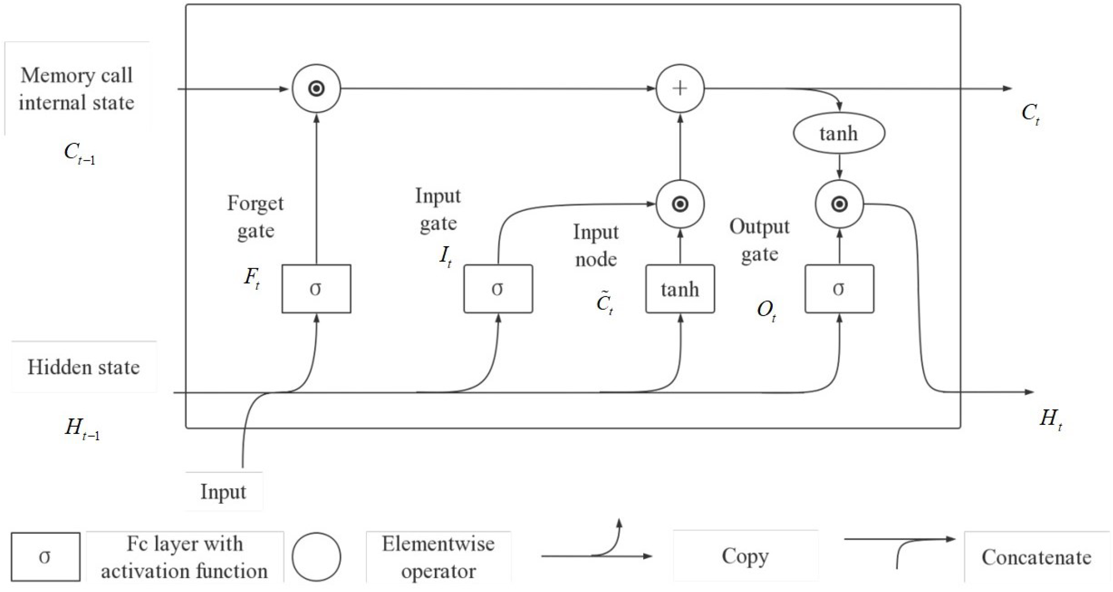
Inspired by computer logic gates, Ref. [35] proposed long short-term memory (LSTM). Based on RNN [36], the gating mechanism and memory unit were introduced to solve the traditional RNN network problem.With the model training, long-term information was difficult to preserve. The short-term information is difficult to update, resulting in information confusion, gradient disappearance, and other problems. The unit characteristics of the LSTM network consist of a memory element (Figure 1), input gate, output gate, and forgetting gate. Memory element $C_t$: Used to record additional information. Input gate $T_t$: Used to determine how much data to enter into memory at the current time t. Output gate $O_t$: used to determine how much data is output by the memory element at the current time t. Forgetting gate $F_t$: Used to determine the degree of retention of the previous memory meta content at the current time t.

$$\begin{array}{c}\hfill \begin{array}{cc}\hfill I_t& =\sigma (X_t{W}_{xi}+H_{t-1}{W}_{hi}+b_i),\hfill \\ \hfill F_t& =\sigma (X_t{W}_{xf}+H_{t-1}{W}_{hf}+b_f),\hfill \\ \hfill O_t& =\sigma (X_t{W}_{xo}+H_{t-1}{W}_{ho}+b_o),\hfill \\ \hfill \widetilde{C_t}& =\tanh (X_t{W}_{xc}+H_{t-1}{W}_{hc}+b_c),\hfill \\ \hfill C_t& =F_t\odot C_{t-1}+I_t\odot {\tilde{C}}_t,\hfill \\ \hfill H_t& =O_t\odot \tanh \left(C_t\right).\hfill \end{array}\end{array}$$

(7)

3.3. Gated Recurrent Unit

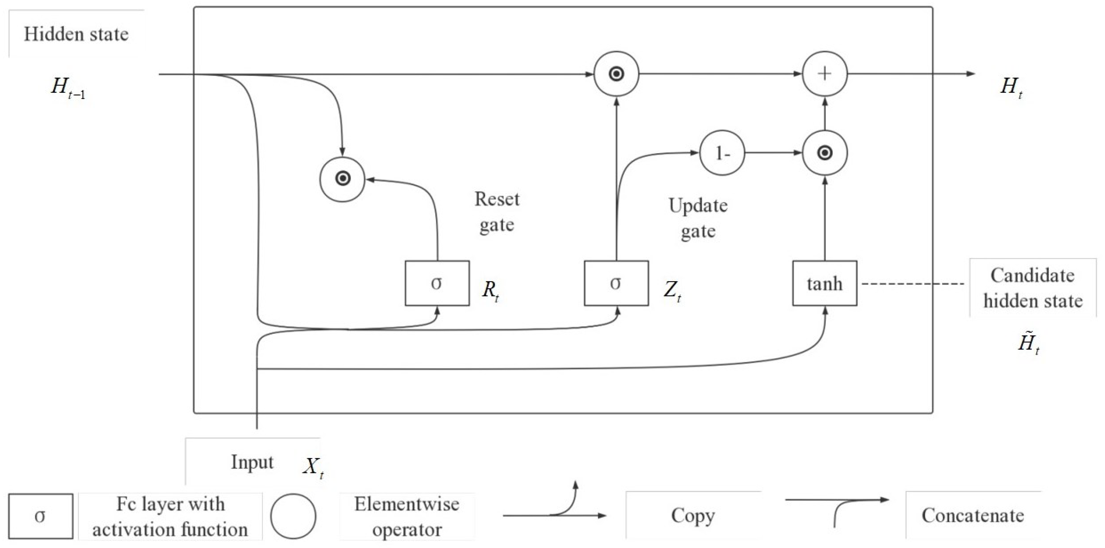
Ref. [36] proposed the gated recurrent unit (GRU), which uses the gating mechanism to control input, memory, and other information to make predictions at the current time step. Similar to the LSTM unit, two gating units are used in GRU, including the reset gate and the update gate. The reset gate defines the degree to which the previous memory is saved to the current time step, and the update gate determines the degree to which the new input information is combined with the previous memory. The unit structure characteristics of GRU (Figure 2) are as follows:

$$\begin{array}{c}\hfill \begin{array}{cc}\hfill R_t& =\sigma (X_t{W}_{xr}+H_{t-1}{W}_{hr}+b_r),\hfill \\ \hfill Z_t& =\sigma (X_t{W}_{xz}+H_{t-1}{W}_{hz}+b_z),\hfill \\ \hfill {\tilde{H}}_t& =\tanh (X_t{W}_{xh}+\left(R_t\odot H_{t-1}\right)W_{hh}+b_h),\hfill \\ \hfill H_t& =Z_t\odot H_{t-1}+(1-Z_t)\odot {\tilde{H}}_t.\hfill \end{array}\end{array}$$

(8)

3.4. Attention Mechanism and AGRU Model

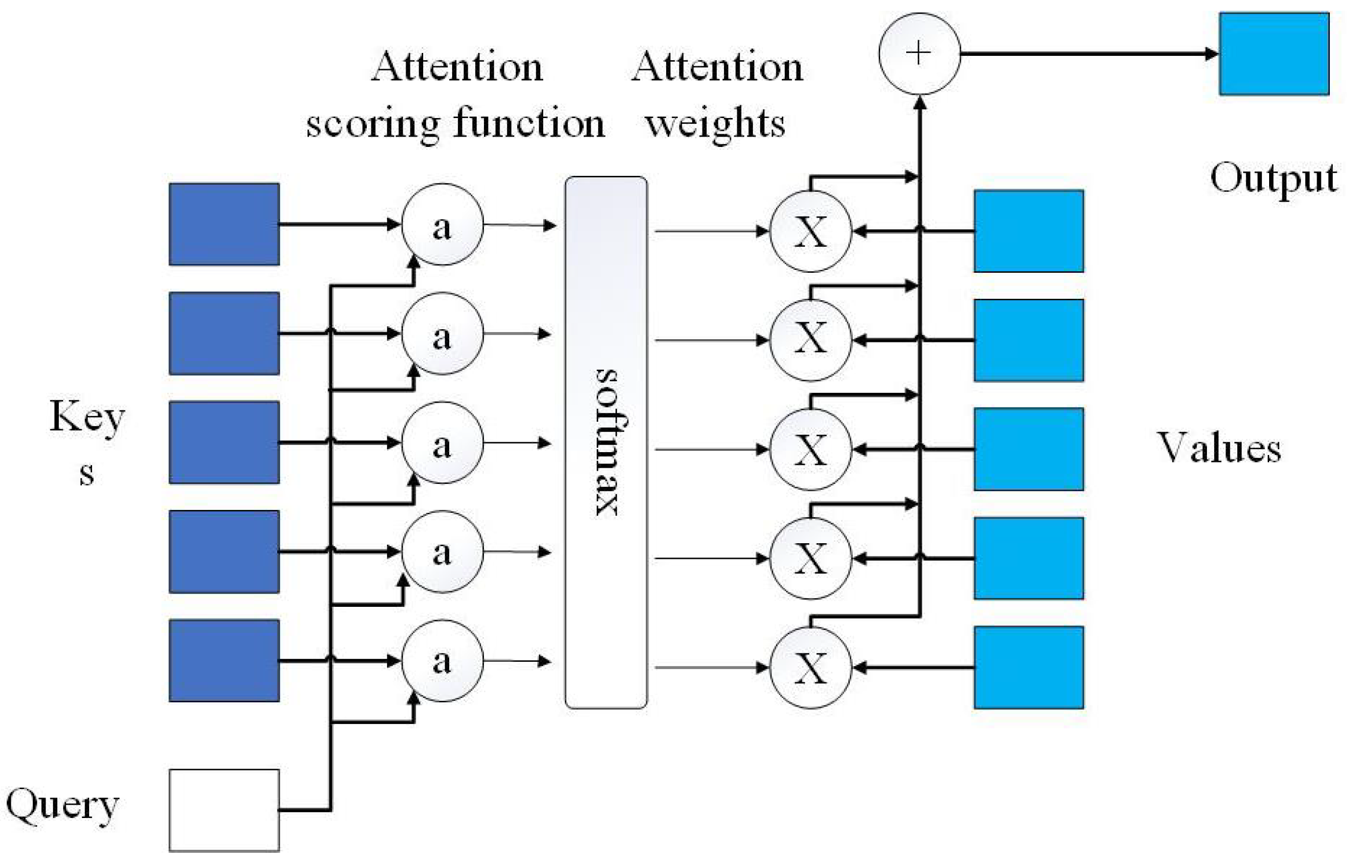
The attention mechanism [33] is a resource allocation mechanism that simulates the human visual mechanism. Its purpose is to allocate more resources to areas with high correlation under limited computing power to obtain more detailed information, which requires more attention and suppression of other useless information. The attention mechanism combines query (autonomous prompt) and key (non-autonomous prompt) through attention convergence to realize the selection tendency of value (sensory input). That is, by combining query and key, a selection tendency of value is realized. Then, for the query in the given target, the correlation of query keys is calculated to obtain the weight coefficient of each key corresponding to the value. Then, the final weighted sum of values is obtaiighted sum of values is obtained. The structural features of the attention mechanism (Figure 3) are as follows:

$$\begin{array}{c}\hfill \begin{array}{c}\hfill f(q,(k_1,v_1),\dots ,(k_m,v_m))=\sum _{i=1}^m\alpha (q,k_i)v_i\in {\mathbb{R}}^v,\\ \hfill \alpha (q,k_i)=\mathrm{softmax}\left(a(q,k_i)\right)=\frac{exp\left(a(q,k_i)\right)}{{\sum }_{j=1}^{m}exp\left(a(q,k_j)\right)}\in \mathbb{R}.\end{array}\end{array}$$

(9)

Instead of the combination of self-attention and GRU units, which is commonly used in serial prediction, we construct an AGRU model that is more in line with the time series mechanism to predict each modal component and improve the prediction accuracy (Figure 4).

3.5. Normalization

Since the target did not pass the Jarque–Bera test, the Min-max method was used to normalize the data in this study. This paper uses the MinMaxScaler function in the Scikit-Learn module to normalize the data.

$$x=\frac{x-x_{min}}{x_{max}-x_{min}}$$

(10)

3.6. Diebold–Mariano Test

The Diebold–Mariano test was used to determine whether the two predictions were significantly different. Let $e_i$ and $r_i$ be the residuals of two predictions and define $d_i$ as the absolute value of the difference between them, i.e., the null hypothesis $(H_0:E\left(d_i\right)=0)$. The DM test assumes that the two series have the same prediction accuracy, and the alternative hypothesis, $(H_0:E\left(D_i\right)\ne 0)$, is that the two series have significantly different prediction accuracy.

$$DM=\sqrt{\frac{\overline{d}}{\widehat{\sigma }}}\to N(0,1)\sim n\to \infty$$

(11)

3.7. Model Evaluation Criteria

In this study, three criteria were used to evaluate prediction performance: root mean square error ($RMSE$)

$$RMSE=\sqrt{\frac{{\sum }_{i=1}^N{(x_i-\widehat{x_i})}^2}{N}},$$

mean absolute error ($MAE$)

$$MAE=\frac{{\sum }_{i=1}^N|x_i-\widehat{x_i}|}{N},$$

and mean absolute percentage error ($MAPE$)

$$MAPE=\sum _{i=1}^N\left|\frac{x_i-\widehat{x_i}}{x_i}\right|.$$

3.8. Framework

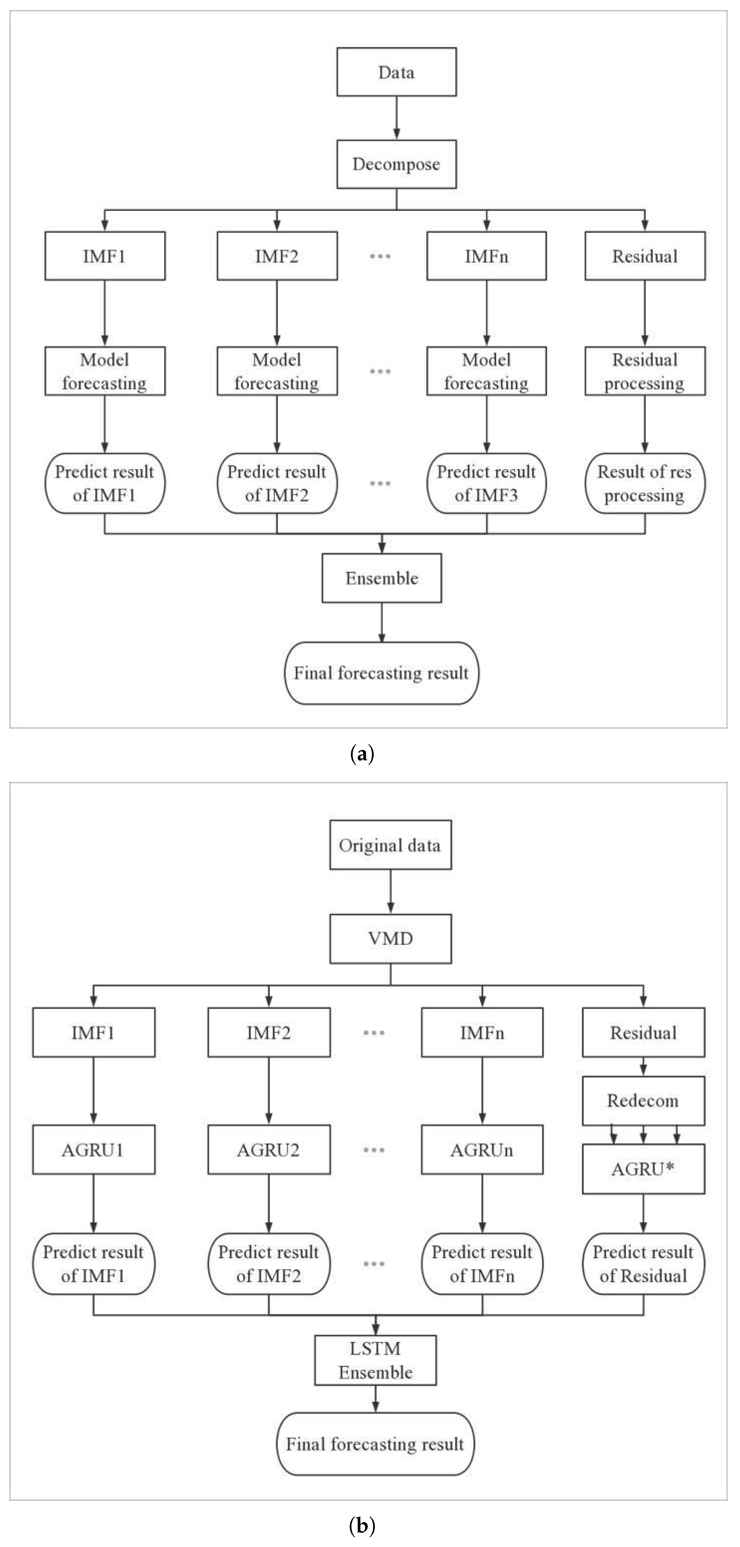
First, a statistical test is done on the target data. The variational mode decomposition is then applied to decompose the cryptocurrency price series into a finite number of subseries with relatively simple volatility patterns. Variational mode decomposition can effectively overcome the shortcomings of end effect and mode mixing in empirical mode decomposition.

Although existing studies have shown that the VMD method can effectively overcome the shortcomings of end effect and mode mixing, they have not systematically tested whether this method is suitable for Bitcoin price prediction. Therefore, when we decompose the Bitcoin price series by VMD, we will use the EMD method for comparison.

Secondly, this study combines a GRU neural network with an attention mechanism to make separate sequence predictions as predictors for each modal component compared with the GRU predictor and the LSTM predictor. At the same time, four different treatments were carried out on the obtained residual sequence: (1) as a modal component processing; (2) discard; (3) further decomposition by EMD and the obtained residual sequence component as the overall input of the AGRU network, to obtain the residual sequence forecast; and (4) further decomposition by VMD and the obtained residual sequence component as the overall input of the predictor, to obtain the residual sequence forecast.

Finally, the LSTM neural network is used to integrate the prediction results of modal components and residuals into the final price compared with the linear method and the GRU neural network (Figure 5). By comparing with some single models and other hybrid models based on empirical mode decomposition and variational mode decomposition, the ability of the model to predict cryptocurrency price is comprehensively verified.

The DM test of the predicted results is used to check whether VMD-AGRU-RESVMD-LSTM is significantly better than the single model and other models based on decomposition integration and deep learning technology.

3.9. Parameter Selection

The number of units of GRU is set as 32, followed by a dropout layer with a dropout probability of 0.2. The number of units of LSTM is set as 32, with a 0.2 dropout layer. The activation function is set as $tanh$. The date-back is set as 30, and the batch is set as 16. Models use the Adam optimizer to calculate the error function. The epoch number is set as 100, and the patience number is set as 10. The shuffle is set as true.

4. Analysis of Experiments

The research in [28] used the daily closing price of cryptocurrencies from 23 July 2017 to 15 July 2020 as the dataset. This research slightly modifies the time span and selects the daily closing price of Bitcoin and Ethereum from 31 July 2017 to 30 September 2020, from which the data from the last 100 days comprise the prediction set.

4.1. Statistical Test of Data and Results of VMD Decomposition

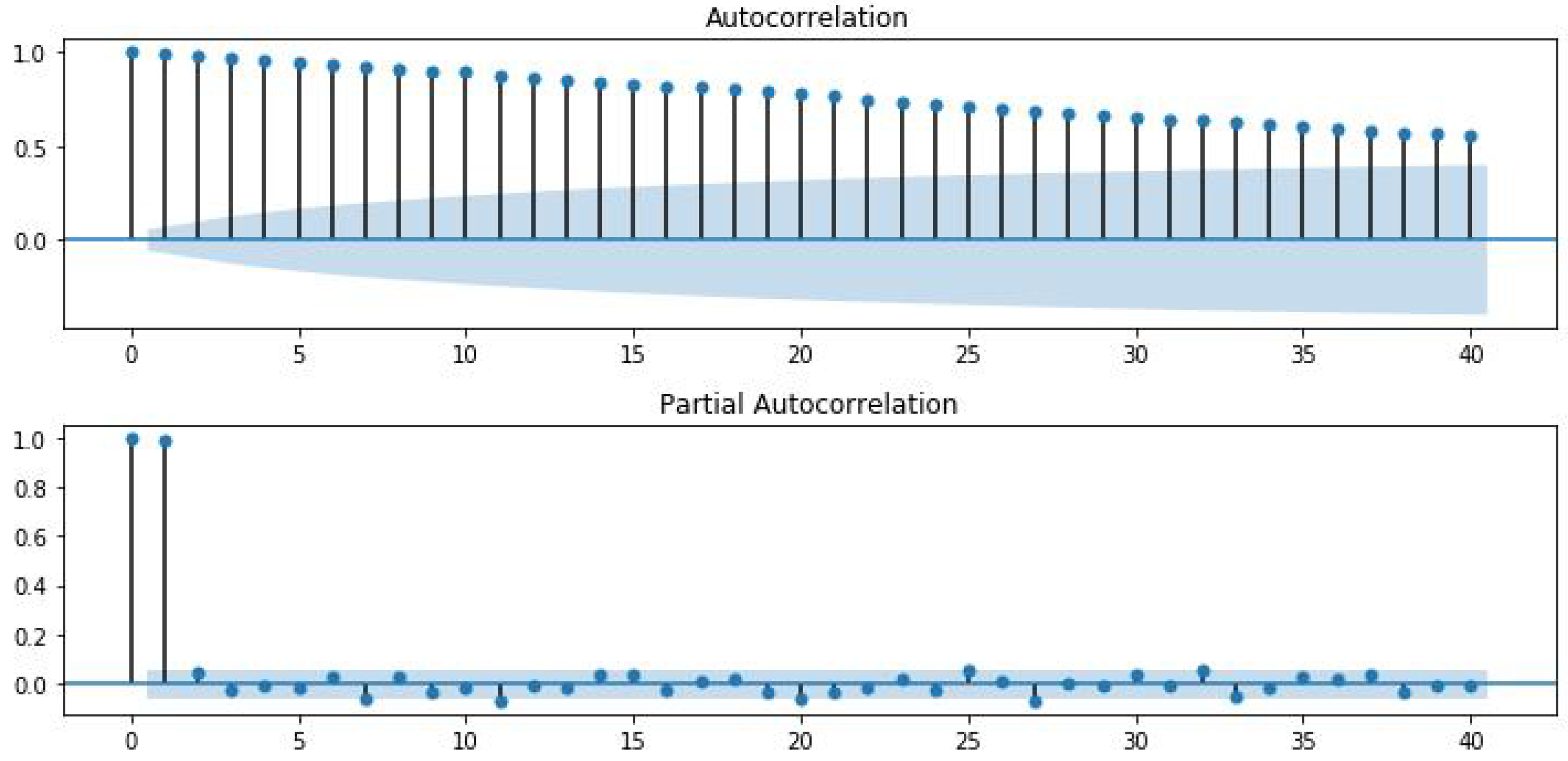
We conducted statistical tests on the Bitcoin price series to explore its stationarity, autocorrelation, and normality (Figure 6). Firstly, the augmented Dickey–Fuller (ADF) test is used to detect the stationarity of the target series. The p value is 0.123, and the ADF value is −2.467, which is greater than the critical value of −2.863 at the 5% significance level, indicating that the target series is non-stationary. Secondly, the Ljung–Box test was used to detect the autocorrelation of the target series, and the p value lag obtained from any lag was 0.00, less than 0.05, which rejected the null hypothesis, indicating that the target series had strong autocorrelation. Furthermore, the Jarque–Bera test was used to test the normality of the target sequence, and the p value of 0.00 was less than 0.05, the skewness was 0.417, and the kurtosis was 3.49. The null hypothesis was rejected, and the target sequence did not follow a normal distribution. Finally, the autocorrelation function (ACF) and partial autocorrelation function (PACF) of the objective function are given, as shown in the figure below, with ACF trailing and PACF at the second-order stage, indicating the autocorrelation of the objective sequence.

We conducted statistical tests on the Ethereum price series to explore its stationarity, autocorrelation, and normality (Figure 7). Firstly, the augmented Dickey–Fuller (ADF) test is used to detect the stationarity of the target sequence. The p value is 0.184, and the ADF value is −2.261, which is greater than the critical value of −2.864 at the 5% significance level, indicating that the target sequence is non-stationary. Secondly, the Ljung–Box test was used to detect the autocorrelation of the target series, and the p value lag obtained from any lag was 0.00, less than 0.05, which rejected the null hypothesis, indicating that the target series had strong autocorrelation. Furthermore, the Jarque–Bera test was used to test the normality of the target sequence, and the p value of 0.00 was less than 0.05, the skewness was 1.937, and the kurtosis was 6.847. The null hypothesis was rejected, and the target sequence did not follow a normal distribution. Finally, the autocorrelation function (ACF) and partial autocorrelation function (PACF) of the objective function are given, as shown in the figure below, with ACF trailing and PACF at the second-order stage, indicating the autocorrelation of the objective sequence.

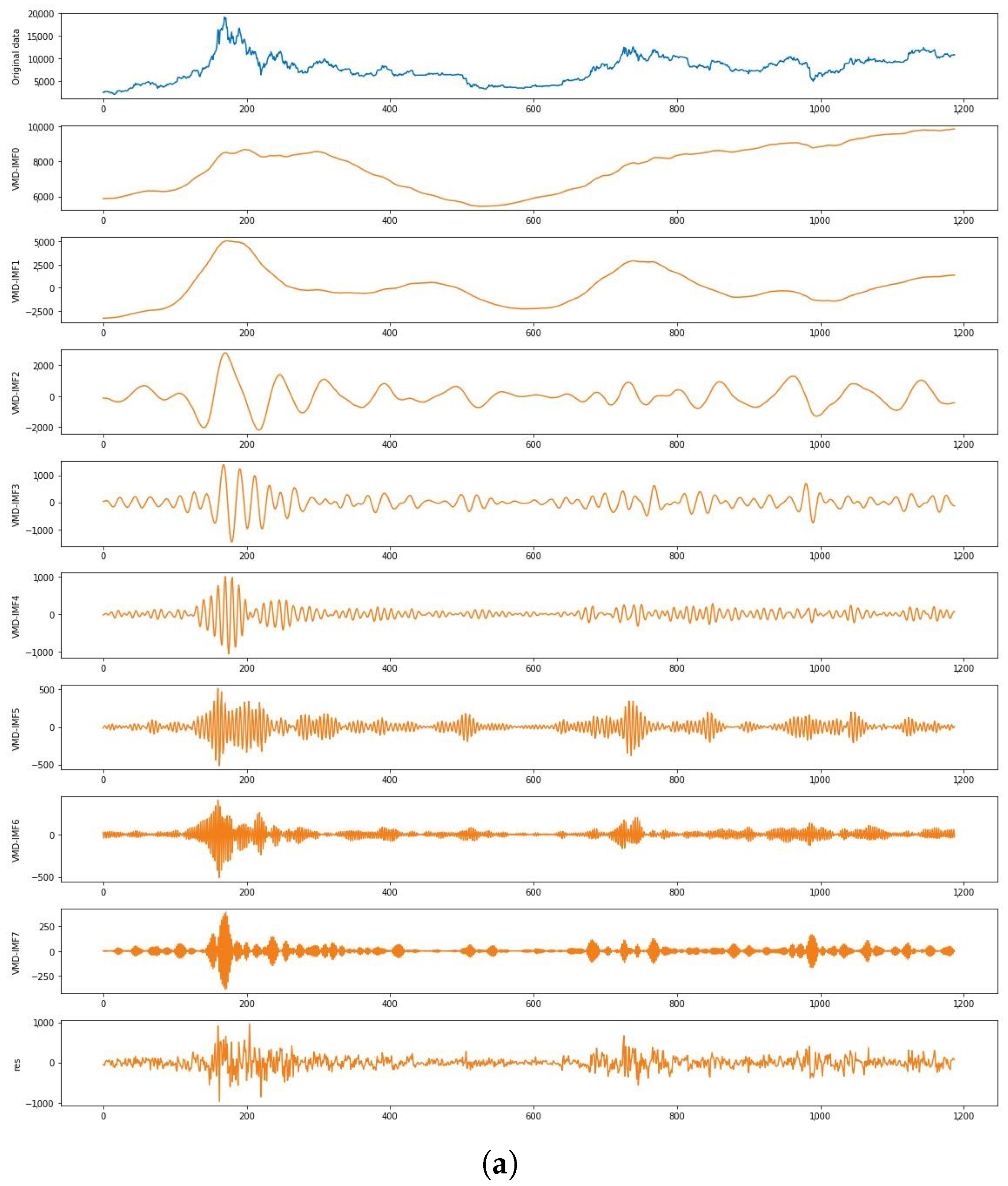
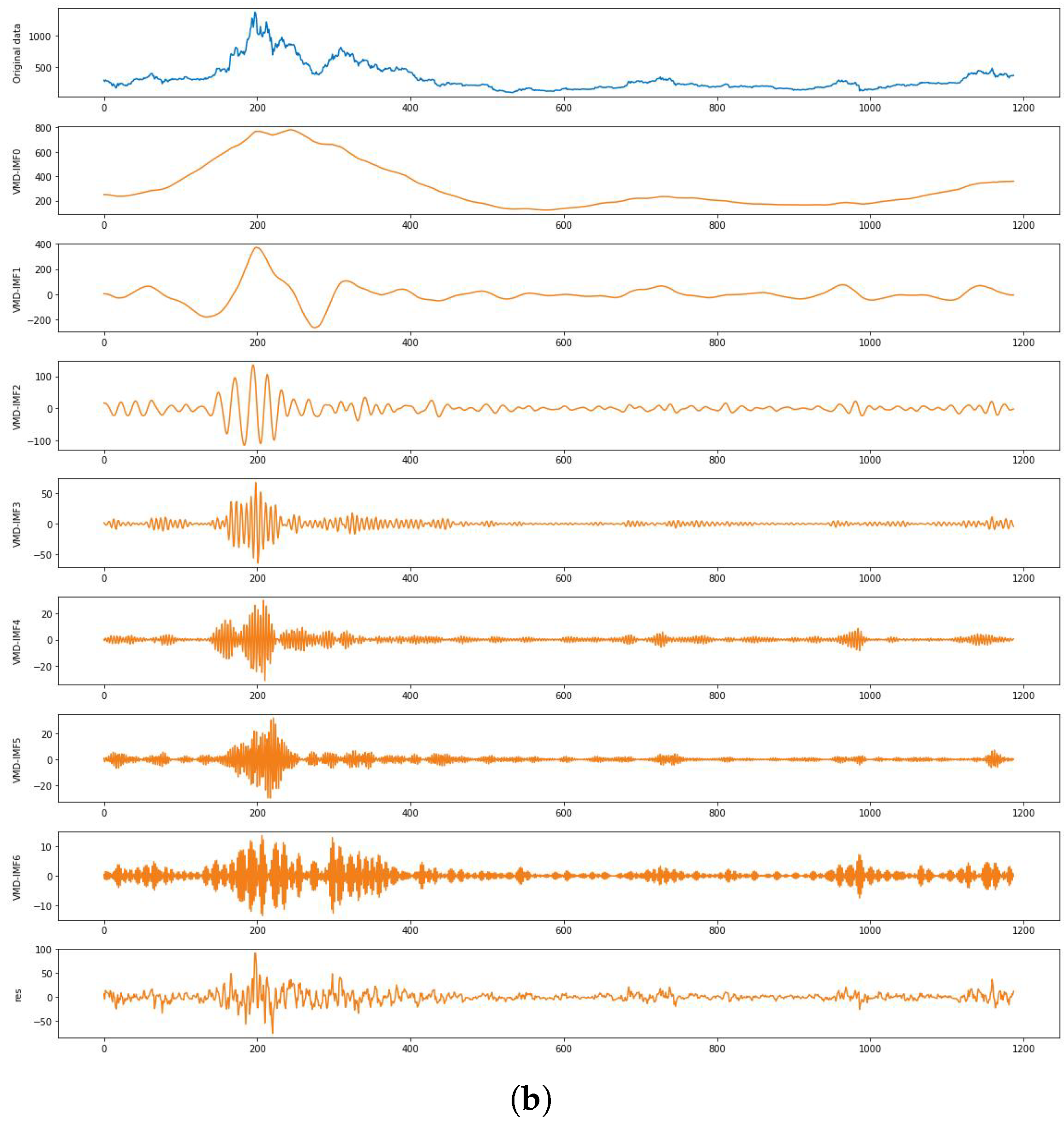
The following figure shows the VMD decomposition results (Figure 8).

4.2. Comparison of Models

There have been too many studies showing that deep learning models like the LSTM model and the GRU model can achieve higher accuracy than the traditional statistical model and machine learning model. This study focuses on comparing the effects of different deep learning models instead of repeating the experiment of the traditional model [6,8].

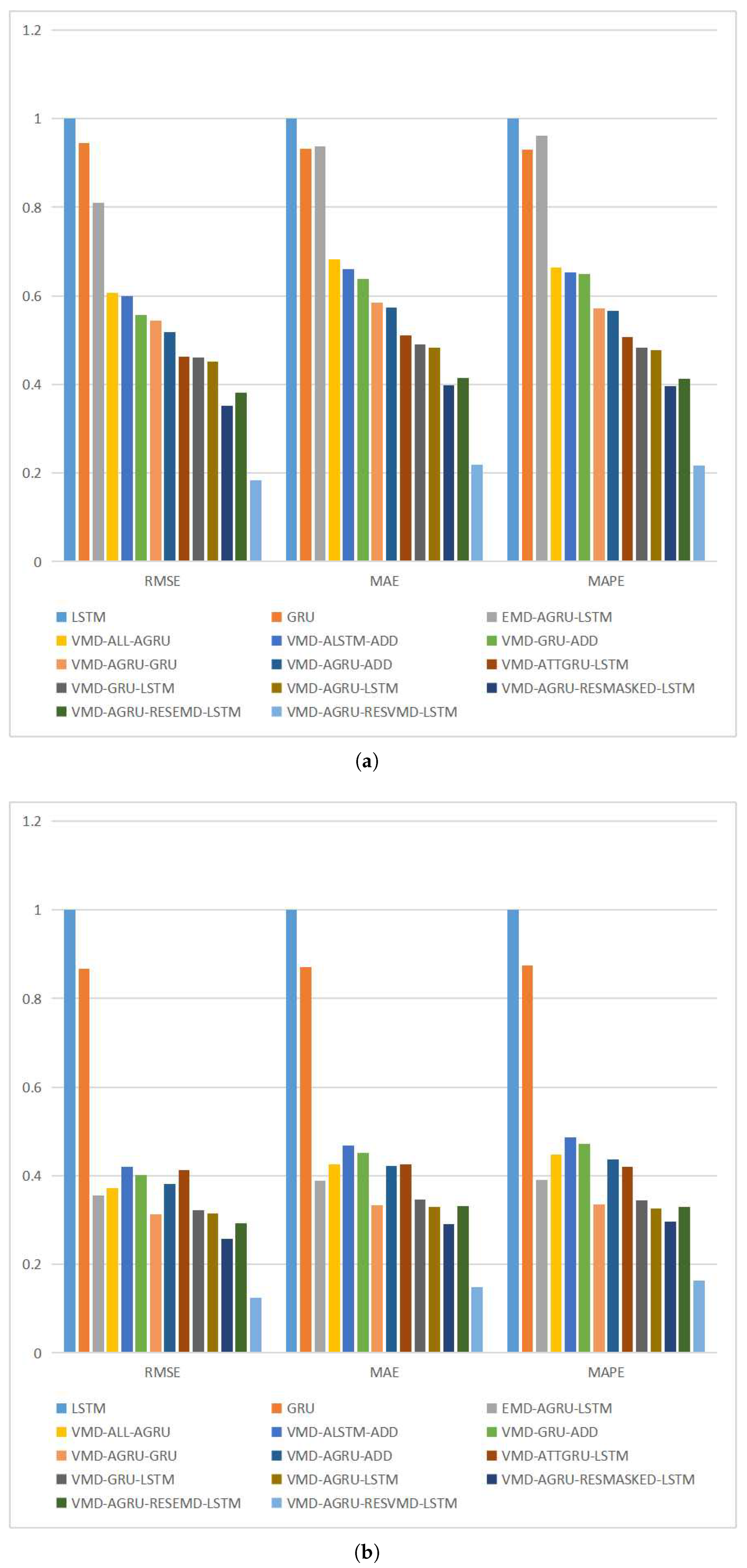
In order to verify the performance of our proposed method, this study compares the prediction effects of other models shown in

Table 1. Prediction results of BTC.

BTC	RMSE	MAE	MAPE
ARIMA	253.051	172.681	0.0161
RF	372.773	283.246	0.0278
SVM	330.389	236.284	0.0223
Informer	333.124	257.918	0.0248
Autoformer	402.196	319.257	0.0308
LSTM	275.958	193.817	0.0182
GRU	260.502	180.501	0.0169
EMD-AGRU-LSTM	223.556	181.721	0.0175
VMD-ALL-AGRU	167.144	132.127	0.0121
VMD-ALSTM-ADD	165.222	127.996	0.0119
VMD-GRU-ADD	153.818	123.571	0.0118
VMD-AGRU-GRU	150.032	113.320	0.0104
VMD-AGRU-ADD	142.985	110.965	0.0103
VMD-ATTGRU-LSTM	127.837	98.901	0.0092
VMD-GRU-LSTM	127.284	94.895	0.0088
VMD-AGRU-LSTM	124.657	93.756	0.0087
VMD-AGRU-RESMASKED-LSTM	97.040	76.951	0.0072
VMD-AGRU-RESEMD-LSTM	105.130	80.417	0.0075
VMD-AGRU-RESVMD-LSTM	50.651	42.298	0.0039

and

Table 2. Prediction results of ETH.

ETH	RMSE	MAE	MAPE
ARIMA	15.979	11.205	0.0321
RF	17.751	12.089	0.0387
SVM	18.549	12.350	0.0381
Informer	24.685	19.666	0.0556
Autoformer	35.633	27.642	0.0831
LSTM	23.129	16.126	0.0462
GRU	20.062	14.054	0.0404
EMD-AGRU-LSTM	8.238	6.269	0.0181
VMD-ALL-AGRU	8.619	6.870	0.0207
VMD-ALSTM-ADD	9.724	7.558	0.0225
VMD-GRU-ADD	9.286	7.287	0.0212
VMD-AGRU-GRU	7.241	5.378	0.0155
VMD-AGRU-ADD	8.840	6.813	0.0202
VMD-ATTGRU-LSTM	9.546	6.867	0.0194
VMD-GRU-LSTM	7.469	5.570	0.0160
VMD-AGRU-LSTM	7.265	5.313	0.0151
VMD-AGRU-RESMASKED-LSTM	5.974	4.677	0.0137
VMD-AGRU-RESEMD-LSTM	6.776	5.351	0.0152
VMD-AGRU-RESVMD-LSTM	2.873	2.410	0.0076

, including a single model, different modal decomposition methods, different component forecasting models, different integration methods, and different treatments of residuals on price forecasting accuracy (Figure 9).

Compared with other models, the proposed VMD-AGRU-RESVMD-LSTM model has the smallest RMSE, MAE, and MAPE and the highest accuracy on the two cryptocurrency datasets of Bitcoin and Ethereum. The DM test is conducted on the prediction results, and the research puts forward that the difference between the model and other models in the price prediction of Bitcoin and Ethereum is significant.

Using the LSTM model as the benchmark model for comparison in the following pictures, $RMS{E}_i=\frac{RMS{E}_i}{RMS{E}_{lstm}},MA{E}_i=\frac{MA{E}_i}{MA{E}_{lstm}},$ and $MAP{E}_i=\frac{MAP{E}_i}{MAP{E}_{lstm}}$.

4.2.1. Comparison of Basic Models

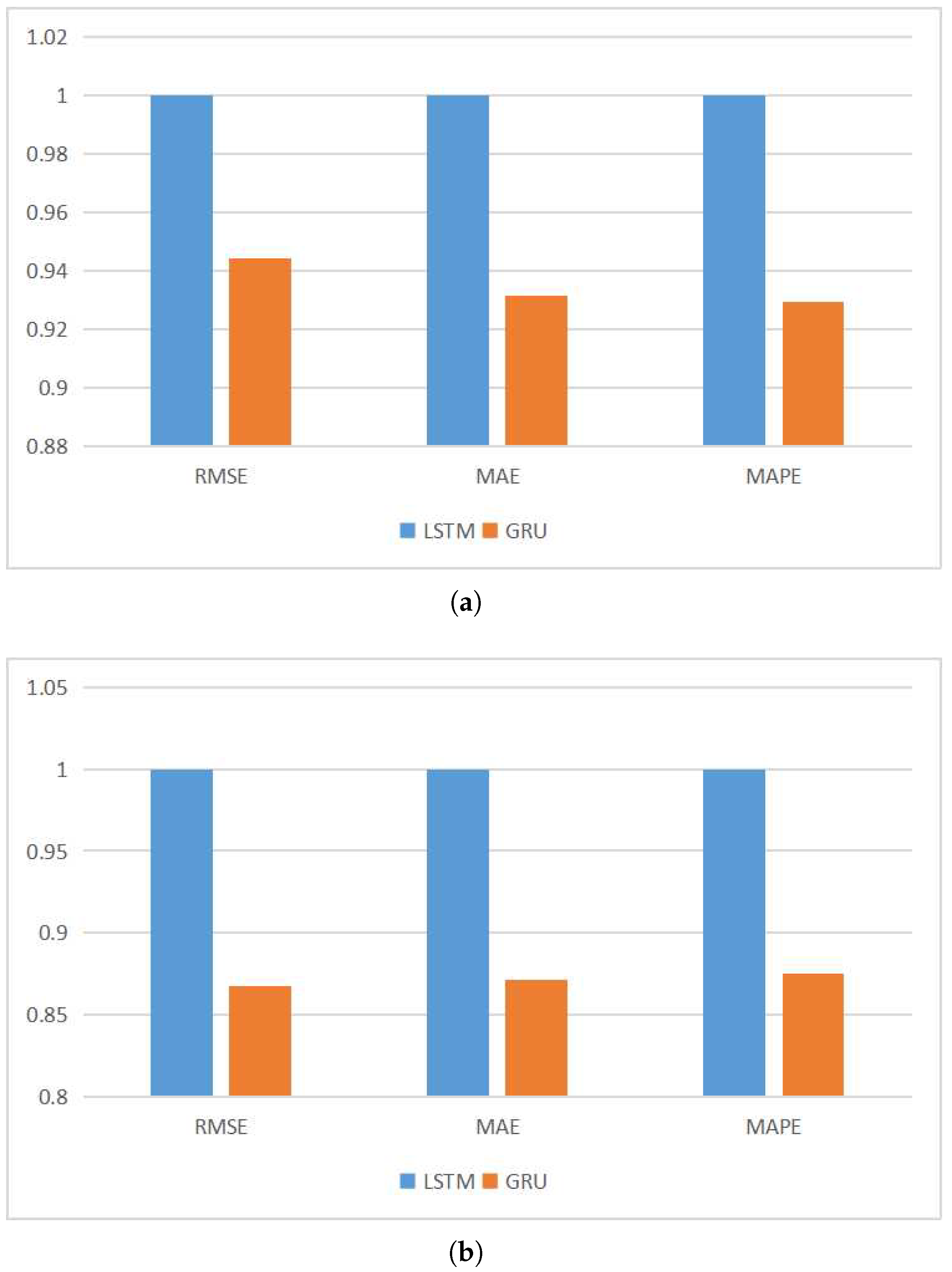
After 100 epochs of operation, the basic LSTM and GRU framework gave relatively stable results, and the average results were obtained after five repeated runs of the model (Figure 10). The RMSE, MAE, and MAPE of the LSTM model on BTC and ETH are 275.958, 193.817, and 0.0182, and 23.129, 16.126, and 0.0462, respectively. The RMSE, MAE, and MAPE of the GRU model on BTC and ETH are 260.502, 180.501, and 0.0169, and 20.062, 14.054, and 0.0404, respectively. Compared with the LSTM model, the GRU model has smaller RMSE, MAE, and MAPE and higher accuracy in predicting the price of Bitcoin and Ethereum. Therefore, the GRU model has better performance in cryptocurrency price prediction.

4.2.2. Comparison of Different Models of Decomposition Methods

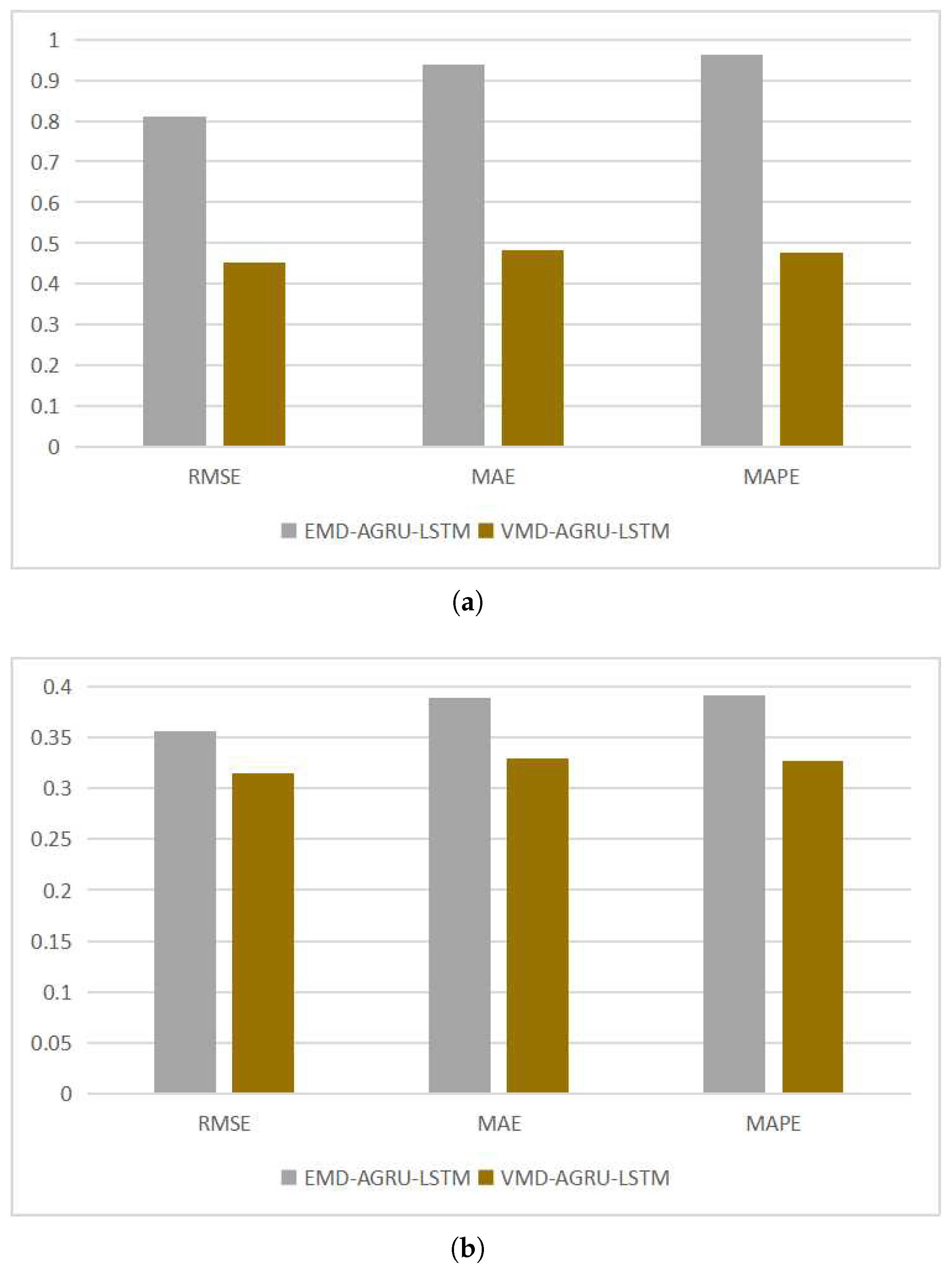
In the BTC dataset, the RMSE, MAE, and MAPE of the VMD-AGRU-LSTM model are 124.657, 93.756, and 0.0087, respectively (Figure 11). The RMSE, MAE, and MAPE of the EMD-AGRU-LSTM model are 223.556, 181.721, and 0.0175, respectively. The RMSE, MAE, and MAPE of the VMD method were reduced by 44.2%, 48.4%, and 50.2% compared with the EMD method.

In the ETH dataset, the RMSE, MAE, and MAPE of the VMD-AGRU-LSTM model are 7.265, 5.313, and 0.0151, respectively. The RMSE, MAE, and MAPE of the EMD-AGRU-LSTM model are 8.238, 6.269, and 0.0181, respectively. The RMSE, MAE, and MAPE of the VMD method were reduced by 11.8%, 15.2%, and 16.6% compared with the EMD method.

The prediction accuracy of the above two decomposition models is significantly improved over that of the single model.

The decomposition of target sequences using the VMD method has smaller RMSE, MAE, and MAPE and higher accuracy than the decomposition using the EMD method on the Bitcoin and Ethereum cryptocurrency datasets.

In summary, the VMD method is selected as the decomposition method of the final mixed model.

4.2.3. Comparison of Different Models of Processing Mode Components

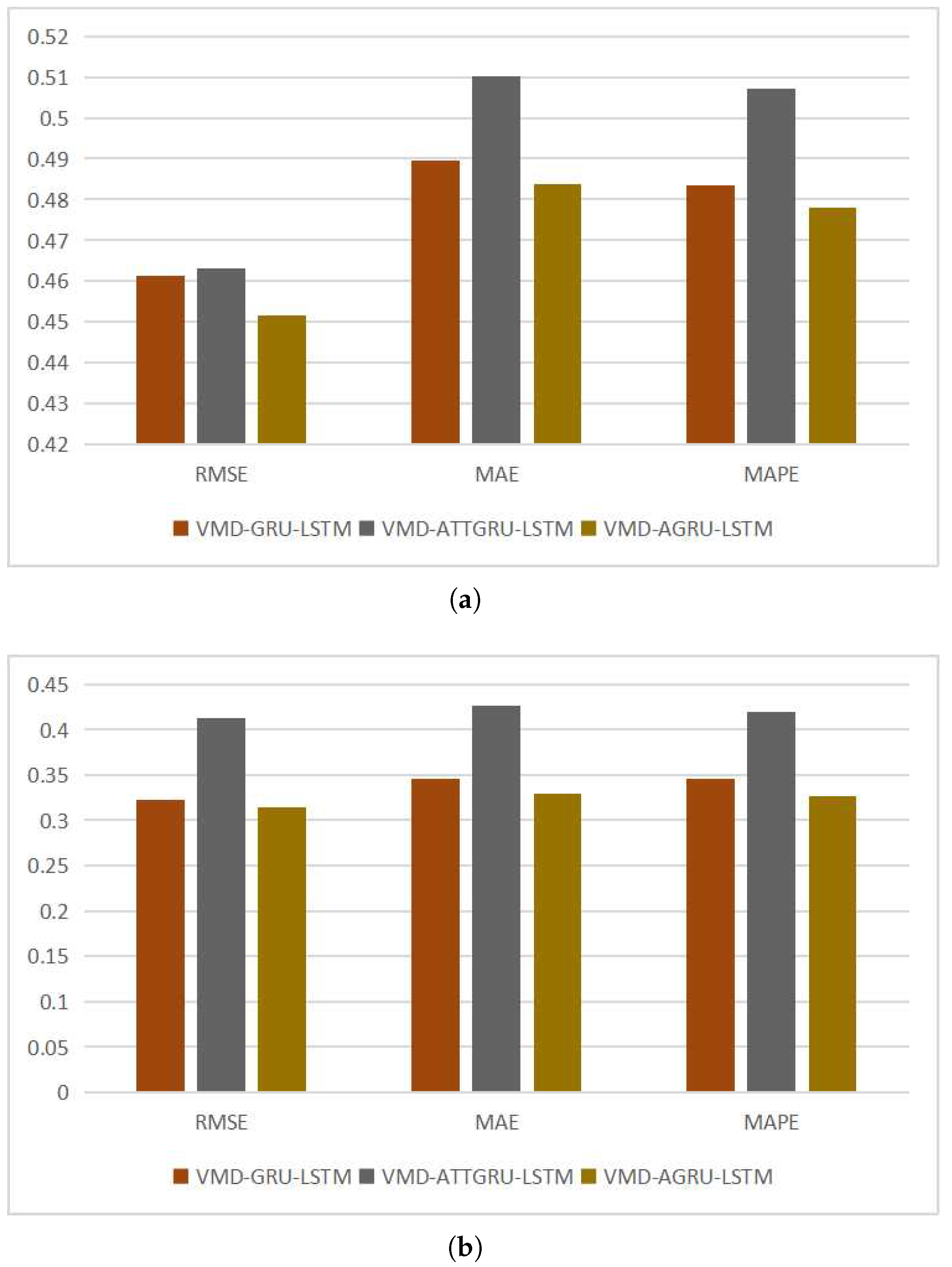
In the BTC dataset, the RMSE, MAE, and MAPE of the VMD-AGRU-LSTM model are 124.657, 93.756, and 0.0087, respectively. The RMSE, MAE, and MAPE of the VMD-ATTGRU-LSTM model are 127.837, 98.901, and 0.0092, respectively. The RMSE, MAE, and MAPE of the VMD-GRU-LSTM model are 127.284, 94.895, and 0.0088, respectively (Figure 12).

In the ETH dataset, the RMSE, MAE, and MAPE of the VMD-AGRU-LSTM model are 7.265, 5.313, and 0.0151, respectively. The RMSE, MAE, and MAPE of the VMD-ATTGRU-LSTM model are 9.546, 6.867, and 0.0194, respectively. The RMSE, MAE, and MAPE of the VMD-GRU-LSTM model are 7.469, 5.570, and 0.0160, respectively.

When the AGRU model proposed in this study is used as the modal component processing model, the integrated model has the smallest RMSE, MAE, and MAPE for both BTC and ETH datasets. The self-attention based ATTGRU model using a self-attention mechanism does not outperform the GRU model in prediction. In summary, the AGRU model is selected as the modal component processing model of the final mixed model.

4.2.4. Comparison of Different Models of Integration Methods

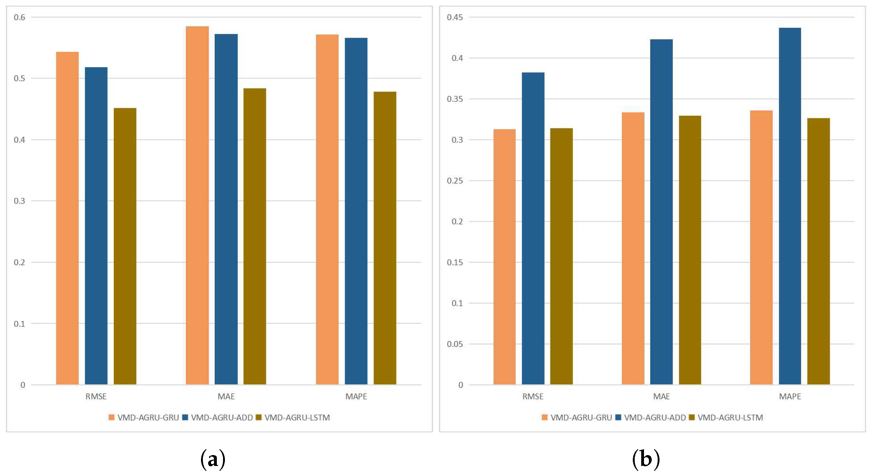
In the BTC dataset, the RMSE, MAE, and MAPE of the VMD-AGRU-LSTM model are 124.657, 93.756, and 0.0087, respectively. The RMSE, MAE, and MAPE of the VMD-AGRU-GRU model are 150.032, 113.320, and 0.0104, and the RMSE, MAE, and MAPE of the VMD-AGRU-ADD model are 142.985, 110.965, and 0.0103, respectively (Figure 13). The LSTM method had a 16.9%, 17.3%, and 16.3% reduction in RMSE, MAE, and MAPE compared with the ADD method and a 12.8%, 15.5%, and 15.6% reduction in RMSE, MAE, and MAPE compared with the GRU method.

In the ETH dataset, the RMSE, MAE, and MAPE of the VMD-AGRU-LSTM model are 7.265, 5.313, and 0.0151, respectively. The RMSE, MAE, and MAPE of the VMD-AGRU-GRU model are 7.241, 5.378, and 0.0155, and the RMSE, MAE, and MAPE of the VMD-AGRU-ADD model are 8.840, 6.813, and 0.0202, respectively. The LSTM method had in imperceptible reduction in RMSE, MAE, and MAPE compared with the GRU method and a 17.8%, 22.0%, and 25.2% reduction in RMSE, MAE, and MAPE compared with the ADD method.

Compared with the model prediction results shown above, when the LSTM network is used as the model integration method, the integrated model has the smallest RMSE, MAE, and MAPE for both BTC and ETH datasets. When the GRU network is used as the integration method, the average RMSE, MAE, and MAPE in the two datasets are smaller than the linear integration method but larger than the RMSE, MAE, and MAPE in the LSTM network. This result shows that the integration using the deep learning method has higher prediction accuracy than the integration using a linear method, and the integration using LSTM has higher prediction accuracy than the integration using the GRU method. In summary, the LSTM model is selected as the integration method for the final hybrid model.

4.2.5. Comparison of Different Models of Residual Processing Methods

At present, there is a lack of relevant research on the treatment of residuals in the decomposition ensemble prediction. Some studies regard residuals as the input model of high-frequency modal components, while the remaining studies directly discard the residuals. However, if the residuals are directly discarded, the sum of modal components will not be equal to the original sequence (Figure 14).

In the BTC dataset, the RMSE, MAE, and MAPE of the VMD-AGRU-LSTM model are 124.657, 93.756, and 0.0087, respectively. The RMSE, MAE, and MAPE of the VMD-AGRU-RESMASKED-LSTM model are 97.040, 76.951, and 0.0072; the RMSE, MAE, and MAPE of the VMD-AGRU-RESEMD-LSTM model are 105.130, 80.417, and 0.0075; and the RMSE, MAE, and MAPE of the VMD-AGRU-RESVMD-LSTM model are 50.651, 42.298, and 0.0039, respectively.

In the ETH dataset, the RMSE, MAE, and MAPE of the VMD-AGRU-LSTM model are 7.265, 5.313, and 0.0151, respectively. The RMSE, MAE, and MAPE of the VMD-AGRU-RESMASKED-LSTM model are 5.974, 4.677, and 0.0137; the RMSE, MAE, and MAPE of the VMD-AGRU-RESEMD-LSTM model are 6.776, 5.351, and 0.0152; and the RMSE, MAE, and MAPE of the VMD-AGRU-RESVMD-LSTM model are 2.873, 2.410, and 0.0076, respectively.

The residual proposed in this study is predicted to have the smallest RMSE, MAE, and MAPE in BTC and ETH datasets using the VMD method in the decomposition ensemble. Considering residuals as high-frequency modal components, the input model is larger than RMSE, MAE, and MAPE, which directly discard residuals. Therefore, directly discarding residuals has higher accuracy compared to taking them as modal components. The prediction performance of the model is not improved by residual EMD redecomposition. In summary, the residual VMD redecomposition method was selected as the residual processing method of the final mixed model.

4.3. Robustness Test

The study conducted a robustness assessment by employing an alternate dataset. The model was evaluated using daily closing prices of Bitcoin and Ethereum from 1 January 2018 to 18 August 2023. Results presented in

Table 3. Prediction results of BTC (January 2018 to August 2023).

BTC	RMSE	MAE	MAPE
Informer	1881.335	1508.047	0.06695
Autoformer	1382.980	1076.087	0.04687
LSTM	1433.723	1290.773	0.05526
GRU	1374.023	1107.899	0.04597
EMD-AGRU-LSTM	888.160	808.401	0.03399
VMD-ALL-AGRU	1288.820	1232.183	0.05399
VMD-ALSTM-ADD	1219.922	1164.164	0.05110
VMD-GRU-ADD	1194.904	1138.762	0.04995
VMD-AGRU-GRU	619.985	568.955	0.02408
VMD-AGRU-ADD	815.058	735.968	0.03141
VMD-ATTGRU-LSTM	494.428	436.796	0.01921
VMD-GRU-LSTM	446.177	356.374	0.01472
VMD-AGRU-LSTM	438.695	381.154	0.01738
VMD-AGRU-RESMASKED-LSTM	420.418	363.722	0.01611
VMD-AGRU-RESEMD-LSTM	357.822	302.413	0.01364
VMD-AGRU-RESVMD-LSTM	260.727	201.248	0.00843

and

Table 4. Prediction results of ETH (January 2018 to August 2023).

ETH	RMSE	MAE	MAPE
Informer	137.335	108.763	0.06643
Autoformer	114.056	89.348	0.05789
LSTM	114.480	95.815	0.06024
GRU	100.871	86.150	0.05479
EMD-AGRU-LSTM	83.491	73.991	0.04636
VMD-ALL-AGRU	83.958	68.334	0.04176
VMD-ALSTM-ADD	79.020	73.411	0.04683
VMD-GRU-ADD	74.671	62.277	0.03813
VMD-AGRU-GRU	51.470	45.204	0.02881
VMD-AGRU-ADD	68.301	62.309	0.03932
VMD-ALL-AGRU	83.958	68.334	0.04176
VMD-ALSTM-ADD	79.020	73.411	0.04683
VMD-GRU-ADD	74.671	62.277	0.03813
VMD-AGRU-GRU	51.470	45.204	0.02881
VMD-AGRU-ADD	68.301	62.309	0.03932
VMD-ATTGRU-LSTM	59.326	50.420	0.03082
VMD-GRU-LSTM	50.327	39.118	0.02481
VMD-AGRU-LSTM	43.787	37.201	0.02414
VMD-AGRU-RESMASKED-LSTM	34.427	27.660	0.01771
VMD-AGRU-RESEMD-LSTM	37.818	30.899	0.01910
VMD-AGRU-RESVMD-LSTM	25.291	19.348	0.01237

reaffirm that the proposed hybrid model consistently outperforms other benchmark models across distinct time periods. The experimental conclusions remained consistent and unchanged, reinforcing the robustness of the model across various datasets.

4.4. DM Test

Table 5. DM test (p value) of BTC.

	LSTM	GRU	E-AGRU-LSTM	V-ALL-AGRU	V-ALSTM-ADD	V-GRU-ADD	V-AGRU-ADD	V-ATTGRU-LSTM	V-GRU-LSTM	V-AGRU-LSTM	V-AGRU-RMK-LSTM	V-AGRU-REMD-LSTM	V-AGRU-RVMD-LSTM
LSTM
GRU	0.023
E-AGRU-LSTM	0.617	0.892
V-ALL-AGRU	$4.64\times {10}^{-4}$	$1.36\times {10}^{-3}$	$6.78\times {10}^{-6}$
V-ALSTM-ADD	$4.61\times {10}^{-5}$	$2.23\times {10}^{-4}$	$2.94\times {10}^{-5}$	0.928
v-GRU-ADD	0.972	0.675	0.507	$1.15\times {10}^{-4}$	$1.01\times {10}^{-4}$
V-AGRU-ADD	$1.42\times {10}^{-5}$	$7.22\times {10}^{-5}$	$8.77\times {10}^{-5}$	0.815	0.758	$7.66\times {10}^{-13}$
V-ATTGRU-LSTM	$3.63\times {10}^{-7}$	$2.45\times {10}^{-6}$	$6.76\times {10}^{-6}$	0.397	0.331	$2.31\times {10}^{-14}$	0.018
V-GRU-LSTM	$8.04\times {10}^{-10}$	$3.71\times {10}^{-9}$	$7.60\times {10}^{-13}$	$9.42\times {10}^{-5}$	$1.16\times {10}^{-6}$	$9.72\times {10}^{-14}$	$1.52\times {10}^{-3}$	$9.16\times {10}^{-3}$
V-AGRU-LSTM	$8.17\times {10}^{-10}$	$3.42\times {10}^{-9}$	$6.56\times {10}^{-13}$	$8.23\times {10}^{-5}$	$2.35\times {10}^{-6}$	$7.56\times {10}^{-14}$	$1.50\times {10}^{-3}$	$9.02\times {10}^{-3}$	0.972
V-AGRU-RMK-LSTM	$1.25\times {10}^{-10}$	$3.86\times {10}^{-10}$	$3.36\times {10}^{-18}$	$8.73\times {10}^{-12}$	$3.68\times {10}^{-10}$	$3.05\times {10}^{-20}$	$8.77\times {10}^{-7}$	$1.09\times {10}^{-5}$	$1.90\times {10}^{-4}$	$1.40\times {10}^{-4}$
V-AGRU-REMD-LSTM	$5.58\times {10}^{-9}$	$3.19\times {10}^{-8}$	$4.56\times {10}^{-17}$	$4.93\times {10}^{-7}$	$6.86\times {10}^{-6}$	$7.16\times {10}^{-14}$	$1.81\times {10}^{-3}$	$8.84\times {10}^{-3}$	0.288	0.304	0.188
V-AGRU-RVMD-LSTM	$1.16\times {10}^{-16}$	$7.19\times {10}^{-16}$	$6.19\times {10}^{-36}$	$9.99\times {10}^{-24}$	$1.84\times {10}^{-21}$	$3.08\times {10}^{-24}$	$4.88\times {10}^{-19}$	$2.88\times {10}^{-17}$	$3.28\times {10}^{-16}$	$1.38\times {10}^{-15}$	$1.40\times {10}^{-10}$	$5.07\times {10}^{-15}$

and

Table 6. DM test (p value) of ETH.

	LSTM	GRU	E-AGRU-LSTM	V-ALL-AGRU	V-ALSTM-ADD	V-GRU-ADD	V-AGRU-ADD	V-ATTGRU-LSTM	V-GRU-LSTM	V-AGRU-LSTM	V-AGRU-RMK-LSTM	V-AGRU-REMD-LSTM	V-AGRU-RVMD-LSTM
LSTM
GRU	0.014
E-AGRU-LSTM	$1.84\times {10}^{-11}$	$3.70\times {10}^{-10}$
V-ALL-AGRU	$8.76\times {10}^{-8}$	$2.20\times {10}^{-6}$	0.132
V-ALSTM-ADD	$1.26\times {10}^{-28}$	$7.48\times {10}^{-33}$	$3.29\times {10}^{-45}$	$2.86\times {10}^{-40}$
V-GRU-ADD	$2.31\times {10}^{-26}$	$3.49\times {10}^{-31}$	$2.55\times {10}^{-44}$	$3.63\times {10}^{-39}$	$1.05\times {10}^{-20}$
V-AGRU-ADD	$3.37\times {10}^{-27}$	$7.94\times {10}^{-32}$	$5.92\times {10}^{-44}$	$2.28\times {10}^{-39}$	$2.14\times {10}^{-8}$	$1.08\times {10}^{-12}$
V-ATTGRU-LSTM	$8.76\times {10}^{-14}$	$1.70\times {10}^{-12}$	0.031	$1.22\times {10}^{-5}$	$1.22\times {10}^{-46}$	$3.36\times {10}^{-46}$	$9.34\times {10}^{-46}$
V-GRU-LSTM	$1.18\times {10}^{-13}$	$3.99\times {10}^{-12}$	0.096	$5.42\times {10}^{-4}$	$7.48\times {10}^{-46}$	$3.12\times {10}^{-45}$	$7.58\times {10}^{-45}$	0.077
V-AGRU-LSTM	$2.85\times {10}^{-14}$	$8.83\times {10}^{-13}$	0.035	$2.29\times {10}^{-4}$	$3.47\times {10}^{-47}$	$1.19\times {10}^{-46}$	$3.46\times {10}^{-46}$	0.919	0.025
V-AGRU-RMK-LSTM	$3.25\times {10}^{-12}$	$2.98\times {10}^{-11}$	$2.31\times {10}^{-3}$	$1.78\times {10}^{-6}$	$1.42\times {10}^{-46}$	$3.48\times {10}^{-46}$	$7.39\times {10}^{-46}$	0.121	0.048	0.142
V-AGRU-REMD-LSTM	$1.69\times {10}^{-10}$	$1.83\times {10}^{-9}$	0.107	$3.96\times {10}^{-4}$	$1.01\times {10}^{-46}$	$3.03\times {10}^{-46}$	$9.41\times {10}^{-46}$	0.703	0.885	0.747	0.044
V-AGRU-RVMD-LSTM	$1.54\times {10}^{-16}$	$8.74\times {10}^{-16}$	$4.23\times {10}^{-12}$	$9.42\times {10}^{-20}$	$2.21\times {10}^{-49}$	$3.03\times {10}^{-49}$	$1.09\times {10}^{-48}$	$3.82\times {10}^{-9}$	$3.74\times {10}^{-10}$	$8.59\times {10}^{-9}$	$8.51\times {10}^{-9}$	$5.60\times {10}^{-14}$

show p values of the DM tests between Bitcoin models. The p value of the DM test calculated by any other model is less than 0.05. When the p value is less than 0.05, the null hypothesis is rejected, which means that the two models have different effects. The DM test results show that the VMD-AGRU-RESVMD-LSTM model is significantly superior to other models.

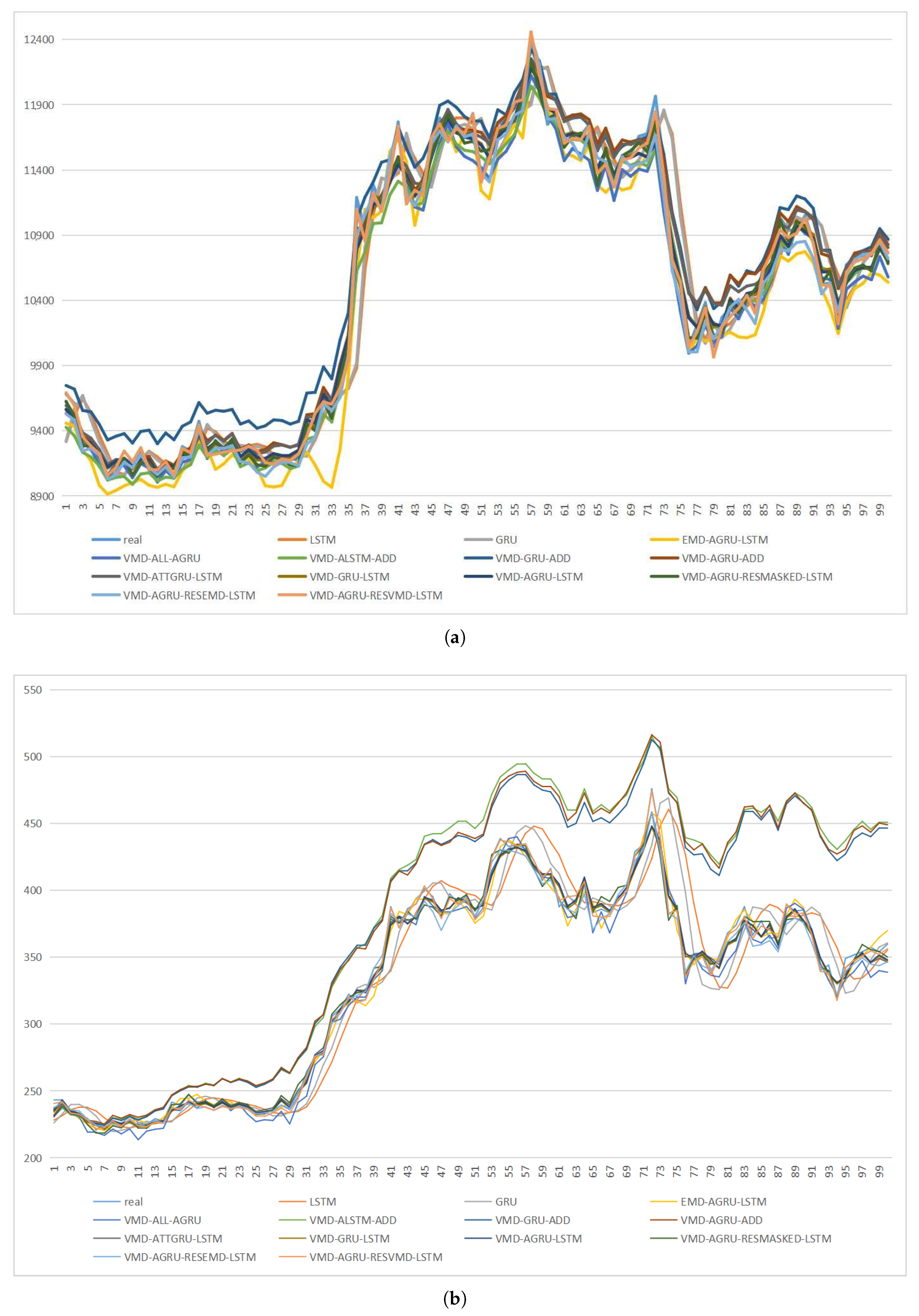
The following figure shows prediction results of $T+1$ of the VMD-AGRU-RESVMD-LSTM model (Figure 15).

4.5. Application of Investment Strategy

In cryptocurrency speculation, investors make investment decisions based on their expectations of future cryptocurrency prices rising and falling. In order to gain income, the company builds a portfolio by forecasting the price of cryptocurrencies, thus achieving profits. Specifically, the model can predict the price of cryptocurrency in the future, calculate the forecast yield according to the forecast results, and construct the corresponding trading decisions to go long or short. The income calculation formula in cryptocurrency speculation is as follows:

$$R_t=\frac{P_t-P_{t-1}-c_t^b·\mathrm{Ind}(\widetilde{P_t}>\widetilde{P_{t-1}}+c_t^b)-c_t^s·\mathrm{Ind}(\widetilde{P_t}<\widetilde{P_{t-1}}+c_t^b)}{P_{t-1}},$$

(12)

where $P_t$ represents the price of cryptocurrency at time t; $c_t^b$ and $c_t^s$ represent the transaction cost when buying and selling at time t, respectively; $\mathrm{Ind}(·)$ is the indication function, which has a value of 1 when the condition in parentheses is true, and 0 otherwise; and $R_t$ represents the yield at time t. Generally, the transaction costs of buying and selling on cryptocurrency trading platforms are the same, and there is a gap between different platforms. A high transaction expense rate of 5% is selected as the transaction cost of the strategy. We construct an investment strategy through VMD-AGRU-RESVMD-LSTM model forecast results shown in

Table 7. Return test of BTC.

	Real Close Price	Real Yield	Forecast Close Price	Forecast Yield	Strategy
1	9680.947		9692.199
2	9609.680	−0.0073616	9593.245	−0.0102097	0
3	9311.136	−0.0310670	9354.024	−0.0249364	0
4	9252.633	−0.0062831	9281.282	−0.0077765	0
5	9171.732	−0.0087436	9225.277	−0.0060342	0
6	9022.154	−0.0163086	9058.503	−0.018078	0
7	9101.850	0.0088334	9118.204	0.0065906	1
8	9188.061	0.0094718	9244.21	0.0138192	0
9	9148.445	−0.0043117	9163.483	−0.0087327	−1
⋯	⋯⋯	⋯⋯	⋯⋯	⋯⋯
96	10,729.067	0.0052575	10693.639	0.0071971	0
97	10,741.476	0.0011564	10,719.955	0.0024609	0
98	10,752.345	0.0010119	10,753.194	0.0031007	0
99	10,863.066	0.0102973	10,862.386	0.0101544	0
100	10,764.284	−0.0090933	10,762.220	−0.0092214	−1

and

Table 8. Return test of ETH.

	Real Close Price	Real Yield	Forecast Close Price	Forecast Yield	Strategy
1	243.316		240.604
2	243.060	−0.0010529	241.994	0.0057772	1
3	234.433	−0.0354915	233.355	−0.0356975	−1
4	232.354	−0.0088690	232.678	−0.0029022	0
5	229.415	−0.0126497	228.062	−0.0198414	0
6	220.756	−0.0377423	221.891	−0.0270529	0
7	224.968	0.0190790	222.556	0.0029944	0
8	227.850	0.0128106	227.614	0.022727	1
9	225.636	−0.00971612	223.418	−0.018433	−1
10	231.030	0.0239050	229.235	0.0260330	1
⋯	⋯⋯	⋯⋯	⋯⋯	⋯⋯
96	351.677	0.0077079	347.582	0.0164573	0
97	354.095	0.0068757	350.895	0.0095302	0
98	357.387	0.0092972	354.708	0.01086734	0
99	353.898	−0.0097628	352.155	−0.0071983	−1
100	359.780	0.0166198	356.284	0.0117264	1

. A strategy of 1 means buy, a strategy of −1 means sell, and a strategy of 0 means no operation.

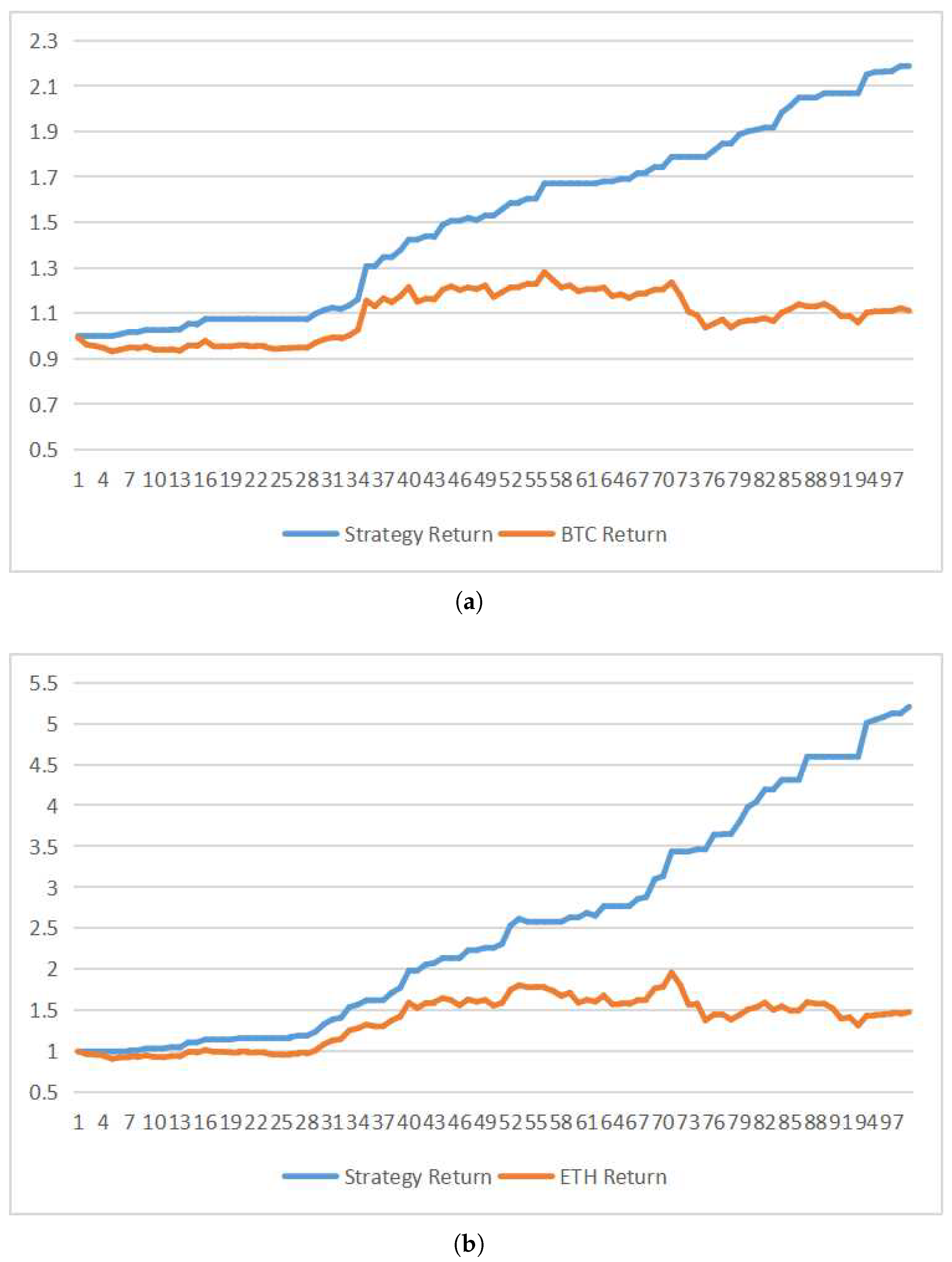
For the portfolio on BTC, the net back-test value is 2.187, and the net market value of BTC is 1.112; for the portfolio on ETH, the net back-test value is 5.204, and the net market value of ETH is 1.479 (Figure 16). These numbers indicate that the predicted results of the proposed model have a good performance in the actual back-test, suggesting that the model has excellent practical significance.

5. Conclusions

In pursuit of achieving excellent and robust predictive performance for Bitcoin price sequences, this paper proposes a hybrid model, VMD-AGRU-RESVMD-LSTM, which integrates the variational mode decomposition (VMD) algorithm, attention mechanism, GRU model, and LSTM model. Additionally, the model incorporates residual sequence re-decomposition as a means of handling residuals resulting from VMD decomposition.

The superiority of GRU in the domain of time series forecasting has been extensively verified through research. However, individual deep learning models struggle to discern the importance of distinct time series features. To enhance the feature recognition ability of the predictive model, the incorporation of an attention mechanism becomes imperative.

In the realm of attention mechanisms, self-attention mechanisms are often employed to identify features within time series. However, for the task of forecasting cryptocurrency price sequences, the effectiveness of such self-attention mechanisms is not optimal. Hence, a more tailored attention mechanism that aligns better with the characteristics of time series data is constructed to synergize with the GRU model.

The exploration of underlying features within time series can significantly enhance predictive performance of models. Therefore, leveraging the capabilities of the VMD algorithm to adeptly uncover these latent features within the original time series is essential. After reviewing numerous related studies, it becomes evident that, despite the respectable performance of decomposition ensemble methods across various problems, these methods exhibit a bias in handling residuals, leading to errors in final predictions. By employing a re-decomposition approach for handling residuals, we mitigate the errors introduced by residuals and further boost predictive performance.

The study conducted a profit and loss back-testing of the proposed model’s predictive results, and the final outcomes demonstrated strong performance in real-world back-testing scenarios. This outcome underscores the practical economic value of the model, as it showcases its efficacy in generating tangible profits and losses, thereby validating its potential impact on investment strategies and decision-making processes.

The experiments focus on the two largest cryptocurrencies, Bitcoin and Ethereum, by evaluating the proposed hybrid model against other models using standard evaluation metrics and DNA tests. By comparing the hybrid model to other models, the results demonstrate that the proposed model outperforms not only basic decomposition ensemble models but also other mainstream models. Furthermore, the experiments confirm the effectiveness of residual re-decomposition in cryptocurrency price sequence prediction and the improvement in predictive performance due to the attention mechanism. The use of VMD decomposition is proven to be more effective than EMD decomposition in uncovering the latent features within time series.

Cryptocurrency price fluctuations are influenced by a multitude of factors, including macroeconomic aspects such as taxes and regulations, investor sentiments, cryptocurrency mining costs, and more. Relying solely on historical data for predictions may not adequately capture the mechanisms through which real-world factors impact cryptocurrency variations. In future research, a multi-modal predictive model for cryptocurrency price forecasting is a potential avenue. This involves incorporating economic indicators, policy indicators, or other time series variables, along with historical cryptocurrency data, as inputs to an extended predictive model. Furthermore, natural language processing (NLP) techniques could be employed to process cryptocurrency-related news texts from the web, extracting market sentiment indicators as additional inputs to the predictive model. This combination of time series and textual data has been shown to enhance prediction accuracy in stock price forecasting, yet such research is relatively scarce in the cryptocurrency domain, making multi-modal cryptocurrency price prediction research highly significant.

Another area of future study involves adapting the existing variational mode decomposition (VMD) algorithm to handle multi-variable decomposition. Since VMD is primarily developed for single-variable decomposition, exploring how existing multi-variable VMD algorithms perform in cryptocurrency prediction scenarios would be valuable.

Optimizing model hyperparameters is also a critical consideration. In this paper, hyperparameter selection was mainly guided by existing research and trial and error. Incorporating suitable hyperparameter optimization algorithms such as particle swarm optimization could enhance the interpretability and effectiveness of the hyperparameter selection process.

Addressing regime change issues in cryptocurrency price prediction is another important aspect. Major external events, such as the COVID-19 pandemic or geopolitical shifts, can disrupt the underlying patterns within cryptocurrency sequences, rendering existing models ineffective. Hence, developing methods to detect regime changes and adapt model structures accordingly to account for new features induced by such changes is crucial for constructing robust cryptocurrency price prediction models.

The predictive accuracy of the cryptocurrency hybrid forecasting model, VMD-AGRU-RESVMD-LSTM, holds great importance for investors, as effective predictions can help mitigate investment losses. Furthermore, the model’s predictive outcomes can serve as valuable references for regulatory bodies in various countries, aiding in the formulation of more rational policies. Confidence among investors and regulatory institutions is pivotal in the financial markets, and this predictive model has the potential to enhance market confidence by providing reliable forecasts.

Lastly, the predictive results of this model can offer insights for diversified asset allocation strategies, thereby enhancing the efficiency of asset management and risk control capabilities. In essence, the utilization of the VMD-AGRU-RESVMD-LSTM hybrid model extends its benefits beyond individual investors to influence regulatory decisions, market confidence, and overall asset management efficiency.

References

1. Corbet, S.; Meegan, A.; Larkin, C.; Lucey, B.; Yarovaya, L. Exploring the dynamic relationships between cryptocurrencies and other financial assets. Econ. Lett. 2018, 165, 28–34. [Google Scholar] [CrossRef]
2. Bouri, E.; Shahzad, S.J.H.; Roubaud, D.; Kristoufek, L.; Lucey, B. Bitcoin, gold, and commodities as safe havens for stocks: New insight through wavelet analysis. Q. Rev. Econ. Financ. 2020, 77, 156–164. [Google Scholar] [CrossRef]
3. Andrianto, Y.; Diputra, Y. The effect of cryptocurrency on investment portfolio effectiveness. J. Financ. Account. 2017, 5, 229–238. [Google Scholar] [CrossRef]
4. Chaim, P.; Laurini, M.P. Volatility and return jumps in bitcoin. Econ. Lett. 2018, 173, 158–163. [Google Scholar] [CrossRef]
5. Cheah, E.T.; Fry, J. Speculative bubbles in Bitcoin markets? An empirical investigation into the fundamental value of Bitcoin. Econ. Lett. 2015, 130, 32–36. [Google Scholar] [CrossRef]
6. McNally, S.; Roche, J.; Caton, S. Predicting the price of bitcoin using machine learning. In Proceedings of the 26th IEEE Euromicro International Conference on Parallel, Distributed and Network-Based Processing (PDP), Coimbatore, India, 25–27 January 2018; pp. 339–343. [Google Scholar]
7. Derbentsev, V.; Datsenko, N.; Stepanenko, O.; Bezkorovainyi, V. Forecasting cryptocurrency prices time series using machine learning approach. In Proceedings of the SHS Web of Conferences; EDP Sciences: Les Ulis, France, 2019; Volume 65, p. 02001. [Google Scholar]
8. Dutta, A.; Kumar, S.; Basu, M. A gated recurrent unit approach to bitcoin price prediction. J. Risk Financ. Manag. 2020, 13, 23. [Google Scholar] [CrossRef]
9. Chen, L.; Chi, Y.; Guan, Y.; Fan, J. A hybrid attention-based EMD-LSTM model for financial time series prediction. In Proceedings of the 2nd IEEE International Conference on Artificial Intelligence and Big Data (ICAIBD), Chengdu, China, 25–28 May 2019; pp. 113–118. [Google Scholar]
10. Cao, J.; Li, Z.; Li, J. Financial time series forecasting model based on CEEMDAN and LSTM. Phys. A Stat. Mech. Appl. 2019, 519, 127–139. [Google Scholar] [CrossRef]
11. Huang, Y.; Deng, Y. A new crude oil price forecasting model based on variational mode decomposition. Knowl.-Based Syst. 2021, 213, 106669. [Google Scholar] [CrossRef]
12. Zhao, L.; Li, Z.; Qu, L.; Zhang, J.; Teng, B. A hybrid VMD-LSTM/GRU model to predict non-stationary and irregular waves on the east coast of China. Ocean. Eng. 2023, 276, 114136. [Google Scholar] [CrossRef]
13. Niu, H.; Xu, K.; Wang, W. A hybrid stock price index forecasting model based on variational mode decomposition and LSTM network. Appl. Intell. 2020, 50, 4296–4309. [Google Scholar] [CrossRef]
14. Yu, L.; Wang, S.; Lai, K.K. Forecasting crude oil price with an EMD-based neural network ensemble learning paradigm. Energy Econ. 2008, 30, 2623–2635. [Google Scholar] [CrossRef]
15. Sheta, A.F.; Ahmed, S.E.M.; Faris, H. A comparison between regression, artificial neural networks and support vector machines for predicting stock market index. Soft Comput. 2015, 7, 2. [Google Scholar]
16. Zhou, F.; Huang, Z.; Zhang, C. Carbon price forecasting based on CEEMDAN and LSTM. Appl. Energy 2022, 311, 118601. [Google Scholar] [CrossRef]
17. Huang, Y.; Dai, X.; Wang, Q.; Zhou, D. A hybrid model for carbon price forecasting using GARCH and long short-term memory network. Appl. Energy 2021, 285, 116485. [Google Scholar] [CrossRef]
18. Rayi, V.K.; Mishra, S.; Naik, J.; Dash, P. Adaptive VMD based optimized deep learning mixed kernel ELM autoencoder for single and multistep wind power forecasting. Energy 2022, 244, 122585. [Google Scholar] [CrossRef]
19. Ribeiro, M.H.D.M.; da Silva, R.G.; Moreno, S.R.; Mariani, V.C.; dos Santos Coelho, L. Efficient bootstrap stacking ensemble learning model applied to wind power generation forecasting. Int. J. Electr. Power Energy Syst. 2022, 136, 107712. [Google Scholar] [CrossRef]
20. Hu, C.; Zhao, Y.; Jiang, H.; Jiang, M.; You, F.; Liu, Q. Prediction of ultra-short-term wind power based on CEEMDAN-LSTM-TCN. Energy Rep. 2022, 8, 483–492. [Google Scholar] [CrossRef]
21. Wu, Y.X.; Wu, Q.B.; Zhu, J.Q. Improved EEMD-based crude oil price forecasting using LSTM networks. Phys. A Stat. Mech. Appl. 2019, 516, 114–124. [Google Scholar] [CrossRef]
22. Yan, R.; Liao, J.; Yang, J.; Sun, W.; Nong, M.; Li, F. Multi-hour and multi-site air quality index forecasting in Beijing using CNN, LSTM, CNN-LSTM, and spatiotemporal clustering. Expert Syst. Appl. 2021, 169, 114513. [Google Scholar] [CrossRef]
23. Zeng, Y.; Chen, J.; Jin, N.; Jin, X.; Du, Y. Air quality forecasting with hybrid LSTM and extended stationary wavelet transform. Build. Environ. 2022, 213, 108822. [Google Scholar] [CrossRef]
24. Yan, B.; Aasma, M. A novel deep learning framework: Prediction and analysis of financial time series using CEEMD and LSTM. Expert Syst. Appl. 2020, 159, 113609. [Google Scholar]
25. Liu, Y.; Yang, C.; Huang, K.; Gui, W. Non-ferrous metals price forecasting based on variational mode decomposition and LSTM network. Knowl.-Based Syst. 2020, 188, 105006. [Google Scholar] [CrossRef]
26. Rezaei, H.; Faaljou, H.; Mansourfar, G. Stock price prediction using deep learning and frequency decomposition. Expert Syst. Appl. 2021, 169, 114332. [Google Scholar] [CrossRef]
27. Premanode, B.; Toumazou, C. Improving prediction of exchange rates using differential EMD. Expert Syst. Appl. 2013, 40, 377–384. [Google Scholar] [CrossRef]
28. Zhang, Z.; Dai, H.N.; Zhou, J.; Mondal, S.K.; García, M.M.; Wang, H. Forecasting cryptocurrency price using convolutional neural networks with weighted and attentive memory channels. Expert Syst. Appl. 2021, 183, 115378. [Google Scholar] [CrossRef]
29. Wątorek, M.; Drożdż, S.; Kwapień, J.; Minati, L.; Oświęcimka, P.; Stanuszek, M. Multiscale characteristics of the emerging global cryptocurrency market. Phys. Rep. 2021, 901, 1–82. [Google Scholar] [CrossRef]
30. James, N. Dynamics, behaviours, and anomaly persistence in cryptocurrencies and equities surrounding COVID-19. Phys. A Stat. Mech. Appl. 2021, 570, 125831. [Google Scholar] [CrossRef]
31. Adrian, T.; Iyer, T.; Qureshi, M.S. Crypto Prices Move More in Sync with Stocks, Posing New Risks. IMF Blog. 2022. Available online: https://blogs.imf.org/2022/01/11/crypto-prices-move-more-in-sync-with-stocks-posing-new-risks (accessed on 11 January 2022).
32. Islam, M.R.; Rashed-Al-Mahfuz, M.; Ahmad, S.; Molla, M.K. Multiband prediction model for financial time series with multivariate empirical mode decomposition. Discret. Dyn. Nat. Soc. 2012, 2012, 593018. [Google Scholar] [CrossRef]
33. Vaswani, A.; Shazeer, N.; Parmar, N.; Uszkoreit, J.; Jones, L.; Gomez, A.N.; Kaiser, Ł.; Polosukhin, I. Attention is all you need. In Proceedings of the Advances in Neural Information Processing Systems 30 (NIPS 2017), Long Beach, CA, USA, 4–9 December 2017; Volume 30. [Google Scholar]
34. Li, S.; Jin, X.; Xuan, Y.; Zhou, X.; Chen, W.; Wang, Y.X.; Yan, X. Enhancing the locality and breaking the memory bottleneck of transformer on time series forecasting. In Proceedings of the 33rd Conference on Neural Information Processing Systems (NeurIPS 2019), Vancouver, BC, Canada, 8–14 December 2019; Volume 32. [Google Scholar]
35. Hochreiter, S.; Schmidhuber, J. Long short-term memory. Neural Comput. 1997, 9, 1735–1780. [Google Scholar] [CrossRef]
36. Cho, K.; Van Merriënboer, B.; Gulcehre, C.; Bahdanau, D.; Bougares, F.; Schwenk, H.; Bengio, Y. Learning phrase representations using RNN encoder-decoder for statistical machine translation. arXiv 2014, arXiv:1406.1078. [Google Scholar]
Figure 1. Long short-term memory.
Fractalfract 07 00708 g001
Figure 2. Gated recurrent unit.
Fractalfract 07 00708 g002
Figure 3. Attention mechanism.
Fractalfract 07 00708 g003
Figure 4. AGRU model.
Fractalfract 07 00708 g004
Figure 5. Flowchart of our model. (a) The structure of the hybrid model; (b) The structure of VMD-AGRU-RESVMD-LSTM.
Fractalfract 07 00708 g005
Figure 6. Statistical test of Bitcoin price.
Fractalfract 07 00708 g006
Figure 7. Statistical test of Ethereum price.
Fractalfract 07 00708 g007
Figure 8. The IMF components of BTC and ETH. (a) BTC; (b) ETH.
Fractalfract 07 00708 g008aFractalfract 07 00708 g008b
Figure 9. Comparison of models of BTC and ETH. (a) BTC; (b) ETH.
Fractalfract 07 00708 g009
Figure 10. Comparison of basic models of BTC and ETH. (a) BTC; (b) ETH.
Fractalfract 07 00708 g010
Figure 11. Comparison of different models of decomposition methods of BTC and ETH. (a) BTC; (b) ETH.
Fractalfract 07 00708 g011
Figure 12. Comparison of different models of processing mode components of BTC and ETH. (a) BTC; (b) ETH.
Fractalfract 07 00708 g012
Figure 13. Comparison of different models of integration methods for BTC and ETH. (a) BTC; (b) ETH.
Fractalfract 07 00708 g013
Figure 14. Comparison of different models of residual processing methods of BTC and ETH. (a) BTC; (b) ETH.
Fractalfract 07 00708 g014
Figure 15. BTC and ETH prediction results of T + 1 of the VMD-AGRU-RESVMD-LSTM model. (a) BTC; (b) ETH.
Fractalfract 07 00708 g015
Figure 16. Strategy net worth versus true net worth. (a) BTC; (b) ETH.
Fractalfract 07 00708 g016