Local Convergence of Traub’s Method and Its Extensions

Abstract

In this article, we examine the local convergence analysis of an extension of Newton’s method in a Banach space setting. Traub introduced the method (also known as the Arithmetic-Mean Newton’s Method and Weerakoon and Fernando method) with an order of convergence of three. All the previous works either used higher-order Taylor series expansion or could not derive the desired order of convergence. We studied the local convergence of Traub’s method and two of its modifications and obtained the convergence order for these methods without using Taylor series expansion. The radii of convergence, basins of attraction, comparison of iterations of similar iterative methods, approximate computational order of convergence (ACOC), and a representation of the number of iterations are provided.

1. Introduction

Many problems in engineering and natural sciences can be modeled into an equation of the form

$$F\left(x\right)=0,$$

(1)

where $F:\mathsf{\Omega }\subseteq X⟶Y$ is a Fréchet differentiable function on a convex subset $\mathsf{\Omega }\subseteq X;X$ and Y are Banach spaces [1]. We are interested in finding the local unique solution of Equation (1). Typically, no analytical or closed-form solution exists in general. Therefore, we turn to iterative methods. Newton’s method, defined as

$$x_{n+1}=x_n-A_n^{-1}F\left(x_n\right),n=0,1,2,\dots ,$$

where $A_n=F^{\prime }\left(x_n\right),$ is very popular. Almost all methods in the literature are some modification or extension of this method; see [2]. Many authors have considered multi-step methods in order to increase efficiency, as well as the order of convergence [3,4,5,6].

Among the multi-step methods, the Mean Newton methods are well studied (see [7]). Traub introduced a modification of Newton’s method in [5] (see also [8]), defined as follows:

$$\begin{array}{cc}\hfill y_n& =x_n-A_n^{-1}F\left(x_n\right)\hfill \\ \hfill x_{n+1}& =x_n-2{\Delta }_n^{-1}F\left(x_n\right),n=0,1,2\cdots ,\hfill \end{array}$$

(2)

where ${\Delta }_n=F^{\prime }\left(x_n\right)+F^{\prime }\left(y_n\right).$ This method, also called the Arithmetic-Mean Newton’s method, has an order of convergence of three. Later, Weerakoon and Fernando [9] approached the method using a trapezoidal approximation of the interpolatory quadrature formula. Frontini and Sormani in [10] showed that this method is one of the most efficient variants of Newton’s method, which uses the quadrature formula. Later, Cordero et al. [11] extended the method defined for $n=1,2,\cdots$ by

$$\begin{array}{cc}\hfill y_n& =x_n-A_n^{-1}F\left(x_n\right)\hfill \\ \hfill z_n& =x_n-2{\Delta }_n^{-1}F\left(x_n\right)\hfill \\ \hfill x_{n+1}& =z_n-F^{\prime }{\left(y_n\right)}^{-1}F\left(z_n\right),\hfill \end{array}$$

(3)

where $F:D\subseteq {\mathbb{R}}^n⟶{\mathbb{R}}^n.$ However, the method used Taylor series expansion and assumed the existence of derivatives up to order six. Sharma and Parhi [12] removed these assumptions and studied this method in Banach spaces. Nevertheless, they were unable to obtain the desired order. Many local convergences, as well as semi-local convergence studies, have been conducted on this method [7,13,14,15].

In this paper, we consider methods (2), (3) and an extension defined for $n=1,2,\cdots$ by

$$\begin{array}{cc}\hfill y_n& =x_n-A_n^{-1}F\left(x_n\right)\hfill \\ \hfill z_n& =x_n-2{\Delta }_n^{-1}F\left(x_n\right)\hfill \\ \hfill x_{n+1}& =z_n-F^{\prime }{\left(z_n\right)}^{-1}F\left(z_n\right).\hfill \end{array}$$

(4)

This method has an order of six. Parhi [15] has used the above extension to obtain an efficient sixth-order method using a linear interpolation of $F^{\prime }\left(z_n\right)$.

Our paper is divided as follows. In Section 2, each method’s preliminary functions, definitions, and auxiliary results are given in order. Some numerical examples to show the radii of convergence, approximate computational order of convergence (ACOC), and an example to illustrate the basins of attractions are given in Section 3. Section 3 also contains a representation of the number of iterations as a heatmap and tables that compare the iterates of methods (2)–(4) with corresponding methods in [16]. Finally, the paper ends with conclusions in Section 4.

2. Main Results

Firstly, we introduce some functions required in the proofs, along with necessary notations and definitions.

Definition 1

([5] Page 9). If for a sequence $\left\{z_n\right\}$ converging to $z^{*},$ there exist some $p\in [0,\infty )$ such that the limit defined as

$$C_p=\underset{n\to \infty }{lim}\frac{\parallel z_{n+1}-z^{*}\parallel }{\parallel z_n-z^{*}{\parallel }^p}$$

exists. Then, p is called the order of convergence of sequence $\left\{z_n\right\}.$

The above definition is somewhat restrictive. Ortega and Rheinboldt discussed a more general concept of R-order and Q-order in [2]. Nevertheless, with an additional condition $0<C_p<\infty$ on $C_p$, there is equivalence between the above definition and $Q-$ and $R-$ orders (see [17,18]).

We use the $R-$ order of convergence defined as follows (see [19,20]).

A sequence $\left\{z_n\right\}$ converges to $z^{*}$ with $R-$order at least p if there are constants $C\in (0,\infty )$ and $\gamma \in (0,1)$ such that

$$\parallel z_{n+1}-z^{*}\parallel \le C{\gamma }^{p^n},n=0,1,2,\dots .$$

(5)

Note that

$$\parallel z_{n+1}-z^{*}\parallel \le c\parallel z_n-z^{*}{\parallel }^p,c>0,n=0,1,2,\dots ,$$

for $p\in \mathbb{N}$ implies (5) provided $\parallel z_0-z^{*}\parallel <1.$

For practical computation of the order of convergence, one may use the Approximate Computational Order of Convergence (ACOC) [21], defined as

$$\begin{array}{c}\hfill ACOC=log\left(\frac{\parallel z_{k+2}-z_{k+1}\parallel }{\parallel z_{k+1}-z_k\parallel }\right)/log\left(\frac{\parallel z_{k+1}-z_k\parallel }{\parallel z_k-z_{k-1}\parallel }\right).\end{array}$$

Throughout this paper, the open and closed balls centered at $\tilde{u}$ with radius $\delta$ are denoted as

$$\begin{array}{c}\hfill B(\tilde{u},\delta )=\{u\in X:\parallel u-\tilde{u}\parallel <\delta \}\mathrm{and}B[\tilde{u},\delta ]=\{u\in X:\parallel u-\tilde{u}\parallel \le \delta \},\end{array}$$

respectively. Furthermore, $\parallel x_n-x^{*}\parallel$ is denoted by ${ϵ}_{x_n}$, $\parallel y_n-x^{*}\parallel$ is denoted by ${ϵ}_{y_n}$, and $\parallel z_n-x^{*}\parallel$ is denoted by ${ϵ}_{z_n}.$ Let $K_1,K_2$ and M be positive constants in $\mathbb{R}$; our proofs are subject to the following conditions.

Assumption 1.

Assume

 1.

$x^{*}$ is the root of $F\left(x\right)=0$ and $A_{*}^{-1}$ exists, where $A_{*}=F^{\prime }\left(x^{*}\right).$

 2.

There exists $K_1>0,$ such that $\parallel A_{*}^{-1}\left(F^{\prime }\left(x\right)-F^{\prime }\left(y\right)\right)\parallel \le K_1\parallel x-y\parallel$ for all $x,y\in \mathsf{\Omega }.$

 3.

There exists $M>0,$ such that $\parallel A_{*}^{-1}{F}^{″}\left(x\right)\parallel \le M.$

 4.

There exists $K_2>0,$ such that $\parallel A_{*}^{-1}(F^{″}\left(x\right)-F^{″}\left(y\right))\parallel \le K_2\parallel x-y\parallel$ for all $x,y\in \mathsf{\Omega }.$

First, we define function ${\zeta }_1:[0,\frac{1}{K_1})⟶\mathbb{R}$ as

$$\begin{array}{cc}\hfill {\zeta }_1\left(t\right)& =\frac{K_1}{2(1-K_{1}t)}.\hfill \end{array}$$

(6)

Let ${\rho }_1=\frac{2}{3K_1}.$ Note that $h_1\left(t\right):={\zeta }_1\left(t\right)t$ is an increasing function in the interval $[0,\frac{1}{K_1}).$ Furthermore, $h_1\left(0\right)=0$ and $h_1\left({\rho }_1\right)=1.$ That is,

$$\begin{array}{c}\hfill 0\le {\zeta }_1\left(t\right)t<1\forall t\in [0,{\rho }_1).\end{array}$$

(7)

Define ${\zeta }_2:[0,{\rho }_1)⟶\mathbb{R}$ as below.

$$\begin{array}{cc}\hfill {\zeta }_2\left(t\right)& =\frac{K_1}{2}(1+{\zeta }_1\left(t\right)t)t.\hfill \end{array}$$

(8)

Let

$$\begin{array}{c}\hfill h_2\left(t\right)={\zeta }_2\left(t\right)-1.\end{array}$$

Clearly, since $h_2\left(0\right)=-1$ and $h_2\left(t\right)⟶\infty$ as $t⟶{\frac{1}{K_1}}^{-}$, by the intermediate value theorem, there exist a smallest positive root for $h_2\left(t\right)$, say ${\rho }_2,$ in the interval $[0,\frac{1}{K_1}).$ So,

$$\begin{array}{c}\hfill 0\le {\zeta }_2\left(t\right)t<1\forall t\in [0,{\rho }_2).\end{array}$$

(9)

Consider, ${\zeta }_3:[0,{\rho }_2)⟶\mathbb{R},$

$$\begin{array}{c}\hfill {\zeta }_3\left(t\right)=\frac{1}{2(1-{\zeta }_2\left(t\right))}\left[M{\zeta }_1\left(t\right)+\frac{K_2}{12}\left(1+\frac{K_1}{2}t\right)\right].\end{array}$$

(10)

Let

$$\begin{array}{c}\hfill h_3\left(t\right)={\zeta }_3\left(t\right)t^2-1.\end{array}$$

Note that $h_3\left(0\right)=-1$ and $h_3\left(t\right)⟶\infty$ as $t⟶{\rho }_2^{-}.$ Intermediate value theorem guarantees a smallest positive root ${\rho }_3$ in $[0,{\rho }_2)$ such that

$$\begin{array}{c}\hfill 0\le {\zeta }_3\left(t\right)<1\forall t\in [0,{\rho }_3).\end{array}$$

(11)

Let

$$R=min\{{\rho }_1,{\rho }_3,1\},$$

(12)

then

$$\begin{array}{c}\hfill 0\le {\zeta }_1\left(t\right)t<1,0\le {\zeta }_2\left(t\right)<1\mathrm{and}0\le {\zeta }_3\left(t\right)t^2<1\forall t\in [0,R).\end{array}$$

(13)

Furthermore, one can see that ${\zeta }_3\left(t\right)$ is an increasing function in $[0,{\rho }_2)$ and hence

$$\begin{array}{c}\hfill {\zeta }_3\left(t\right)\le {\zeta }_3\left(R\right)\forall t\in [0,R).\end{array}$$

(14)

Theorem 1.

Let Assumption hold and let R be as in (12); then the sequence $\left\{x_n\right\}$ defined by (2) with $x_0\in B(x^{*},R)-\left\{x^{*}\right\},$ converges to $x^{*}$ such that

$${ϵ}_{x_{n+1}}\le {\zeta }_3\left(R\right){ϵ}_{x_n}^3,$$

(15)

where ${\zeta }_3$ is as defined in $\left(10\right).$

Proof. 

First, we will show that $F^{\prime }{\left(x_0\right)}^{-1}$ is bounded. Using Assumption 1 and (12),

$$\begin{array}{c}\hfill \parallel A_{*}^{-1}(F^{\prime }\left(x_0\right)-A_{*})\parallel \le K_1{ϵ}_{x_0}\le K_{1}R<1.\end{array}$$

Hence, by Banach’s lemma on invertible operators [22], $F^{\prime }{\left(x_0\right)}^{-1}$ is invertible and

$$\begin{array}{c}\hfill \parallel F^{\prime }{\left(x_0\right)}^{-1}{A}_{*}\parallel \le \frac{1}{1-K_1{ϵ}_{x_0}}.\end{array}$$

(16)

From $\left(2\right)$, we have

$$\begin{array}{cc}\hfill y_0-x^{*}& =x_0-x^{*}-F^{\prime }{\left(x_0\right)}^{-1}F\left(x_0\right)\hfill \\ \hfill & =x_0-x^{*}+F^{\prime }{\left(x_0\right)}^{-1}\left(F\left(x_0\right)-F\left(x^{*}\right)\right)\hfill \\ \hfill & =F^{\prime }{\left(x_0\right)}^{-1}{A}_{*}\left[A_{*}^{-1}{\int }_0^1(F^{\prime }\left(x_0\right)-F^{\prime }(x^{*}+t(x_0-x^{*})))dt(x_0-x^{*})\right],\hfill \end{array}$$

hence, by Assumption 1, Equations (13) and (16),

$$\begin{array}{cc}\hfill {ϵ}_{y_0}& \le ∥F^{\prime }{\left(x_0\right)}^{-1}{A}_{*}\left[{\int }_0^1{A}_{*}^{-1}(F^{\prime }\left(x_0\right)-F^{\prime }(x^{*}+t(x_0-x^{*})))dt(x_0-x^{*})\right]∥\hfill \\ \hfill & \le \parallel F^{\prime }{\left(x_0\right)}^{-1}{A}_{*}\parallel {\int }_0^1{K}_1\parallel x_0-x^{*}-t(x_0-x^{*})\parallel dt{ϵ}_{x_0}\hfill \\ \hfill & \le \frac{K_1}{2(1-K_1{ϵ}_{x_0})}{ϵ}_{x_0}^2\hfill \\ \hfill & \le {\zeta }_1\left({ϵ}_{x_0}\right){ϵ}_{x_0}^2\hfill \\ \hfill & <{ϵ}_{x_0}<R,\hfill \end{array}$$

(17)

so, iterate $y_0\in B(x^{*},R).$ Next, we employ Banach’s lemma of invertible operators [22], Equation (13), and Assumption 1 to show that ${\Delta }_0^{-1}$ is bounded.

$$\begin{array}{cc}\hfill \parallel {\left(2A_{*}\right)}^{-1}({\Delta }_0-2A_{*})\parallel & \le \frac{1}{2}\parallel A_{*}^{-1}(F^{\prime }\left(x_0\right)-A_{*}+F^{\prime }\left(y_0\right)-A_{*})\parallel \hfill \\ \hfill & \le \frac{1}{2}(K_1{ϵ}_{x_0}+K_1{ϵ}_{y_0})\hfill \\ \hfill & \le \frac{K_1}{2}(1+{\zeta }_1\left({ϵ}_{x_0}\right){ϵ}_{x_0}){ϵ}_{x_0}\hfill \\ \hfill & ={\zeta }_2\left({ϵ}_{x_0}\right)<1.\hfill \end{array}$$

So, ${\Delta }_0^{-1}$ is bounded and

$$\begin{array}{cc}\hfill \parallel {\Delta }_0^{-1}{A}_{*}\parallel & \le \frac{1}{2(1-{\zeta }_2\left({ϵ}_{x_0}\right))}.\hfill \end{array}$$

(18)

From (2),

$$\begin{array}{cc}\hfill x_1-x^{*}& =x_0-x^{*}-2{\Delta }_0^{-1}F\left(x_0\right)\hfill \\ \hfill & ={\Delta }_0^{-1}\left[(F^{\prime }\left(x_0\right)+F^{\prime }\left(y_0\right))(x_0-x^{*})-2(F\left(x_0\right)-F\left(x^{*}\right))\right]\hfill \\ \hfill & ={\Delta }_0^{-1}\left[{\int }_0^1(F^{\prime }\left(x_0\right)-F^{\prime }(x^{*}+t(x_0-x^{*})))dt(x_0-x^{*})\right.+\hfill \\ & \left.{\int }_0^1(F^{\prime }\left(y_0\right)-F^{\prime }(x^{*}+t(x_0-x^{*})))dt(x_0-x^{*})\right]\hfill \\ \hfill & ={\Delta }_0^{-1}\left[{\int }_0^1{\int }_0^1{F}^{″}(x^{*}+t(x_0-x^{*})-\theta (x_0-x^{*}-t(x_0-x^{*})))d\theta \right.\hfill \\ & \times (x_0-x^{*}-t(x_0-x^{*}))dt(x_0-x^{*})+{\int }_0^1{\int }_0^1{F}^{″}(x^{*}+t(x_0-x^{*})\hfill \\ & \left.-\theta (y_0-x^{*}-t(x_0-x^{*})))d\theta (y_0-x^{*}-t(x_0-x^{*}))dt\times (x_0-x^{*})\right].\hfill \end{array}$$

Let ${\theta }_{x_0}=\theta (1-t)(x_0-x^{*})$ and ${\theta }_{y_0}=\theta (y_0-x^{*}-t(x_0-x^{*})).$ Now, we split up $x_1-x^{*}$ as follows.

$$\begin{array}{c}\hfill x_1-x^{*}={\Delta }_0^{-1}{A}_{*}[B_1+B_2+B_3],\end{array}$$

(19)

where

$$\begin{array}{cc}\hfill B_1& =A_{*}^{-1}{\int }_0^1{\int }_0^1{F}^{″}(x^{*}+t(x_0-x^{*})-{\theta }_{x_0})d\theta \hfill \\ & \times (1-2t)(x_0-x^{*})dt(x_0-x^{*}),\hfill \\ \hfill B_2& =A_{*}^{-1}{\int }_0^1{\int }_0^1{F}^{″}(x^{*}+t(y_0-x^{*})-{\theta }_{y_0})d\theta (y_0-x^{*})dt(x_0-x^{*}),\hfill \\ \hfill B_3& =A_{*}^{-1}\left[{\int }_0^1{\int }_0^1{F}^{″}(x^{*}+t(x_0-x^{*})-{\theta }_{x_0})d\theta tdt\right.\hfill \\ \hfill & -\left.{\int }_0^1{\int }_0^1{F}^{″}(x^{*}+t(y_0-x^{*})-{\theta }_{y_0})d\theta tdt\right]{(x_0-x^{*})}^2.\hfill \end{array}$$

Using Assumption 1, we have

$$\begin{array}{cc}\hfill \parallel B_1\parallel & \le ∥{\int }_0^1{\int }_0^1{A}_{*}^{-1}{F}^{″}(x^{*}+t(x_0-x^{*})-{\theta }_{x_0})d\theta \hfill \\ & \times (x_0-x^{*}-2t(x_0-x^{*}))dt(x_0-x^{*})\parallel \hfill \\ \hfill & \le ∥\underset{t\in [0,1]}{sup}{\int }_0^1\parallel A_{*}^{-1}{F}^{″}(x^{*}+t(x_0-x^{*})-{\theta }_{x_0})\parallel d\theta \hfill \\ & \times {\int }_0^1\left((1-2t)(x_0-x^{*})\right)dt(x_0-x^{*})∥\hfill \\ \hfill & =0.\hfill \end{array}$$

(20)

In addition, by Assumptions 1 and (17), we have

$$\begin{array}{cc}\hfill \parallel B_2\parallel & =∥{\int }_0^1{\int }_0^1{A}_{*}^{-1}{F}^{″}(x^{*}+t(y_0-x^{*})-{\theta }_{y_0})d\theta (y_0-x^{*})dt(x_0-x^{*})∥\hfill \\ \hfill & \le M{ϵ}_{y_0}{ϵ}_{x_0}\le M{\zeta }_1\left({ϵ}_{x_0}\right){ϵ}_{x_0}^3,\hfill \end{array}$$

(21)

and

$$\begin{array}{cc}\hfill \parallel B_3\parallel & =\parallel {\int }_0^1{\int }_0^1{A}_{*}^{-1}[F^{″}(x^{*}+t(x_0-x^{*})-{\theta }_{x_0})d\theta \hfill \\ & -F^{″}(x^{*}+t(y_0-x^{*})-{\theta }_{y_0})d\theta ]tdt{(x_0-x^{*})}^2\parallel \hfill \\ \hfill & \le K_2{\int }_0^1{\int }_0^{1}t(t-\theta )\parallel x_0-y_0\parallel d\theta dt{ϵ}_{x_0}^2\hfill \\ \hfill & \le \frac{K_2}{12}\parallel x_0-y_0\parallel {ϵ}_{x_0}^2\hfill \\ \hfill & \le \frac{K_2}{12}({ϵ}_{x_0}+{ϵ}_{y_0}){ϵ}_{x_0}^2\hfill \\ \hfill & \le \frac{K_2}{12}\left(1+{\zeta }_1\left({ϵ}_{x_0}\right){ϵ}_{x_0}\right){ϵ}_{x_0}^3.\hfill \end{array}$$

(22)

So, using (19), (20), (21), (22), and (13),

$$\begin{array}{cc}\hfill {ϵ}_{x_1}& \le \parallel {\Delta }_0^{-1}{A}_{*}\parallel \left[M{\zeta }_1\left({ϵ}_{x_0}\right){ϵ}_{x_0}^3+\frac{K_2}{12}(1+{\zeta }_1\left({ϵ}_{x_0}\right){ϵ}_{x_0}){ϵ}_{x_0}^3\right]\hfill \\ \hfill & \le \frac{1}{2(1-{\zeta }_2\left({ϵ}_{x_0}\right))}\left[M{\zeta }_1\left({ϵ}_{x_0}\right)+\frac{K_2}{12}\left(1+\frac{K_1}{2}{ϵ}_{x_0}\right)\right]{ϵ}_{x_0}^3\hfill \\ \hfill & \le {\zeta }_3\left({ϵ}_{x_0}\right){ϵ}_{x_0}^3\hfill \\ \hfill & \le {\zeta }_3\left(R\right)R^2{ϵ}_{x_0}<{ϵ}_{x_0}<R.\hfill \end{array}$$

(23)

Hence, $x_1\in B(x^{*},R)$ and (by (23)) (15) holds for $n=1.$ By induction, the proof is complete if $x_0,y_0,x_1$ are replaced by $x_n,y_n,x_{n+1},$ respectively. □

Next, to provide the convergence analysis of method (3), we define some functions and parameterss below.

Define ${\zeta }_4:[0,\frac{1}{K_1})⟶\mathbb{R}$ by

$$\begin{array}{c}\hfill {\zeta }_4\left(t\right)=K_1{\zeta }_1\left(t\right)t^2.\end{array}$$

(24)

and $h_4:[0,\frac{1}{K_1})⟶\mathbb{R}$

$$\begin{array}{c}\hfill h_4\left(t\right)={\zeta }_4\left(t\right)-1.\end{array}$$

Then, $h_4\left(0\right)=-1$ and $h_4\left(t\right)⟶\infty$ as $t⟶{\frac{1}{K_1}}^{-}.$ Hence, by the intermediate value theorem, $h_4$ has a smallest zero ${\rho }_4\in [0,\frac{1}{K_1}),$ and

$$\begin{array}{c}\hfill 0\le {\zeta }_4\left(t\right)<1\forall t\in [0,{\rho }_4).\end{array}$$

(25)

Define ${\zeta }_5:[0,{\rho }_4)⟶\mathbb{R},$ by

$$\begin{array}{c}\hfill {\zeta }_5\left(t\right)=\frac{K_1}{1-{\zeta }_4\left(t\right)}\left({\zeta }_1\left(t\right)+\frac{1}{2}{\zeta }_3\left(t\right)t\right){\zeta }_3\left(t\right),\end{array}$$

(26)

and $h_5:[0,{\rho }_4)⟶\mathbb{R},$ by

$$\begin{array}{c}\hfill h_5\left(t\right)={\zeta }_5\left(t\right)t^4-1.\end{array}$$

Observe that $h_5\left(0\right)=-1$ and $h_5\left(t\right)⟶\infty$ as $t⟶{\rho }_4^{-}.$ Using the intermediate value theorem, $h_5$ has a smallest zero ${\rho }_5$ in the interval $[0,{\rho }_4).$ Let

$$R_1=min\{R,{\rho }_5\},$$

(27)

then

$$\begin{array}{c}\hfill 0\le {\zeta }_4\left(t\right)<1\mathrm{and}0\le {\zeta }_5\left(t\right)t^4<1\forall t\in [0,R_1).\end{array}$$

(28)

It is clear that ${\zeta }_5$ is an increasing function in $[0,{\rho }_4).$ In particular,

$$\begin{array}{c}\hfill {\zeta }_5\left(t\right)\le {\zeta }_5\left(R_1\right)\forall t\in [0,R_1).\end{array}$$

(29)

Theorem 2.

Let Assumption 1 hold. The sequence $\left\{x_n\right\}$ is as in (3). If $x_0\in B(x^{*},R_1)-\left\{x^{*}\right\},R_1$ is as in (27). Then, the sequence $\left\{x_n\right\}$ converges to $x^{*}$ and

$${ϵ}_{x_{n+1}}\le {\zeta }_5\left(R_1\right){ϵ}_{x_n}^5,$$

(30)

where ${\zeta }_5$ is as defined in (26).

Proof. 

We use induction to prove the theorem. Clearly, one can mimic the proof of Theorem 1 to obtain

$$\begin{array}{c}\hfill {ϵ}_{z_0}\le {\zeta }_3\left({ϵ}_{x_0}\right){ϵ}_{x_0}^3.\end{array}$$

(31)

Now, we will show that $F^{\prime }{\left(y_0\right)}^{-1}$ is bounded using Assumption 1 and (28),

$$\begin{array}{cc}\hfill \parallel A_{*}^{-1}(F\left(y_0\right)-F\left(x^{*}\right))\parallel & \le K_1{ϵ}_{y_0}\hfill \\ \hfill & \le K_1{\zeta }_1\left({ϵ}_{x_0}\right){ϵ}_{x_0}^2\hfill \\ \hfill & ={\zeta }_4\left({ϵ}_{x_0}\right)\le {\zeta }_4\left(R_1\right)<1.\hfill \end{array}$$

Hence, $F^{\prime }{\left(y_0\right)}^{-1}$ is invertible and

$$\begin{array}{c}\hfill \parallel F^{\prime }{\left(y_0\right)}^{-1}{A}_{*}\parallel \le \frac{1}{1-{\zeta }_4\left({ϵ}_{x_0}\right)}.\end{array}$$

(32)

$$\begin{array}{cc}\hfill x_1-x^{*}& =z_0-x^{*}-F^{\prime }{\left(y_0\right)}^{-1}F\left(z_0\right)\hfill \\ \hfill & =z_0-x^{*}-F^{\prime }{\left(y_0\right)}^{-1}[F\left(z_0\right)-F\left(x^{*}\right)]\hfill \\ \hfill & =F^{\prime }{\left(y_0\right)}^{-1}\left[F^{\prime }\left(y_0\right)(z_0-x^{*})-{\int }_0^1{F}^{\prime }(x^{*}+t(z_0-x^{*}))(z_0-x^{*})dt\right]\hfill \\ \hfill & =F^{\prime }{\left(y_0\right)}^{-1}{A}_{*}\left[{\int }_0^1{A}_{*}^{-1}\left((F^{\prime }\left(y_0\right)-F^{\prime }(x^{*}+t(z_0-x^{*})))\right)dt\right](z_0-x^{*}).\hfill \end{array}$$

Hence, by using Assumption 1, (28) and (32), we obtain

$$\begin{array}{cc}\hfill {ϵ}_{x_1}& \le \parallel F^{\prime }{\left(y_0\right)}^{-1}{A}_{*}\parallel {\int }_0^1{K}_1\parallel y_0-x^{*}-t(z_0-x^{*})\parallel dt{ϵ}_{z_0}\hfill \\ \hfill & \le \frac{1}{1-{\zeta }_4\left({ϵ}_{x_0}\right)}{\int }_0^1{K}_1({ϵ}_{y_0}+t{ϵ}_{z_0})dt{ϵ}_{z_0}\hfill \\ \hfill & \le \frac{K_1}{1-{\zeta }_4\left({ϵ}_{x_0}\right)}\left({ϵ}_{y_0}+\frac{{ϵ}_{z_0}}{2}\right){ϵ}_{z_0}\hfill \\ \hfill & \le \frac{K_1}{1-{\zeta }_4\left({ϵ}_{x_0}\right)}\left({\zeta }_1\left({ϵ}_{x_0}\right){ϵ}_{x_0}^2+\frac{1}{2}{\zeta }_3\left({ϵ}_{x_0}\right){ϵ}_{x_0}^3\right)\times {\zeta }_3\left({ϵ}_{x_0}\right){ϵ}_{x_0}^3\hfill \\ \hfill & \le \frac{K_1}{1-{\zeta }_4\left({ϵ}_{x_0}\right)}\left({\zeta }_1\left({ϵ}_{x_0}\right)+\frac{1}{2}{\zeta }_3\left({ϵ}_{x_0}\right){ϵ}_{x_0}\right){\zeta }_3\left({ϵ}_{x_0}\right){ϵ}_{x_0}^5\hfill \\ \hfill & \le {\zeta }_5\left({ϵ}_{x_0}\right){ϵ}_{x_0}^5\hfill \\ \hfill & <{ϵ}_{x_0}<R_1.\hfill \end{array}$$

(33)

I.e., $x_1\in B(x^{*},R_1)$, and from (33) and (29),

$$\begin{array}{cc}\hfill {ϵ}_{x_1}& \le \frac{K_1}{1-{\zeta }_4\left({ϵ}_{x_0}\right)}\left({\zeta }_1\left({ϵ}_{x_0}\right){ϵ}_{x_0}^2+\frac{1}{2}{\zeta }_3\left({ϵ}_{x_0}\right){ϵ}_{x_0}^3\right){\zeta }_3\left({ϵ}_{x_0}\right){ϵ}_{x_0}^3\hfill \\ \hfill & \le \frac{K_1}{1-{\zeta }_4\left({ϵ}_{x_0}\right)}\left({\zeta }_1\left({ϵ}_{x_0}\right)+\frac{1}{2}{\zeta }_3\left({ϵ}_{x_0}\right){ϵ}_{x_0}\right){\zeta }_3\left({ϵ}_{x_0}\right){ϵ}_{x_0}^5\hfill \\ \hfill & \le {\zeta }_5\left({ϵ}_{x_0}\right){ϵ}_{x_0}^5\le {\zeta }_5\left(R_1\right){ϵ}_{x_0}^5.\hfill \end{array}$$

(34)

The rest of the proof follows as in Theorem 1. □

To prove the convergence of method (4), we introduce some more functions and parameters. Let ${\zeta }_6:[0,{\rho }_2)⟶\mathbb{R}$ be defined as

$$\begin{array}{c}\hfill {\zeta }_6\left(t\right)=K_1{\zeta }_3\left(t\right)t^3\end{array}$$

(35)

and $h_6:[0,{\rho }_2)⟶\mathbb{R}$ as

$$\begin{array}{c}\hfill h_6\left(t\right)={\zeta }_6\left(t\right)-1.\end{array}$$

Then, $h_6\left(0\right)=-1$ and $h_6\left(t\right)⟶\infty$ as $t⟶{\rho }_2^{-}.$ By the intermediate value theorem there exists a smallest zero ${\rho }_6$ in the interval $[0,{\rho }_2)$ such that

$$\begin{array}{c}\hfill 0\le {\zeta }_6\left(t\right)<1\forall t\in [0,{\rho }_6).\end{array}$$

(36)

Lastly, we define functions ${\zeta }_7:[0,{\rho }_6)⟶\mathbb{R}$ by

$$\begin{array}{c}\hfill {\zeta }_7\left(t\right)=\frac{K_1}{2(1-{\zeta }_6\left(t\right))}{\zeta }_3^2\left(t\right)\end{array}$$

(37)

and $h_7:[0,{\rho }_6)⟶\mathbb{R}$ by

$$\begin{array}{c}\hfill h_7\left(t\right)={\zeta }_7\left(t\right)t^5-1.\end{array}$$

Then, $h_7\left(0\right)=-1$ and $h_7\left(t\right)⟶\infty$ as $t⟶\infty .$ The intermediate value theorem gives a smallest root ${\rho }_7$ in $[0,{\rho }_6)$ such that

$$\begin{array}{c}\hfill 0\le {\zeta }_7\left(t\right)t^5\le 1\forall t\in [0,{\rho }_7).\end{array}$$

(38)

If

$$R_2=min\{R,{\rho }_7\},$$

(39)

then

$$\begin{array}{c}\hfill 0\le {\zeta }_6\left(t\right)<1\mathrm{and}0\le {\zeta }_7\left(t\right)t^5<1\forall t\in [0,R_2).\end{array}$$

(40)

Furthermore, observe that ${\zeta }_7$ is an increasing function in $[0,{\rho }_6).$ Specifically,

$$\begin{array}{c}\hfill {\zeta }_7\left(t\right)\le {\zeta }_7\left(R_2\right)\forall t\in [0,R_2).\end{array}$$

(41)

Theorem 3.

Let Assumption 1 hold, and the sequence $\left\{x_n\right\}$ defined by (4) with $x_0\in B(x^{*},R_2)-\left\{x^{*}\right\},$ where $R_2$, as in (39), converges to $x^{*}$ such that

$${ϵ}_{x_{n+1}}\le {\zeta }_7\left(R_2\right){ϵ}_{x_n}^6,$$

(42)

where ${\zeta }_7$ is as in (37).

Proof. 

In extension (4), only the last step is different from extension (3). So, we can easily repeat the proof to obtain

$$\begin{array}{c}\hfill {ϵ}_{z_0}\le {\zeta }_3\left({ϵ}_{x_0}\right){ϵ}_{x_0}^3.\end{array}$$

(43)

Now, as in previous case, we will show that $F^{\prime }{\left(z_0\right)}^{-1}$ exists using Assumptions 1 and (40).

$$\begin{array}{cc}\hfill \parallel A_{*}^{-1}(F^{\prime }\left(z_0\right)-A_{*})\parallel & \le K_1{ϵ}_{z_0}\hfill \\ \hfill & \le K_1{\zeta }_3\left({ϵ}_{x_0}\right){ϵ}_{x_0}^3\hfill \\ \hfill & \le {\zeta }_6\left({ϵ}_{x_0}\right)<{\zeta }_6\left(R_2\right)<1.\hfill \end{array}$$

Hence, $F^{\prime }{\left(z_0\right)}^{-1}$ is invertible and

$$\begin{array}{c}\hfill \parallel F^{\prime }{\left(z_0\right)}^{-1}{A}_{*}\parallel \le \frac{1}{1-{\zeta }_6\left({ϵ}_{x_0}\right)}.\end{array}$$

(44)

$$\begin{array}{cc}\hfill x_1-x^{*}& =z_0-x^{*}-F^{\prime }{\left(z_0\right)}^{-1}F\left(z_0\right)\hfill \\ \hfill & =F^{\prime }{\left(z_0\right)}^{-1}\left(F^{\prime }\left(z_0\right)(z_0-x^{*})-{\int }_0^1{F}^{\prime }(x^{*}+t(z_0-x^{*}))(z_0-x^{*})dt\right)\hfill \\ \hfill & =F^{\prime }{\left(z_0\right)}^{-1}{A}_{*}\left({\int }_0^1{A}_{*}(F^{\prime }\left(z_0\right)-F^{\prime }(x^{*}+t(z_0-x^{*})))dt\right)(z_0-x^{*}).\hfill \end{array}$$

Hence, by using (43), Assumptions 1 and (40), it follows that

$$\begin{array}{cc}\hfill {ϵ}_{x_1}& \le \parallel F^{\prime }{\left(z_0\right)}^{-1}{F}^{\prime }(x*)\parallel ∥\left({\int }_0^1{A}_{*}^{-1}(F^{\prime }\left(z_0\right)-F^{\prime }(x^{*}+t(z_0-x^{*})))dt\right)∥{ϵ}_{z_0}\hfill \\ \hfill & \le \frac{1}{1-{\zeta }_6\left({ϵ}_{x_0}\right)}{\int }_0^1{K}_1\left|(1-t)\right|{ϵ}_{z_0}dt{ϵ}_{z_0}\hfill \\ \hfill & \le \frac{K_1}{2(1-{\zeta }_6\left({ϵ}_{x_0}\right))}{\zeta }_3\left({ϵ}_{x_0}\right){ϵ}_{x_0}^3\times {\zeta }_3\left({ϵ}_{x_0}\right){ϵ}_{x_0}^3\hfill \\ \hfill & \le {\zeta }_7\left({ϵ}_{x_0}\right){ϵ}_{x_0}^6\hfill \\ \hfill & <{ϵ}_{x_0}<R_2,\hfill \end{array}$$

(45)

so, $x_1\in B(x^{*},R_2)$. Furthermore, from (41) and (45), we have

$$\begin{array}{cc}\hfill {ϵ}_{x_1}& \le {\zeta }_7\left(R_2\right){ϵ}_{x_0}^6.\hfill \end{array}$$

(46)

Hence, (42) is satisfied for $n=1.$ Now, the proof follows as in Theorem 2. □

The conditions that guarantee a unique solution are given in the following lemma.

Lemma 1.

Suppose Assumption 1 holds and $x^{*}$ is a simple solution of the equation $F\left(x\right)=0.$ Then, $F\left(x\right)=0$ has a unique solution $x^{*}$ in $E:=\mathsf{\Omega }\cap B[x^{*},\overline{r}]$ provided

$$K_1\overline{r}<2.$$

(47)

Proof. 

Let $p\in E$ be such that $F\left(p\right)=0.$ Define $J={\int }_0^1{F}^{\prime }(x^{*}+u(p-x^{*}))du.$ Then, by Assumption 1, we have, in turn

$$\begin{array}{cc}\hfill \parallel A_{*}^{-1}(J-A_{*})\parallel & \le K_1{\int }_0^1\parallel x^{*}+u(p-x^{*})-x^{*}\parallel du\hfill \\ \hfill & \le K_1{\int }_0^{1}u\parallel p-x^{*}\parallel du\hfill \\ \hfill & \le \frac{K_1\overline{r}}{2}<1.\hfill \end{array}$$

It follows that J is invertible, and hence $p=x^{*}$ by the identity $0=F\left(p\right)-F\left(x^{*}\right)=J(p-x^{*}).$ □

3. Illustrations and Numerical Examples

In this section, we will illustrate our results using numerical examples. In the first three examples, we compute the radii of convergence. The next example compares the iterations of methods (2)–(4) with the corresponding methods in [16]. We also compute the ACOC for Examples 2 and 4 (the iterations of Examples 1 and 3 converge within three iterations on almost all initial points, so we have not computed ACOC for these examples). An illustration of the basins of attraction and a representation of the number of iterates as a heatmap follows.

The values of ${\rho }_i,i\in \{1,2,\cdots ,7\}$ for the examples (Examples 1–3) are given in

Table 1. The parameters ${\rho }_i$ of the Examples 1–3.

Example	${\mathit{\rho }}_1$	${\mathit{\rho }}_2$	${\mathit{\rho }}_3$	${\mathit{\rho }}_4$	${\mathit{\rho }}_5$	${\mathit{\rho }}_6$	${\mathit{\rho }}_7$
1	$0.3333$	$0.38197$	$0.33196$	$0.36603$	$0.30365$	$0.34469$	$0.33207$
2	$0.3880$	$0.44459$	$0.36315$	$0.42604$	$0.33616$	$0.38418$	$0.36559$
3	$0.6667$	$0.76393$	$0.66119$	$0.73205$	$0.61840$	$0.68749$	$0.66163$

, and the ACOC of Examples 2 and 4 are given in

Table 2. ACOC of Examples 2 and 4.

Example	Root	${\mathit{x}}_0$	Traub’s Method	Extension (3)	Extension (4)
2	$(0,0,0)$	$(1,0.03,0.03)$	$2.98$	$4.64$	$5.70$
		$(0.5,0.5,0.5)$	$2.90$	$4.24$	$5.32$
4	$(0.9,0.3)$	$(2,-1)$	$2.91$	$4.60$	$4.43$
		$(1.3,0.4)$	$3.01$	$4.48$	$5.60$

.

Example 1.

Let $X=Y=\mathbb{R},\mathsf{\Omega }=[r,2-r],r\in (2-\sqrt{2},1)$ and $F:\mathsf{\Omega }\to Y$ be defined by

$$F\left(x\right)=x^3-r.$$

Here, $x^{*}=r^{1/3}$. $M=\frac{2(2-r)}{r^{2/3}},K_1=\frac{2(2-r)}{r^{2/3}}$ and $K_2=\frac{2}{r^{2/3}}$. For instance, if we take $r=1,$ from Table 1, we obtain the values of $R,R_1$, and $R_2$ as $0.33196,0.30365$, and $0.331963$, respectively.

Example 2.

Let $X=Y={\mathbb{R}}^3,\mathsf{\Omega }=B[0,1].$ Define function $F\left(w\right)$ on Ω for $w={(a_1,a_2,a_3)}^T$ by

$$F\left(w\right)={\left(e^{a_1}-1,a_2^2\frac{e-1}{2}+a_2,a_3\right)}^T.$$

Here, $x^{*}={(0,0,0)}^T$. We have $F^{\prime }\left(w\right)=\left(\begin{array}{ccc}{e}^{a_1}& 0& 0\\ 0& (e-1)a_2+1& 0\\ 0& 0& 1\end{array}\right).$ Furthermore, $M=e,K_1=\frac{e-1}{e}$ and $K_2=e-1.$ Similar to the previous case, we obtain $R=0.36315,$$R_1=0.33616,$ and $R_2=0.36314$ (see Table 1).

Example 3.

Define F on $\mathsf{\Omega }=[-1,1]$ as

$$F\left(x\right)=sinx$$

$x^{*}=0.$ We obtain $M=1,K_1=1$ and $K_2=1.$ Consequently, $R=0.66119,$$R_1=0.618403$ and $R_2=0.66119$ (see Table 1).

In the next example, we compare the performance of the methods (2)–(4) with that of Noor–Waseem-type methods studied in [16].

Example 4.

The system of equations

$$\begin{array}{ccc}\hfill 3t_1^2{t}_2+t_2^2& =& 1\hfill \\ \hfill t_1^4+t_1{t}_2^3& =& 1,\hfill \end{array}$$

has solutions $(-1,0.2),(-0.4,-1.3)$, and $(0.9,0.3).$ The solution $(0.9,0.3)$ is considered for approximating using the methods (2)–(4) and the corresponding methods studied in [16]. We use the initial point $(2,-1)$ in our computation.

Table 3. Traub’s Method (2) and the Noor–Waseem Method in [16].

k	Traub’s Method (2)	Noor-Waseem Method in [16]
	${\mathit{x}}_{\mathit{k}}=({\mathit{t}}_{\mathit{1}}^{\mathit{k}},{\mathit{t}}_{\mathit{2}}^{\mathit{k}})$	${\mathit{x}}_{\mathit{k}}=({\mathit{t}}_{\mathit{1}}^{\mathit{k}},{\mathit{t}}_{\mathit{2}}^{\mathit{k}})$
0	$(2.0000000000000000,-1.0000000000000000)$	$(2.0000000000000000,-1.0000000000000000)$
1	$(1.02074824149820786,0.25352907082513398)$	$(1.01962359355810994,0.26538605472406479)$
2	$(0.99287801967429134,0.30629644813087153)$	$(0.99285365860566110,0.30634643384624071)$
3	$(0.99277999485546530,0.30644044650526403)$	$(0.99277999485264400,0.30644044650915097)$
4	$(0.99277999485112322,0.30644044651102042)$	$(0.99285365860566110,0.30634643384624071)$
5	$(0.99277999485112322,0.30644044651102042)$	$(0.99277999485264400,0.30644044650915097)$

,

Table 4. Fifth-Order Method (3) and the Noor–Waseem Fifth-order Extension Method in [16].

k	Fifth Order Method (3)	Method (3) in [16]
	${\mathit{x}}_{\mathit{k}}=({\mathit{t}}_{\mathit{1}}^{\mathit{k}},{\mathit{t}}_{\mathit{2}}^{\mathit{k}})$	${\mathit{x}}_{\mathit{k}}=({\mathit{t}}_{\mathit{1}}^{\mathit{k}},{\mathit{t}}_{\mathit{2}}^{\mathit{k}})$
0	$(2.0000000000000000,-1.0000000000000000)$	$(2.0000000000000000,-1.0000000000000000)$
1	$(0.99339266265870362,0.30563908458855637)$	$(0.97999747117802393,0.31079296183420979)$
2	$(0.99277999485112611,0.30644044651101687)$	$(0.99252009675815366,0.30661919359513767)$
3	$(0.99277999485112322,0.30644044651102042)$	$(0.99277988170910103,0.30644055554978738)$
4	$(0.99277999485112322,0.30644044651102042)$	$(0.99277999485110035,0.30644044651104612)$

and

Table 5. The Sixth-Order Method (4) and the Noor–Waseem Sixth-order Extension Method in [16].

k	Sixth Order Method (4)	Method (4) in [16]
	${\mathit{x}}_{\mathit{k}}=({\mathit{t}}_{\mathit{1}}^{\mathit{k}},{\mathit{t}}_{\mathit{2}}^{\mathit{k}})$	${\mathit{x}}_{\mathit{k}}=({\mathit{t}}_{\mathit{1}}^{\mathit{k}},{\mathit{t}}_{\mathit{2}}^{\mathit{k}})$
0	$(2.0000000000000000,-1.0000000000000000)$	$(2.0000000000000000,-1.0000000000000000)$
1	$(0.99278598580223975,0.30643277796171902)$	$(1.03759994297628344,0.26149549469920185)$
2	$(0.99277999485112322,0.30644044651102042)$	$(0.99619799193796287,0.30257508692302936)$
3	$(0.99277999485112322,0.30644044651102042)$	$(0.99277999575683006,0.30644044541552573)$

provide the obtained results.

The next example is to compare basins of attraction for each of the discussed methods.

Example 5.

Define F on ${\mathbb{R}}^2$ by

$$\begin{array}{c}\hfill F(x,y)=(x^3-y,y^3-x)\end{array}$$

with roots $r_1=(-1,-1),r_2=(0,0)$ and $r_3=(1,1)$.

The sub-figures (a), (b), (c), and (d) in the Figure 1 are generated using $400\times 400$ equally spaced grid points from the rectangular region $D=\left\{\right(x,y):x,y\in [-2,2\left]\right\}$ as initial points for the iterations. The points that converge to $r_1,r_2$ and $r_3$ are colored cyan, magenta, and yellow, respectively. The points that do not converge to any roots after 50 iterations are marked black. The stopping criterion used is $\parallel x_n-x^{*}\parallel <{10}^{-8}.$ The algorithm used is the same as in [23]. The sub-figures (e), (f), (g), and (h) in Figure 1 are generated with the same grid for the corresponding methods representing the number of iterations required to converge by each point of the grid. It represents the number of iterations required to converge on each grid point. In black, the initial points that did not converge within 50 iterations are represented. The technique used can be found in Ardelean [24].

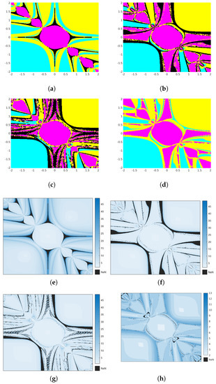
We used a PC with Intel Core i7 processor running Ubuntu 22.4.1 LTS. The programs were executed using MATLAB programming language with version code R2022b.

4. Conclusions

Traub’s method (also known as Arithmetic-Mean Newton’s Method and Weerakoon and Fernando method) and its two extensions were studied in this paper using assumptions on the derivatives of the operator up to the order two. The theoretical parameters are verified using examples. The dynamics of the methods are also included in this study.

References

- Magrenán, A.A.; Argyros, I.K. A Contemporary Study of Iterative Methods: Convergence. Dynamics and Applications; Academic Press: London, UK, 2018. [Google Scholar]
- Ortega, J.M.; Rheinboldt, W.C. Iterative Solution of Nonlinear Equations in Several Variables; Computer Science and Applied Mathematics; Academic Press: New York, NY, USA, 1970; ISBN 978-0-12-528550-6. [Google Scholar]
- Behla, R.; Arora, H. CMMSE: A novel scheme having seventh-order convergence for nonlinear systems. J. Comput. Appl. Math. 2022, 404, 113301. [Google Scholar] [CrossRef]
- Shakhno, S.M. On an iterative algorithm with superquadratic convergence for solving nonlinear operator equations. J. Comput. Appl. Math. 2009, 231, 222–235. [Google Scholar] [CrossRef]
- Traub, J.F. Iterative Methods for the Solution of Equations; Chelsea Publishing: New York, NY, USA, 1982; ISBN 978-0-8284-0312-2. [Google Scholar]
- Petković, M. Multipoint Methods for Solving Nonlinear Equations; Elsevier/Academic Press: Amsterdam, The Netherlands, 2013. [Google Scholar]
- Özban, A.Y. Some new variants of Newton’s method. Appl. Math. Lett. 2004, 17, 677–682. [Google Scholar] [CrossRef]
- Petković, L.D.; Petković, M.S. A note on some recent methods for solving nonlinear equations. Appl. Math. Comput. 2007, 185, 368–374. [Google Scholar] [CrossRef]
- Weerakoon, S.; Fernando, T.G.I. A variant of Newton’s method with accelerated third-order convergence. Appl. Math. Lett. 2000, 13, 87–93. [Google Scholar] [CrossRef]
- Frontini, M.; Sormani, E. Some variant of Newton’s method with third-order convergence. Appl. Math. Comput. 2003, 140, 419–426. [Google Scholar] [CrossRef]
- Cordero, A.; Hueso, J.L.; Martínez, E.; Torregrosa, J.R. Increasing the convergence order of an iterative method for nonlinear systems. Appl. Math. Lett. 2012, 25, 2369–2374. [Google Scholar] [CrossRef]
- Sharma, D.; Parhi, S.K. On the local convergence of modified Weerakoon’s method in Banach spaces. J. Anal. 2020, 28, 867–877. [Google Scholar] [CrossRef]
- Argyros, I.K.; Cho, Y.J.; George, S. Local convergence for some third-order iterative methods under weak conditions. J. Korean Math. Soc. 2016, 53, 781–793. [Google Scholar] [CrossRef]
- Nishani, H.P.S.; Weerakoon, S.; Fernando, T.G.I.; Liyanage, M. Weerakoon-Fernando Method with accelerated third-order convergence for systems of nonlinear equations. IJMMNO 2018, 8, 287. [Google Scholar] [CrossRef]
- Parhi, S.K.; Gupta, D.K. A sixth order method for nonlinear equations. Appl. Math. Comput. 2008, 203, 50–55. [Google Scholar] [CrossRef]
- George, S.; Sadan, A.R.; Jidesh, P.; Argyros, I.K. On the Order of Convergence of Noor-Waseem Method. Mathematics 2022, 10, 4544. [Google Scholar] [CrossRef]
- Beyer, W.A.; Ebanks, B.R.; Qualls, C.R. Convergence rates and convergence-order profiles for sequences. Acta Appl. Math. 1990, 20, 267–284. [Google Scholar] [CrossRef]
- Petković, M.S.; Neta, B.; Petković, L.D.; Džunić, J. Multipoint methods for solving nonlinear equations: A survey. Appl. Math. Comput. 2014, 226, 635–660. [Google Scholar] [CrossRef]
- Ezquerro, J.A.; Hernández, M.A. On the R-order of convergence of Newton’s method under mild differentiability conditions. J. Comput. Appl. Math. 2006, 197, 53–61. [Google Scholar] [CrossRef]
- Potra, F.A.; Pták, V. Nondiscrete Induction and Iterative Processes; Pitman: New York, NY, USA, 1984. [Google Scholar]
- Cordero, A.; Torregrosa, J.R. Variants of Newton’s Method using fifth-order quadrature formulas. Appl. Math. Comput. 2007, 190, 686–698. [Google Scholar] [CrossRef]
- Argyros, I.K. The Theory and Applications of Iteration Methods, 2nd ed.; Engineering Series; CRC Press: Boca Raton, FL, USA; Taylor and Francis Group: Abingdon, UK, 2022. [Google Scholar]
- Chicharro, F.I.; Cordero, A.; Torregrosa, J.R. Drawing Dynamical and Parameters Planes of Iterative Families and Methods. Sci. World J. 2013, 2013, e780153. [Google Scholar] [CrossRef] [PubMed]
- Ardelean, G. A comparison between iterative methods by using the basins of attraction. Appl. Math. Comput. 2011, 218, 88–95. [Google Scholar] [CrossRef]
Disclaimer/Publisher’s Note: The statements, opinions and data contained in all publications are solely those of the individual author(s) and contributor(s) and not of MDPI and/or the editor(s). MDPI and/or the editor(s) disclaim responsibility for any injury to people or property resulting from any ideas, methods, instructions or products referred to in the content. |
© 2023 by the authors. Licensee MDPI, Basel, Switzerland. This article is an open access article distributed under the terms and conditions of the Creative Commons Attribution (CC BY) license (https://creativecommons.org/licenses/by/4.0/).