Numerical Treatment of Multi-Term Fractional Differential Equations via New Kind of Generalized Chebyshev Polynomials

Abstract

The main aim of this paper is to introduce a new class of orthogonal polynomials that generalizes the class of Chebyshev polynomials of the first kind. Some basic properties of the generalized Chebyshev polynomials and their shifted ones are established. Additionally, some new formulas concerned with these generalized polynomials are established. These generalized orthogonal polynomials are employed to treat the multi-term linear fractional differential equations (FDEs) that include some specific problems that arise in many applications. The basic idea behind the derivation of our proposed algorithm is built on utilizing a new power form representation of the shifted generalized Chebyshev polynomials along with the application of the spectral Galerkin method to transform the FDE governed by its initial conditions into a system of linear equations that can be efficiently solved via a suitable numerical solver. Some illustrative examples accompanied by comparisons with some other methods are presented to show that the presented algorithm is useful and effective.

1. Introduction

Numerous scientific and engineering disciplines rely heavily on fractional calculus, including economics [1], viscoelasticity [2], and hydrology [3]. Many phenomena that arise in the different fields of applied sciences can be modeled by fractional differential equations (FDEs), so studies regarding these types of equations are important. Because explicit analytic solutions are often not obtainable for these equations, approximate techniques based on numerical algorithms are often required. For examples of articles concerned with different numerical methods for solving FDEs, see, for example, [4,5,6,7,8,9]. Different multi-term FDEs are used to model many models that arise in many domains, such as rheology and mechanical models; for example, see [10]. A number of articles focus on dealing with these FDEs because of how crucial they are. Spectral methods were heavily relied upon in order to solve these problems. For example, the authors in [11] established an operational matrix of fractional derivatives of Fibonacci polynomials in the Caputo sense, and they employed them to treat some types of muti-type FDEs. Some other techniques were utilized to treat multi-term FDEs. For example, in [12], the authors followed a wavelet approach to treat certain types of multi-term FDEs. Two numerical algorithms were utilized in [13] to treat multi-term fractional diffusion-wave equations. In [14], the authors followed certain difference schemes for treating the time multi-term fractional wave equation.

It is possible to categorize the numerical methods used for differential equations into local and global categories. In contrast to the spectral method, which takes a more global approach, the finite-difference and finite-element approaches are founded on locally relevant arguments. In reality, problems with complex geometries are particularly well-suited to finite-element methods, while spectral methods can offer greater accuracy. There are three main types of spectral methods used to solve the various integral and differential equations that were considered. For the tau and Galerkin spectral methods, we select two sets of basis functions, respectively referred to as “trial” and “test” functions. When employing the Galerkin approach, we select trial functions so that all of them verify the underlying conditions. In this case, the trial functions are the same as the test functions. (see, for example, [15,16,17]). In contrast, the tau method allows for flexibility in selecting both of the basis functions. Based on this comparison, the tau method appears to be more flexible than the Galerkin approach (see, for example, [18,19]). Of all the spectral approaches, the collocation approach seems to be the most used for any differential equation. For example, it is used to solve the fourth-order BVPs (see, [20]). The author in [21] applied two schemes based on the Fibonacci operational matrix to treat the nonlinear fractional Klein–Gordon equation. The author in [22] employed the fractional-order shifted Legendre collocation method for a type of fractional Fredholm integro-differential equations. Another type of FDEs is treated using the implicit wavelet collocation method in [23]).

Chebyshev polynomials were defined nearly a century ago by the Russian mathematician “Chebyshev”. However, Lanczos, a pioneer in the field of numerical mathematics, rediscovered their importance for practical computation some thirty years ago. The introduction of the digital computer emphasized this advancement even more. Of the various sets of orthogonal polynomials, the Chebyshev polynomials have a long history because they have a trigonometric representation. These polynomials are regarded as special Jacobi polynomials as well. There are four distinct Chebyshev polynomials in Jacobi polynomials. All of these kinds can be represented trigonometrically, which is advantageous for using them in various applications. They play a great part in numerical analysis and approximation theory. The first and second kinds are most frequently used in treating different types of differential equations (see, for instance, [24]). The third and fourth kinds, in addition, were also used in a variety of applications. They were employed in [25] to treat the non-linear Lane–Emden-type equations. In addition, they were utilized in [26] to obtain a numerical solution for multi-term variable order FEDs using the shifted third-kind Chebyshev polynomials. Recently, the two types of Chebyshev polynomials, called Chebyshev polynomials of the fifth and sixth kinds, were utilized to treat several types of differential equations. For instance, the fifth-kind Chebyshev polynomials were employed in [27] to treat a multi-term variable-order time-fractional diffusion-wave equation. In addition, Abd-Elhameed in [28] derived new expressions for the high-order derivatives of the sixth-kind Chebyshev polynomials and utilized them to treat the non-linear one-dimensional Burgers’ equation.

Numerous theoretical and practical investigations concerning different generalized and modified polynomials have been carried out. Regarding the modified and generalized polynomials of Chebyshev polynomials, the authors in [29] introduced certain generalized shifted Chebyshev polynomials. In addition, they employed them to handle fractional optimal control problems. A type of multi-dimensional Chebyshev polynomials is introduced in [30]. Another type of generalized second-kind Chebyshev polynomials is introduced in [31]. The authors in [32] established some new formulas for a class of polynomials that generalizes the third-kind Chebyshev polynomials class. In addition, they employed this class of polynomials to treat certain types of even-order BVPs. The authors in [33,34] handled some BVPs and IVP using the Chebyshev polynomials’ first derivative.

This paper is dedicated to introducing a type of orthogonal generalized Chebyshev polynomials of the first kind. Their shifted polynomials are also introduced. Aiming to employ these polynomials from a practical point of view, some fundamental properties of the shifted polynomials will be established. More precisely, the orthogonality relation, power form and inversion formulas of these polynomials will be also found in simple forms that are free of any hypergeometric forms. This type of polynomial will be employed for treating multi-term FDEs.

We believe that the following two issues account for the novelty of the contribution in this paper:

• The theoretical results for the developed type of generalized Chebyshev polynomials are novel.
• The employment of these polynomials from a numerical point of view is also new.

The above two reasons, of course, motivate us to investigate this kind of generalized Chebyshev polynomial both theoretically and practically.

This paper has the following structure: The next section presents some preliminary information involving an overview of certain polynomials that involve five parameters along with some properties of fractional calculus. A new type of generalized polynomials of the first kind and their shifted ones is introduced in Section 3. The proposed numerical algorithm for treating the multi-term FDEs is proposed in Section 4. Numerical experiments are displayed in Section 5 to validate the efficiency and applicability of our proposed algorithm. Finally, the conclusion is presented in Section 6.

2. Preliminaries and Some Fundamental Formulas

This section is confined to presenting an overview of a certain generalized polynomial sequence that generalizes some well-known classes of orthogonal polynomials. Furthermore, some fundamental properties of fractional calculus are presented.

2.1. An Overview on Certain Orthogonal Polynomials of Five Parameters

In his interesting PhD thesis [35], Masjed-Jamei investigated the polynomial solution of the differential equation

$$\left(a{x}^2+bx+c\right){\varphi }_i^{″}\left(x\right)+(dx+e){\varphi }_i^{\prime }\left(x\right)-i\left((i-1)a+d\right){\varphi }_i\left(x\right)=0.$$

(1)

The main advantage of investigating the polynomials that satisfy the second-order recurrence relation (1) is that they generalize some well-known classical polynomials. It was shown in [35] that the monic polynomials solution of (1) is given by the following explicit formula:

$${\displaystyle {\varphi }_i\left(x\right)={\varphi }_i^{a,b,c,d,e}\left(x\right)=\sum _{k=0}^i{A}_{k,i}(a,b,c,d,e)x^k,}$$

(2)

where the coefficients $A_{k,i}(a,b,c,d,e)$ are explicitly given by

$$\begin{array}{cc}\hfill A_{k,i}(a,b,c,d,e)=& \left(\genfrac{}{}{0pt}{}{i}{k}\right){\left(\frac{2a}{b+\sqrt{b^2-4ac}}\right)}^{k-i}\times \hfill \\ \hfill & {}_2{F}_1\left.\left(\begin{array}{c}{\displaystyle k-i,\frac{2ae-bd}{2a\sqrt{b^2-4ac}}+1-\frac{d}{2a}-i}\\ {\displaystyle 2-\frac{d}{a}-2i}\end{array}\right|\frac{2\sqrt{b^2-4ac}}{b+\sqrt{b^2-4ac}}\right).\hfill \end{array}$$

(3)

Note that the coefficients $\left(\genfrac{}{}{0pt}{}{i}{k}\right)$ are the well-known binomial coefficients. In addition, the ${}_2{F}_1$ that appears in (3) is the hypergeometric function that is a special case of the following generalized hypergeometric function ${}_r{F}_s\left.\left(\begin{array}{c}{\alpha }_1,{\alpha }_2,\dots ,{\alpha }_r\\ {\beta }_1,{\beta }_2,\dots ,{\beta }_s\end{array}\right|x\right)$ defined as [36]:

$${\displaystyle {}_r{F}_s\left.\left(\begin{array}{c}{\alpha }_1,{\alpha }_2,\dots ,{\alpha }_r\\ {\beta }_1,{\beta }_2,\dots ,d_s\end{array}\right|x\right)=\sum _{\ell =0}^{\infty }\frac{{\left({\alpha }_1\right)}_{\ell }{\left({\alpha }_2\right)}_{\ell }\dots {\left({\alpha }_r\right)}_{\ell }}{{\left({\beta }_1\right)}_{\ell }{\left({\beta }_2\right)}_{\ell }\dots {\left({\beta }_s\right)}_{\ell }}\frac{x^{\ell }}{\ell !},}$$

where r and s are non-negative integers, and no ${\beta }_i,1\le i\le s$ is zero or a negative integer, and the symbol ${\left(z\right)}_{\ell }$ denotes the Pochhammer symbol.

The author in [35] commented that many general properties of the polynomials in (2) whose power form representation is given in (2) were presented in the famous book of Nikiforov and Uvarov [37]. For example, the Rodrigues formula for ${\varphi }_i^{a,b,c,d,e}\left(x\right)$ is given by

$${\displaystyle {\varphi }_i^{a,b,c,d,e}\left(x\right)=\frac{1}{\left(\frac{d}{a}+i-1\right)a^i{w}^{a,b,c,d,e}\left(x\right)}{D}^i\left\{{(a{x}^2+bx+c)}^i{w}^{a,b,c,d,e}\left(x\right)\right\},}$$

(4)

where $w^{a,b,c,d,e}\left(x\right)$ is given by

$${\displaystyle w^{a,b,c,d,e}\left(x\right)=exp\left({\displaystyle \int \frac{(d-2a)x+(e-b)}{a{x}^2+bx+c}dx}\right).}$$

It was shown in [35] that the polynomials ${\left\{{\varphi }_i^{a,b,c,d,e}\left(x\right)\right\}}_{i\ge 0}$ are orthogonal for suitable choices of the parameters $a,b,c,d$ and e on the interval $(L,U)$ where L and U are the zeros of the second-order equation: $a{x}^2+bx+c=0$. It was also shown that the following important identity is valid:

$${\displaystyle {\int }_L^U{w}^{a,b,c,d,e}\left(x\right){\left({\varphi }_i^{a,b,c,d,e}\left(x\right)\right)}^{2}dx=\frac{{(-1)}^{i}i!}{{\left(\frac{d}{a}+i-1\right)}_i{a}^i}{\int }_L^U{\left(a{x}^2+bx+c\right)}^{i}exp\left({\displaystyle \int \frac{(d-2a)x+(e-b)}{a{x}^2+bx+c}dx}\right)dx.}$$

(5)

Remark 1.

It is worth noting here that the presence of five parameters in the polynomials ${\varphi }_i^{a,b,c,d,e}\left(x\right)$ implies that several sequences of orthogonal polynomials involving the classical Jacobi and Laguerre polynomials are special ones of the generalized polynomials. This, of course, shows the importance of investigating such polynomials and their special classes.

Remark 2.

It is important to note that the formulas involving the five-parameter polynomials ${\varphi }_i^{a,b,c,d,e}\left(x\right)$ are challenging to apply in practice. Consequently, we will limit ourselves to selecting appropriate parameters that allow us to derive some fundamental properties of these polynomials and use them to solve several types of differential equations.

2.2. Some Fundamentals of Fractional Calculus

Some elementary characteristics of certain fractional derivative operators are shown here.

2.2.1. Riemann-Liouville Definition

Definition 1.

The following is the definition of the Riemann–Liouville fractional integral operator ${\mathfrak{I}}_x^{\upsilon }$ of order $\upsilon >0$

$${\displaystyle {\mathfrak{I}}_x^{\upsilon }\mathcal{Z}\left(x\right)=\frac{1}{\mathsf{\Gamma }\left(\upsilon \right)}{\int }_0^x\frac{\mathcal{Z}\left(\tau \right)}{{(x-\tau )}^{1-\upsilon }}d\tau ,}$$

in which the well-known Gamma function is represented by $\mathsf{\Gamma }(.)$.

Definition 2.

The Riemann–Liouville fractional derivative operator ${\mathfrak{D}}_x^{\upsilon }$ of order $\upsilon >0$ is defined as

$${\mathfrak{D}}_x^{\upsilon }\mathcal{Z}\left(x\right)=\frac{d^n}{d{x}^n}{\mathfrak{I}}_x^{n-\upsilon }\mathcal{Z}\left(x\right),n-1\le \upsilon <n,n\in \mathbb{N}.$$

2.2.2. Caputo Definition

Definition 3.

The Caputo fractional derivative operator ${\mathcal{D}}_x^{\upsilon }$ of order $\upsilon >0$ is defined as

$${\mathcal{D}}_x^{\upsilon }\mathcal{Z}\left(x\right)=\frac{1}{\mathsf{\Gamma }(\lceil \upsilon \rceil -\upsilon )}{\int }_0^x\frac{{\mathcal{Z}}^{(\lceil \upsilon \rceil )}\left(\tau \right)}{{(x-\tau )}^{\upsilon +1-\lceil \upsilon \rceil }}d\tau ,x>0,$$

where $\lceil .\rceil$ denotes the well-known ceiling function.

Property 1.

The basic properties of the Caputo fractional integral ${\mathcal{I}}_x^{\upsilon }$ and derivative ${\mathcal{D}}_x^{\upsilon }$ operators of order $\upsilon >0$ are

$${\mathcal{I}}_x^{\upsilon }{x}^n=\frac{\mathsf{\Gamma }(n+1)}{\mathsf{\Gamma }(n+1+\upsilon )}{x}^{n+\upsilon },n\in \mathbb{N},n\ge \lceil \upsilon \rceil ,$$

and

$${\mathcal{D}}_x^{\upsilon }{x}^n=\frac{\mathsf{\Gamma }(n+1)}{\mathsf{\Gamma }(n+1-\upsilon )}{x}^{n-\upsilon },n\in \mathbb{N},n\ge \lceil \upsilon \rceil .$$

(6)

For more details about fractional calculus, one can consult [38,39].

3. A Kind of Generalized First-Kind Chebyshev Polynomials

This section is confined to introducing a new class of polynomials that generalizes the class of Chebyshev polynomials of the first kind. In addition, we will present some fundamental properties of these polynomials. Furthermore, the shifted generalized Chebyshev polynomials will be introduced, and some of their fundamental properties will be developed.

3.1. Introducing Generalized Chebyshev Polynomials of the First Kind

In this section, we will extract a generalized class of Chebyshev polynomials. This class is a special class of the class of polynomials ${\varphi }_i^{a,b,c,d,e}\left(x\right)$ in (2). For this purpose, we make the following choices:

$$a=-1,c=b+1,d=-1,e=0.$$

(7)

Thus, we have only a free parameter b. Let us denote the resulting polynomials by $T_i^b\left(x\right)$. That is

$${\displaystyle T_i^b\left(x\right)=\sum _{k=0}^i{A}_{k,i}(-1,b,b+1,-1,0)x^k.}$$

It can be seen that the polynomials $T_i^b\left(x\right)$ are orthogonal on $[-1,b+1]$ with respect to the following weight function $w\left(x\right)$:

$$w\left(x\right)={(b-x+1)}^{-\frac{1}{b+2}}{(1+x)}^{-\frac{b+1}{b+2}}.$$

(8)

From the Rodrigues formula in (4) for the polynomials ${\varphi }_i^{a,b,c,d,e}\left(x\right)$, it can be shown that the Rodrigues formula for the polynomials $T_i^b\left(x\right)$ is given by

$${\displaystyle T_i^b\left(x\right)=\frac{2{(-1)}^{i}i!}{\left(2i\right)!w\left(x\right)}{D}^i\left\{{(b-x+1)}^i{(1+x)}^{i}w\left(x\right)\right\},i\ge 1.}$$

(9)

We comment here that we have two main reasons for selecting the five parameters as in (7):

• These choices will lead to reducing the generalized polynomials of five parameters that are given in (2) into polynomials involving one parameter that generalizes the Chebyshev polynomials of the first kind. Thus, this generalization is a new generalization of the first kind of Chebyshev polynomials that was not investigated before from both theatrical and practical points of view.
• This choice will lead to a simplified power form and inversion formulas for the shifted generalized polynomials on $[0,1]$. We will show that these formulas do not involve any hypergeometric functions. These formulas will be of fundamental importance in the sequel.

Now, we are going to find the orthogonality relation to the polynomials $T_i^b\left(x\right)$. First, the following lemma is needed.

Lemma 1.

For every positive integer n and every non-negative real number b, the following integral formula holds:

$$\underset{-1}{\overset{b+1}{\int }}{\left(1+b+bx-x^2\right)}^{n}w\left(x\right)dx=\frac{{(b+2)}^{2n}\mathsf{\Gamma }\left(\frac{1}{b+2}+n\right)\mathsf{\Gamma }\left(\frac{b+1}{b+2}+n\right)}{\left(2n\right)!}.$$

Proof. 

In order to make the integral easier to compute, we replace x by $\left((b+2)x-1\right)$, that is, we have the following formula:

$${\int }_{-1}^{b+1}{\left(1+b+bx-x^2\right)}^{n}w\left(x\right)dx={(b+2)}^{2n}{\int }_0^1{(1-x)}^{-\frac{1}{b+2}+n}{x}^{-1+\frac{1}{b+2}+n}dx.$$

It is not difficult to show that the following identity holds:

$${\int }_0^1{(1-x)}^{n-\frac{1}{b+2}}{x}^{n-\frac{b+1}{b+2}}dx=\frac{\mathsf{\Gamma }\left(\frac{1}{b+2}+n\right)\mathsf{\Gamma }\left(\frac{b+1}{b+2}+n\right)}{\left(2n\right)!},$$

and this accordingly leads to the following identity:

$${\int }_{-1}^{b+1}{\left(1+b+bx-x^2\right)}^{n}w\left(x\right)dx=\frac{{(b+2)}^{2n}\mathsf{\Gamma }\left(\frac{1}{b+2}+n\right)\mathsf{\Gamma }\left(\frac{b+1}{b+2}+n\right)}{\left(2n\right)!}.$$

Lemma 1 is now proved. □

Now, we are able to state and prove the following relation of $T_i^b\left(x\right).$

Theorem 1.

For every positive integer i and every non-negative real number b, the following integral formula holds:

$${\int }_{-1}^{b+1}{\left(T_i^b\left(x\right)\right)}^{2}w\left(x\right)dx=\frac{2^{1-4i}{(b+2)}^{2i}\pi \mathsf{\Gamma }\left(\frac{1}{b+2}+i\right)\mathsf{\Gamma }\left(\frac{b+1}{b+2}+i\right)}{{\left(\mathsf{\Gamma }\left(i+\frac{1}{2}\right)\right)}^2},$$

(10)

where the weight function $w\left(x\right)$ is given by (8).

Proof. 

The proof of Identity (10) is based on making use of Formula (5). More precisely, if we substitute by $a=-1,c=b+1,d=-1,e=0$, then we obtain

$${\int }_{-1}^{b+1}{\left(T_i^b\left(x\right)\right)}^{2}w\left(x\right)dx=\frac{2{(i!)}^2}{\left(2i\right)!}{\int }_{-1}^{b+1}{\left(1+b+bx-x^2\right)}^{i}w\left(x\right)dx.$$

The direct application to Lemma 1 yields Formula (10). □

3.2. Shifted Generalized Chebyshev Polynomials

In many practical problems and applications, it is required to define and employ the shifted polynomials on the interval $[0,1]$. We define the shifted polynomials $S{T}_i^b\left(x\right)$ on $[0,1]$ as

$$S{T}_i^b\left(x\right)=T_i^b\left((b+2)x-1\right).$$

(11)

The Rodrigues formula for the generalized Chebyshev polynomials $T_i^b\left(x\right)$ in (9) can be easily transformed to give the counterpart for the shifted generalized Chebyshev polynomials that are defined in (11). In fact, the polynomials $S{T}_i^b$(x) may be generated using the following Rodrigues formula:

$${\displaystyle S{T}_i^b\left(x\right)=\frac{2{(-1)}^{i}i!{(b+2)}^i}{\left(2i\right)!\tilde{w}\left(x\right)}{D}^i\left\{{(1-x)}^i{x}^i\tilde{w}\left(x\right)\right\},i\ge 1,}$$

where $\tilde{w}\left(x\right)$ is given by:

$$\tilde{w}\left(x\right)=\frac{1}{b+2}{x}^{\frac{1}{b+2}-1}{(1-x)}^{-\frac{1}{b+2}}.$$

For our subsequent purposes, it is very useful to establish some fundamental properties of the shifted generalized Chebyshev polynomials $S{T}_i^b\left(x\right)$. The following two theorems display the power form representation and inversion formula to the polynomials $S{T}_i^b\left(x\right)$.

Theorem 2.

For every non-negative integer i, the polynomials $S{T}_i^b\left(x\right)$ can be represented explicitly in the following form:

$$S{T}_i^b\left(x\right)={(b+2)}^i\sum _{k=0}^i\frac{{(-1)}^k\left(\genfrac{}{}{0pt}{}{i}{k}\right){\left(\frac{1}{b+2}+i-k\right)}_k}{{(2i-k)}_k}{x}^{i-k}.$$

(12)

Proof. 

If we substitute by the following choices: $a=-1,c=b+1,d=-1,e=0$ in the general Formula (2), then it reduces to the following formula:

$$T_i^b\left(x\right)=\sum _{k=0}^i{G}_{k,i}{x}^k,$$

(13)

where $G_{k,i}=A\left(-1,b,b+1,-1,0\right)$ are given by

$$G_{k,i}=2^{k-i}{\left({\displaystyle \frac{-1}{2(b+1)}}\right)}^{k-i}\left(\genfrac{}{}{0pt}{}{i}{k}\right){}_2{F}_1\left.\left(\begin{array}{c}k-i,\frac{1}{b+2}-i\\ 1-2i\end{array}\right|\frac{b+2}{b+1}\right).$$

The power form representation of the shifted polynomials $S{T}_i^b\left(x\right)$ on $[0,1]$ can be obtained from relation (13) by replacing x by $\left((b+2)x-1\right)$. Therefore, we can write the following formula:

$$S{T}_i^b\left(x\right)=\sum _{k=0}^i{G}_{k,i}{((b+2)x-1)}^k,$$

which can be written alternatively in the form:

$$S{T}_i^b\left(x\right)=\sum _{k=0}^i{F}_{k,i}{((b+2)x-1)}^{i-k},$$

(14)

where $F_{k,i}$ are given as follows:

$$F_{k,i}={(-1)}^k{(b+1)}^k\left(\genfrac{}{}{0pt}{}{i}{i-k}\right){}_2{F}_1\left.\left(\begin{array}{c}-k,\frac{1}{b+2}-i\\ 1-2i\end{array}\right|\frac{b+2}{b+1}\right).$$

The binomial theorem enables one to write Formula (14) in the following form:

$$S{T}_i^b\left(x\right)=\sum _{k=0}^i{F}_{k,i}\sum _{\ell =0}^{i-k}{B}_{\ell ,k,i}{x}^{\ell },$$

(15)

where the coefficients $B_{\ell ,k,i}$ are given as:

$$B_{\ell ,k,i}={(-1)}^{i-k-\ell }{(b+2)}^{\ell }\left(\genfrac{}{}{0pt}{}{i-k}{\ell }\right).$$

Performing some manipulations on (15) turns it into the following form:

$$S{T}_i^b\left(x\right)=\sum _{k=0}^i{H}_{k,i}{x}^{i-k},$$

where the coefficients $H_{k,i}$ are given explicitly by

$$H_{k,i}={(b+2)}^{i-k}\sum _{\ell =0}^k{(-1)}^k{(b+1)}^{\ell }\left(\genfrac{}{}{0pt}{}{i}{i-\ell }\right)\left(\genfrac{}{}{0pt}{}{i-\ell }{i-k}\right){}_2{F}_1\left.\left(\begin{array}{c}-\ell ,\frac{1}{b+2}-i\\ 1-2i\end{array}\right|\frac{b+2}{b+1}\right).$$

(16)

Although the hypergeometric form in (16) cannot be summed except for specific values of the parameter b, the coefficients $H_{k,i}$ can be reduced for all values of b using the celebrated algorithm of Zeilberger [40]. In fact, the employment of this algorithm shows that the following recurrence relation of order one can be obtained:

$$H_{k+1,i}-\frac{(k-i)(1+b+2k+bk-(b+2\left)i\right)}{(b+2)(1+k)(1+k-2i)}{H}_{k,i}=0,H_{0,i}={(b+2)}^i.$$

Given that the last recurrence relation is of order one, its solution can be provided immediately in the form:

$$H_{k,i}=\frac{{(-1)}^k\left(\genfrac{}{}{0pt}{}{i}{k}\right){(b+2)}^i{\left(\frac{1}{b+2}+i-k\right)}_k}{{(2i-k)}_k}.$$

Therefore, Formula (12) is now proved. □

Now, the integral formula that corresponds to Formula (10) regarding the shifted polynomials $S{T}_i^b\left(x\right)$ will be stated and proved in the following corollary.

Corollary 1.

For every non-negative integer i and every non-negative real number b, the following integral formula is valid:

$${\int }_0^1{\left(S{T}_i^b\left(x\right)\right)}^2\tilde{w}\left(x\right)dx=\frac{2^{1-4i}{(b+2)}^{2i-1}\pi \mathsf{\Gamma }\left(\frac{1}{b+2}+i\right)\mathsf{\Gamma }\left(1-\frac{1}{b+2}+i\right)}{{\left(\mathsf{\Gamma }\left(i+\frac{1}{2}\right)\right)}^2}.$$

(17)

Proof. 

A direct consequence of relation (10). □

We will now present and demonstrate a significant theorem that illustrates the inversion formula of the shifted polynomials $S{T}_i^b\left(x\right)$. The following lemma is necessary first.

Lemma 2.

For all non-negative integers r and j with $r\ge j$, the following identity applies:

$$\begin{array}{c}\hfill {\displaystyle \sum _{m=0}^{r-j}\frac{{(-1)}^m\left(\genfrac{}{}{0pt}{}{r-j}{m}\right)\mathsf{\Gamma }\left(\frac{1}{b+2}-j-m+2r\right){\left(\frac{1}{b+2}-j-m+r\right)}_m}{(2r-j-m)!{(2r-2j-m)}_m}=\frac{{\theta }_{r-j}\sqrt{\pi }r!\mathsf{\Gamma }\left(\frac{1}{b+2}+r\right)\mathsf{\Gamma }\left(\frac{b+1}{b+2}-j+r\right)}{2^{2r-2j-1}\mathsf{\Gamma }\left(\frac{b+1}{b+2}\right)j!(2r-j)!\mathsf{\Gamma }\left(\frac{1}{2}-j+r\right)},}\end{array}$$

(18)

where ${\theta }_{\ell }$ is defined as

$${\theta }_{\ell }=\left\{\begin{array}{cc}\frac{1}{2},\hfill & \ell =0,\hfill \\ 1,\hfill & \ell >0.\hfill \end{array}\right.$$

(19)

Proof. 

Setting $\ell =r-j\ge 0$, then to prove Identity (18), it is enough to prove the following identity:

$$\begin{array}{c}\hfill \sum _{m=0}^{\ell }\frac{{(-1)}^m\left(\genfrac{}{}{0pt}{}{\ell }{m}\right)\mathsf{\Gamma }\left(\frac{1}{b+2}+j+2\ell -m\right){\left(\frac{1}{b+2}+\ell -m\right)}_m}{(j+2\ell -m)!{(2\ell -m)}_m}=\frac{\sqrt{\pi }{\theta }_{\ell }\mathsf{\Gamma }\left(\frac{b+1}{b+2}+\ell \right)(j+\ell )!\mathsf{\Gamma }\left(\frac{1}{b+2}+j+\ell \right)}{2^{2\ell -1}j!(j+2\ell )!\mathsf{\Gamma }\left(\frac{b+1}{b+2}\right)\mathsf{\Gamma }\left(\frac{1}{2}+\ell \right)}.\end{array}$$

For this purpose, set

$$S_{\ell ,j}=\sum _{m=0}^{\ell }\frac{{(-1)}^m\left(\genfrac{}{}{0pt}{}{\ell }{m}\right)\mathsf{\Gamma }\left(\frac{1}{b+2}+j+2\ell -m\right){\left(\frac{1}{b+2}+\ell -m\right)}_m}{(j+2\ell -m)!{(2\ell -m)}_m}.$$

The utilization of Zeilberger’s algorithm again [40] demonstrates that the following first-order recurrence relation is satisfied by $S_{\ell ,j}$:

$$\begin{array}{cc}\hfill & 2{(b+2)}^2(1+j+2\ell )(2+j+2\ell )(1+2\ell ){\theta }_{\ell }{S}_{\ell +1,j}\hfill \\ \hfill & -(1+j+\ell )(1+b+(b+2)\ell )(1+(b+2)j+(b+2)\ell )S_{\ell ,j}=0,\hfill \end{array}$$

(20)

with the initial value

$$S_{0,j}=1,$$

Immediately, we may solve the recurrence relation (20) to obtain

$$S_{\ell ,j}=\frac{\sqrt{\pi }{\theta }_{\ell }\mathsf{\Gamma }\left(\frac{b+1}{b+2}+\ell \right)(j+\ell )!\mathsf{\Gamma }\left(\frac{1}{b+2}+j+\ell \right)}{2^{2\ell -1}j!(j+2\ell )!\mathsf{\Gamma }\left(\frac{b+1}{b+2}\right)\mathsf{\Gamma }\left(\frac{1}{2}+\ell \right)}.$$

This proves Formula (18), and hence completes the proof of Lemma 2. □

Theorem 3.

For every non-negative integer r, the following formula holds:

$$x^r=\sum _{j=0}^r\frac{{(b+2)}^{j-r}{(1+r-j)}_j{\left(\frac{1}{b+2}+r-j\right)}_j}{j!{(2r-2j+1)}_j}S{T}_{r-j}^b\left(x\right).$$

(21)

Proof. 

First, we can write the identity:

$${\displaystyle x^r=\sum _{j=0}^r{A}_{j,r}S{T}_{r-j}^b\left(x\right),}$$

(22)

then to prove Identity (21), we have to find the coefficients $A_{j,r}$.

Now, multiplying both sides of (22) by $S{T}_m^b\left(x\right)\tilde{w}\left(x\right)$ and integrating from 0 to 1, we obtain

$${\displaystyle \sum _{j=0}^r{A}_{j,r}{\int }_0^{1}S{T}_{r-j}^b\left(x\right)S{T}_m^b\left(x\right)\tilde{w}\left(x\right)dx={\int }_0^1{x}^{r}S{T}_m^b\left(x\right)\tilde{w}\left(x\right)dx.}$$

The orthogonality relation of $S{T}_i^b\left(x\right)$ in (17) enables one to determine the coefficients $A_{j,r}$ in the form

$${\displaystyle A_{j,r}=\frac{1}{h_{r-j}{\theta }_{r-j}}{\int }_0^1{x}^{r}S{T}_{r-j}^b\left(x\right)\tilde{w}\left(x\right)dx,}$$

(23)

where ${\theta }_{\ell }$ is as defined in (19).

Now, from the power form representation of $S{T}_i^b\left(x\right)$ in (12), we can write

$${\displaystyle S{T}_i^b\left(x\right)=\sum _{m=0}^i{H}_{m,i}{x}^{i-m},}$$

(24)

where the coefficients $H_{m,i}$ are given by (16).

Inserting Formula (24) into Formula (23), the coefficients $A_{j,r}$ can be written in the form

$${\displaystyle A_{j,r}=\frac{1}{h_{r-j}{\theta }_{r-j}}\sum _{m=0}^{r-j}{H}_{m,r-j}{\int }_0^1{x}^{2r-j-m}\tilde{w}\left(x\right)dx.}$$

(25)

It is not difficult to note the following identity:

$${\int }_0^1{x}^r\tilde{w}\left(x\right)dx=\frac{\mathsf{\Gamma }\left(\frac{b+1}{b+2}\right)\mathsf{\Gamma }\left(\frac{1}{b+2}+r\right)}{(b+2)r!},$$

and consequently, Formula (25) explicitly gives

$$\begin{array}{cc}\hfill A_{j,r}=& \frac{2^{4r-4j-1}{(b+2)}^{j-r}\mathsf{\Gamma }\left(\frac{b+1}{b+2}\right){\left(\mathsf{\Gamma }\left(\frac{1}{2}-j+r\right)\right)}^2}{\pi {\theta }_{r-j}\mathsf{\Gamma }\left(\frac{1}{b+2}-j+r\right)\mathsf{\Gamma }\left(\frac{b+1}{b+2}-j+r\right)}\times \hfill \\ \hfill & \sum _{m=0}^{r-j}\frac{{(-1)}^m\left(\genfrac{}{}{0pt}{}{r-j}{m}\right)\mathsf{\Gamma }\left(\frac{1}{b+2}-j-m+2r\right){\left(\frac{1}{b+2}-j-m+r\right)}_m}{(2r-j-m)!{(2r-2j-m)}_m}.\hfill \end{array}$$

The application of Lemma 2 leads to putting the coefficients $A_{j,r}$ in the following form:

$$A_{j,r}=\frac{{(b+2)}^{j-r}{(1+r-j)}_j{\left(\frac{1}{b+2}+r-j\right)}_j}{j!{(1+2r-2j)}_j}.$$

This finalizes the proof of Theorem 3. □

4. Treating Multi-Term FDEs via the Shifted Polynomials ${\mathit{ST}}_{\mathit{i}}^{\mathit{b}}\left(\mathit{x}\right)$

In this section, we are interested in employing the generalized shifted first-kind Chebyshev–Galerkin method ($GS1KCGM$) to solve the linear FDEs governed by the homogeneous and nonhomogeneous initial conditions.

Before proceeding in developing our proposed algorithm, the following lemma is needed.

Lemma 3.

For every non-negative integer i and for every positive real number μ, the following integral formula holds:

$${\int }_0^1{x}^{\mu }S{T}_i^b\left(x\right)\tilde{w}\left(x\right)dx=\frac{2^{1-2i}\sqrt{\pi }{\theta }_i{(b+2)}^{i-1}\mathsf{\Gamma }(1+\mu )\mathsf{\Gamma }\left(\frac{b+1}{b+2}+i\right)\mathsf{\Gamma }\left(\frac{1}{b+2}+\mu \right)}{\mathsf{\Gamma }\left(\frac{1}{2}+i\right)\mathsf{\Gamma }(1-i+\mu )\mathsf{\Gamma }(1+i+\mu )}.$$

Proof. 

From the inversion Formula (21), the following formula holds for every positive integer r

$$x^r=\sum _{j=0}^r\frac{{(b+2)}^{-j}\left(2j\right)!{(j+1)}_{r-j}{\left(\frac{1}{b+2}+j\right)}_{r-j}}{(r-j)!(r+j)!}S{T}_j^b\left(x\right).$$

However, for any positive real number $\mu$, one can write

$$x^{\mu }=\sum _{j=0}^{\infty }{M}_{j,\mu }S{T}_j^b\left(x\right),$$

where $M_{j,\mu }$ is given by

$$M_{j,\mu }=\frac{{(b+2)}^{-j}\left(2j\right)!{(j+1)}_{\mu -j}{\left(\frac{1}{b+2}+j\right)}_{\mu -j}}{\mathsf{\Gamma }(1-j+\mu )\mathsf{\Gamma }(j+\mu +1)}.$$

Now, we have

$${\displaystyle {\int }_0^1{x}^{\mu }S{T}_i^b\left(x\right)\tilde{w}\left(x\right)dx=\sum _{j=0}^{\infty }{M}_{j,\mu }{\left(S{T}_j^b\left(x\right),S{T}_i^b\left(x\right)\right)}_{\tilde{w}}.}$$

Formula (17) allows one to reduce the last identity into the following form:

$${\displaystyle {\int }_0^1{x}^{\mu }S{T}_i^b\left(x\right)\tilde{w}\left(x\right)dx=M_{i,\mu }{h}_i,}$$

where $h_i$ are given as

$$h_i=\frac{2^{1-4i}{(b+2)}^{2i-1}\pi \mathsf{\Gamma }\left(\frac{1}{b+2}+i\right)\mathsf{\Gamma }\left(1-\frac{1}{b+2}+i\right)}{{\left(\mathsf{\Gamma }\left(i+\frac{1}{2}\right)\right)}^2},$$

and this consequently yields the following identity:

$${\int }_0^1{x}^{\mu }S{T}_i^b\left(x\right)\tilde{w}\left(x\right)dx=\frac{2^{1-2i}\sqrt{\pi }{\theta }_i{(b+2)}^{i-1}\mathsf{\Gamma }(1+\mu )\mathsf{\Gamma }\left(\frac{b+1}{b+2}+i\right)\mathsf{\Gamma }\left(\frac{1}{b+2}+\mu \right)}{\mathsf{\Gamma }\left(\frac{1}{2}+i\right)\mathsf{\Gamma }(1-i+\mu )\mathsf{\Gamma }(1+i+\mu )}.$$

This completes the proof of Lemma 3. □

Our Proposed Galerkin Approach

This section is confined to introducing a Galerkin approach for treating multi-term FDEs. Now consider the following linear FDEs:

$${\mathcal{D}}_x^{{\upsilon }_n}\mathcal{Z}\left(x\right)+\sum _{m=0}^{n-1}{\eta }_m{\mathcal{D}}_x^{{\upsilon }_m}\mathcal{Z}\left(x\right)=g\left(x\right),x\in [0,1],$$

(26)

governed by the following homogeneous initial conditions

$${\mathcal{Z}}^{\left(m\right)}\left(0\right)=0,m=0,1,\dots ,n-1,$$

(27)

where $0\le x\le 1,$ $m-1<{\upsilon }_m\le m,(m=1,2,\cdots ,n)$ and ${\upsilon }_0=0,$ while ${\eta }_m,$ for $m=0,1,2,\dots ,n-1,$ are given constants and $g\left(x\right)$ is a given smooth function on $[0,1],$ while ${\mathcal{D}}_x^{\upsilon }\mathcal{Z}\left(x\right)$ denotes the Caputo fractional derivative of order $\upsilon ,$ with respect to x given in Definition 3.

If we define the following spaces,

$$\begin{array}{cc}\hfill S_N=& \mathrm{span}\{S{T}_0^b\left(x\right),S{T}_1^b\left(x\right),\dots ,S{T}_{N-n}^b\left(x\right)\},\hfill \\ \hfill {\mathsf{\Phi }}_N=& \{\phi \left(x\right)\in S_N:{\phi }^{\left(m\right)}\left(0\right)=0,m=0,1,\dots ,n-1\},\hfill \end{array}$$

then the $GS1KCGM$ approximation to (26) and (27) is to find ${\mathcal{Z}}_N\left(x\right)\in {\mathsf{\Phi }}_N$ such that

$${\left({\mathcal{D}}_x^{{\upsilon }_n}\mathcal{Z}\left(x\right),\phi \left(x\right)\right)}_{\tilde{w}}+\sum _{m=0}^{n-1}{\eta }_m{\left({\mathcal{D}}_x^{{\upsilon }_m}\mathcal{Z}\left(x\right),\phi \left(x\right)\right)}_{\tilde{w}}={(g\left(x\right),\phi \left(x\right))}_{\tilde{w}},\forall \phi \left(x\right)\in {\mathsf{\Phi }}_N,$$

where

$${\displaystyle {\left(\mathcal{Z}\left(x\right),\phi \left(x\right)\right)}_{\tilde{w}}={\int }_0^1\mathcal{Z}\left(x\right)\phi \left(x\right)\tilde{w}\left(x\right)dx.}$$

We construct reasonable basis functions that satisfy the homogeneous initial conditions as

$${\phi }_i\left(x\right)=x^{n}S{T}_i^b\left(x\right),x\in [0,1].$$

(28)

To solve the initial value problem (26) and (27), $\mathcal{Z}\left(x\right)$ can be approximated as

$${\mathcal{Z}}_N\left(x\right)=\sum _{i=0}^{N-n}{c}_i{\phi }_i\left(x\right),x\in [0,1].$$

(29)

Using the approximation in (29), we have

$$\begin{array}{cc}\hfill & \sum _{i=0}^{N-n}{c}_i{\left({\mathcal{D}}_x^{{\upsilon }_n}{\phi }_i\left(x\right),{\phi }_j\left(x\right)\right)}_{\tilde{w}}+\sum _{i=0}^{N-n}{c}_i\sum _{m=0}^{n-1}{\eta }_m{\left({\mathcal{D}}_x^{{\upsilon }_m}{\phi }_i\left(x\right),{\phi }_j\left(x\right)\right)}_{\tilde{w}}={(g\left(x\right),{\phi }_j\left(x\right))}_{\tilde{w}},\hfill \\ \hfill & \forall {\phi }_j\left(x\right)\in {\mathsf{\Phi }}_N.\hfill \end{array}$$

(30)

Let us denote

$$\begin{array}{cccc}\hfill \mathbf{A}& ={\left({\alpha }_{ij}\right)}_{0\le i,j\le N-n},\hfill & \hfill & {\alpha }_{ij}={\left({\mathcal{D}}_x^{{\upsilon }_n}{\phi }_i\left(x\right),{\phi }_j\left(x\right)\right)}_{\tilde{w}},\hfill \\ \hfill {\mathbf{B}}_m& ={\left({\beta }_{ij}^m\right)}_{0\le i,j\le N-n},\hfill & \hfill & {\beta }_{ij}^m={\left({\mathcal{D}}_x^{{\upsilon }_m}{\phi }_i\left(x\right),{\phi }_j\left(x\right)\right)}_{\tilde{w}},0\le m\le n-1,\hfill \\ \hfill \mathbf{G}& ={\left({\gamma }_j\right)}_{0\le j\le N-n},\hfill & \hfill & {\gamma }_j={\left(g\left(x\right),{\phi }_j\left(x\right)\right)}_{\tilde{w}}.\hfill \end{array}$$

Then (30) is equivalent to the following matrix system:

$$\left(\mathbf{A}+\sum _{m=0}^{n-1}{\eta }_m{\mathbf{B}}_m\right)\mathbf{C}=\mathbf{G},$$

(31)

where $\mathbf{C}={\left(c_0,c_1,\dots ,c_{N-n}\right)}^T$ is the unknown vector to be determined. In addition, the nonzero elements of the matrices $\mathbf{A}$ and ${\mathbf{B}}_m(0\le m\le n-1)$ are explicitly provided in the next theorem.

Theorem 4.

Let ${\phi }_i\left(x\right)$ be as selected in (28), and assume that ${\alpha }_{ij}={\left({\mathcal{D}}_x^{{\upsilon }_n}{\phi }_i\left(x\right),{\phi }_j\left(x\right)\right)}_{\tilde{w}}$ and ${\beta }_{ij}^m={\left({\mathcal{D}}_x^{{\upsilon }_m}{\phi }_i\left(x\right),{\phi }_j\left(x\right)\right)}_{\tilde{w}},0\le m\le n-1.$ We have

$${\mathsf{\Phi }}_N=\{{\phi }_0\left(x\right),{\phi }_1\left(x\right),\dots ,{\phi }_{N-n}\left(x\right)\}.$$

Furthermore, the nonzero entries of $\mathit{A}$ and ${\mathit{B}}_m(0\le m\le n-1)$ can be computed by

$${\alpha }_{ij}=\sum _{r=0}^i{\zeta }_{i,j,b,n,{\upsilon }_n},$$

(32)

$${\beta }_{ij}^m=\sum _{r=0}^i{\zeta }_{i,j,b,n,{\upsilon }_m},$$

(33)

where ${\zeta }_{i,j,b,n,\upsilon }$ is given by

$$\begin{array}{cc}\hfill {\zeta }_{i,j,b,n,\upsilon }& =\frac{\sqrt{\pi }{\theta }_j(b+1-(b+2)i)\left(\genfrac{}{}{0pt}{}{i}{r}\right)\mathsf{\Gamma }\left(\frac{b+1}{b+2}+j\right)(i+n-r)!\mathsf{\Gamma }(i+2n-r-\upsilon +1)}{2^{2j-1}{(b+2)}^{2-i-j}\mathsf{\Gamma }\left(j+\frac{1}{2}\right)\mathsf{\Gamma }(i+n-r-\upsilon +1)\mathsf{\Gamma }(i-j+2n-r-\upsilon +1)}\hfill \\ & \times \frac{\mathsf{\Gamma }\left(i+2n-r-\upsilon +\frac{1}{b+2}\right){\left(\frac{b+1}{b+2}-i+1\right)}_{r-1}}{\mathsf{\Gamma }(i+j+2n-r-\upsilon +1){(2i-r)}_r}.\hfill \end{array}$$

Proof. 

The basis functions ${\phi }_i\left(x\right)$ are selected so that each one of its components meets (27). It is also clear that ${\left\{{\phi }_i\left(x\right)\right\}}_{0\le i\le N-n}$ are linearly independent and the dimension of ${\mathsf{\Phi }}_N$ is equal to $(N-n+1)$. Hence,

$${\mathsf{\Phi }}_N=\{{\phi }_0\left(x\right),{\phi }_1\left(x\right),\dots ,{\phi }_{N-n}\left(x\right)\}.$$

Now, we prove (32). Using (28) and Theorem 2, we have

$${\phi }_i\left(x\right)=x^n{(b+2)}^i\sum _{r=0}^i\frac{\left(\genfrac{}{}{0pt}{}{i}{r}\right)\left(1-i-\frac{1}{b+2}\right){\left(1-i+\frac{b+1}{b+2}\right)}_{r-1}}{{(2i-r)}_r}{x}^{i-r},$$

and making use of relation (6) yields

$${\mathcal{D}}_x^{\upsilon }{\phi }_i\left(x\right)={(b+2)}^{i-1}\sum _{r=0}^i\frac{(b+1-(b+2)i)\left(\genfrac{}{}{0pt}{}{i}{r}\right)(i+n-r)!{\left(1-i+\frac{b+1}{b+2}\right)}_{r-1}}{\mathsf{\Gamma }(i+n-r-\upsilon +1){(2i-r)}_r}{x}^{i+n-r-\upsilon },$$

and therefore, we obtain

$$\begin{array}{cc}\hfill {\left({\mathcal{D}}_x^{\upsilon }{\phi }_i\left(x\right),{\phi }_j\left(x\right)\right)}_{\tilde{w}}& =\sum _{r=0}^i\frac{(b+1-(b+2)i)\left(\genfrac{}{}{0pt}{}{i}{r}\right)(i+n-r)!{\left(1-i+\frac{b+1}{b+2}\right)}_{r-1}}{{(b+2)}^{1-i}\mathsf{\Gamma }(i+n-r-\upsilon +1){(2i-r)}_r}{\left(x^{i+n-r-\upsilon },{\phi }_j\left(x\right)\right)}_{\tilde{w}}.\hfill \end{array}$$

If we make use of Lemma 3, then after performing some algebraic computations, we obtain

$${\left({\mathcal{D}}_x^{\upsilon }{\phi }_i\left(x\right),{\phi }_j\left(x\right)\right)}_{\tilde{w}}=\sum _{r=0}^i{\zeta }_{i,j,b,n,\upsilon },$$

where ${\zeta }_{i,j,b,n,\upsilon }$ is given by

$$\begin{array}{cc}\hfill {\zeta }_{i,j,b,n,\upsilon }& =\frac{\sqrt{\pi }{\theta }_j(b+1-(b+2)i)\left(\genfrac{}{}{0pt}{}{i}{r}\right)\mathsf{\Gamma }\left(\frac{b+1}{b+2}+j\right)(i+n-r)!\mathsf{\Gamma }(i+2n-r-\upsilon +1)}{2^{2j-1}{(b+2)}^{2-i-j}\mathsf{\Gamma }\left(j+\frac{1}{2}\right)\mathsf{\Gamma }(i+n-r-\upsilon +1)\mathsf{\Gamma }(i-j+2n-r-\upsilon +1)}\hfill \\ & \times \frac{\mathsf{\Gamma }\left(i+2n-r-\upsilon +\frac{1}{b+2}\right){\left(\frac{b+1}{b+2}-i+1\right)}_{r-1}}{\mathsf{\Gamma }(i+j+2n-r-\upsilon +1){(2i-r)}_r}.\hfill \end{array}$$

Replacing $\upsilon$ by ${\upsilon }_n$ and ${\upsilon }_m$ to prove (32) and (33), respectively, completes the proof.

Finally, using any appropriate numerical algorithm, we solve the linear algebraic system (31) in the unknown coefficients $c_i,i=0,1,\dots ,N-n$. □

Remark 3.

In order to deal with the multi-term linear FDEs (26) directed by non-homogeneous initial conditions, namely,

$${\mathcal{Z}}^{\left(m\right)}\left(0\right)={\delta }_m,m=0,1,\cdots ,n-1,$$

where ${\delta }_m$ are arbitrary constants, $0\le m\le n-1$, the following transformation is used:

$$\tilde{\mathcal{Z}}\left(x\right)=\mathcal{Z}\left(x\right)-\sum _{m=0}^{n-1}\frac{{\delta }_m}{m!}{x}^m,$$

to turn the non-homogeneous conditions into homogeneous ones, and so the same derived algorithm can be utilized.

5. Illustrative Problems and Comparisons

This section is confined to testing our proposed algorithm. For this purpose, we will present four numerical examples accompanied by comparisons with some other techniques in the literature to demonstrate the efficiency and high accuracy of our proposed numerical algorithm.

Example 1.

Consider a composite fractional oscillation equation that immerses in a Newtonian fluid [41,42]:

$${\mathcal{D}}_x^{{\upsilon }_1}\mathcal{Z}\left(x\right)+\mathcal{Z}\left(x\right)=x^4-\frac{1}{2}{x}^3-\frac{3}{\mathsf{\Gamma }(4-{\upsilon }_1)}{x}^{3-{\upsilon }_1}+\frac{24}{\mathsf{\Gamma }(5-{\upsilon }_1)}{x}^{4-{\upsilon }_1},0<{\upsilon }_1<1,$$

(34)

$$\mathcal{Z}\left(0\right)=0.$$

The exact solution of (34) is: $\mathcal{Z}\left(x\right)=x^4-\frac{1}{2}{x}^3.$

Talaei and Asgar [41] and Chen et al. [42] solved numerically this problem. In [41], the authors suggested an operational approach based on the Chelyshkov-collocation spectral method (CCSM) for the numerical solution of (34), while the authors in [42] applied the Haar wavelets method (HWM) for the numerical treatment of (34). The $L^2$ and $L^{\infty }$-errors of our presented method for different values of N with ${\upsilon }_1=0.25$ and $b=2$ are shown in

Table 1. Comparison of $L^{\infty }$- and $L^2$-errors of our algorithm at ${\upsilon }_1=0.25$ and $N=4$ with distinct b for Example 1.

b	${\mathit{L}}^{\mathbf{\infty }}$-Errors	${\mathit{L}}^{\mathbf{2}}$-Errors
0	$4.03475\times {10}^{-14}$	$2.22751\times {10}^{-14}$
1	$5.13031\times {10}^{-14}$	$3.68354\times {10}^{-14}$
2	$7.99751\times {10}^{-15}$	$4.79207\times {10}^{-15}$
3	$1.84575\times {10}^{-15}$	$7.49521\times {10}^{-15}$
4	$6.18255\times {10}^{-15}$	$2.56281\times {10}^{-14}$
5	$1.29436\times {10}^{-14}$	$9.71245\times {10}^{-15}$

. Furthermore, our results are compared in

Table 2. Comparison of $L^2$-errors of our algorithm at ${\upsilon }_1=0.25$ and $b=2$ for distinct N with the CCSM [41] and HWM [42] for Example 1.

	CCSM [41]		HWM [42]		Our Method
N	${\mathit{L}}^{\mathbf{2}}$-Errors		${\mathit{L}}^{\mathbf{2}}$-Errors	N	${\mathit{L}}^{\mathbf{2}}$-Errors
8	$3.07\times {10}^{-7}$		$4.50\times {10}^{-3}$	3	$6.36\times {10}^{-3}$
16	$2.87\times {10}^{-9}$		$1.80\times {10}^{-3}$	4	$4.79\times {10}^{-15}$
32	$2.79\times {10}^{-11}$		$7.00\times {10}^{-4}$	5	$1.88\times {10}^{-14}$

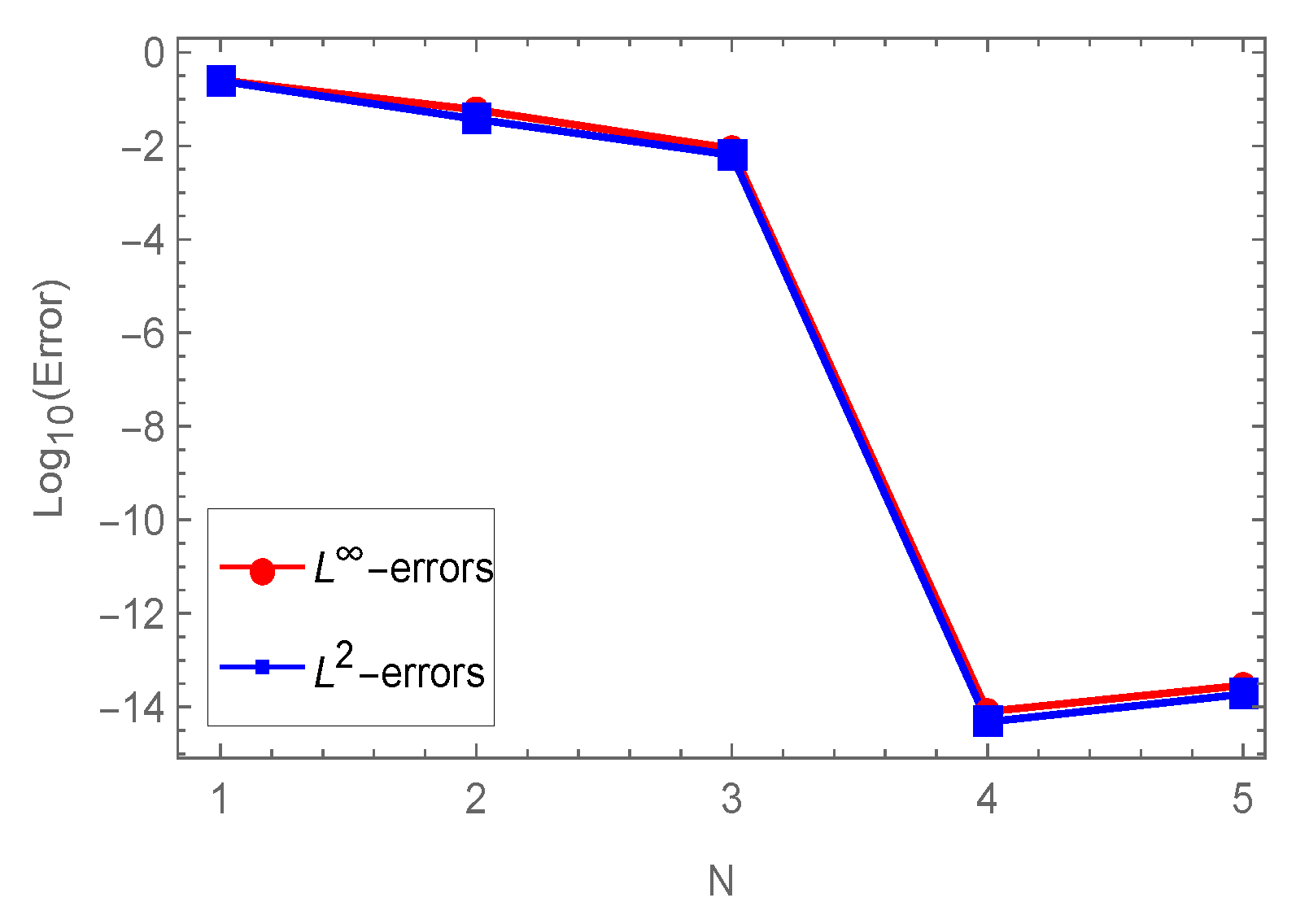
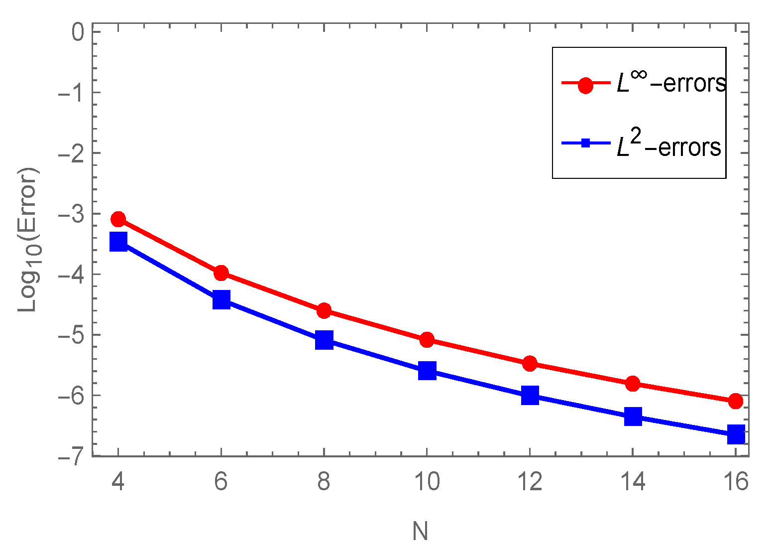
with those obtained by [41] and [42]. The results of this table ensure the superiority of our method when compared with the other two methods. Additionally, Figure 1 plots the maximum absolute error (MAE) of the solutions resulting from the application of our proposed algorithm for ${\upsilon }_1=0.5,b=0$ and $N=4$, while Figure 2 displays the $Lo{g}_{10}(L^{\infty }-errors)$ and $Lo{g}_{10}(L^2-errors)$ of our proposed algorithm for the case corresponds to: ${\upsilon }_1=0.25$ and $b=2$ with various values of N.

Remark 4.

From the data in Table 2, we can infer that the standard Chebyshev polynomials of the first kind are not the best approximations among the various classes of shifted polynomials $S{T}_i^b\left(x\right)$. This demonstrates the significance of our generalization to the first kind of Chebyshev polynomials and their shifted ones, and it also demonstrates the impact of the parameter b that occurs in the shifted polynomials.

Example 2.

Consider the following FDE [43]:

$${\mathcal{D}}_x^{{\upsilon }_1}\mathcal{Z}\left(x\right)+\mathcal{Z}\left(x\right)=x^2+\frac{2}{\mathsf{\Gamma }(3-{\upsilon }_1)}{x}^{2-{\upsilon }_1},0<{\upsilon }_1<1,$$

$$\mathcal{Z}\left(0\right)=0,$$

in which $\mathcal{Z}\left(x\right)=x^2$ is the exact solution.

Several methods have been developed to treat numerically this problem. Bonab and Javidi [43] proposed some explicit methods based on the fractional backward differentiation method (FBDM) of order three for the numerical solution of the current problem. We applied our algorithm for obtaining the numerical solution to this problem. In

Table 3. $L^{\infty }$-errors of our algorithm at ${\upsilon }_1=0.5$ and $N=2$ with distinct b for Example 2.

b	${\mathit{L}}^{\mathbf{\infty }}$-Errors
0	$1.21431\times {10}^{-16}$
1	$1.11022\times {10}^{-16}$
2	$6.93889\times {10}^{-16}$
3	$3.60822\times {10}^{-16}$
4	$4.16334\times {10}^{-16}$
5	$6.66134\times {10}^{-16}$

, the $L^{\infty }$-errors resulting from that application of our algorithm are presented for the case corresponding to ${\upsilon }_1=0.5$ and $N=2$ with distinct b. Furthermore,

Table 4. Comparison of $L^{\infty }$-errors of our algorithm at ${\upsilon }_1=0.7,0.8$ and $b=1$ for $N=2$ with the FBDM [43] for Example 2.

		FBDM [43]			Our Method
${\mathbf{\upsilon }}_{\mathbf{1}}$	$\mathit{h}\mathbf{=}\mathbf{0.1}$	$\mathit{h}\mathbf{=}\mathbf{0.01}$	$\mathit{h}\mathbf{=}\mathbf{0.001}$		$\mathit{N}\mathbf{=}\mathbf{2}$
0.7	$2.50\times {10}^{-3}$	$9.62\times {10}^{-6}$	$4.74\times {10}^{-8}$		$7.63\times {10}^{-16}$
0.8	$4.20\times {10}^{-3}$	$2.00\times {10}^{-5}$	$1.23\times {10}^{-7}$		$2.22\times {10}^{-16}$

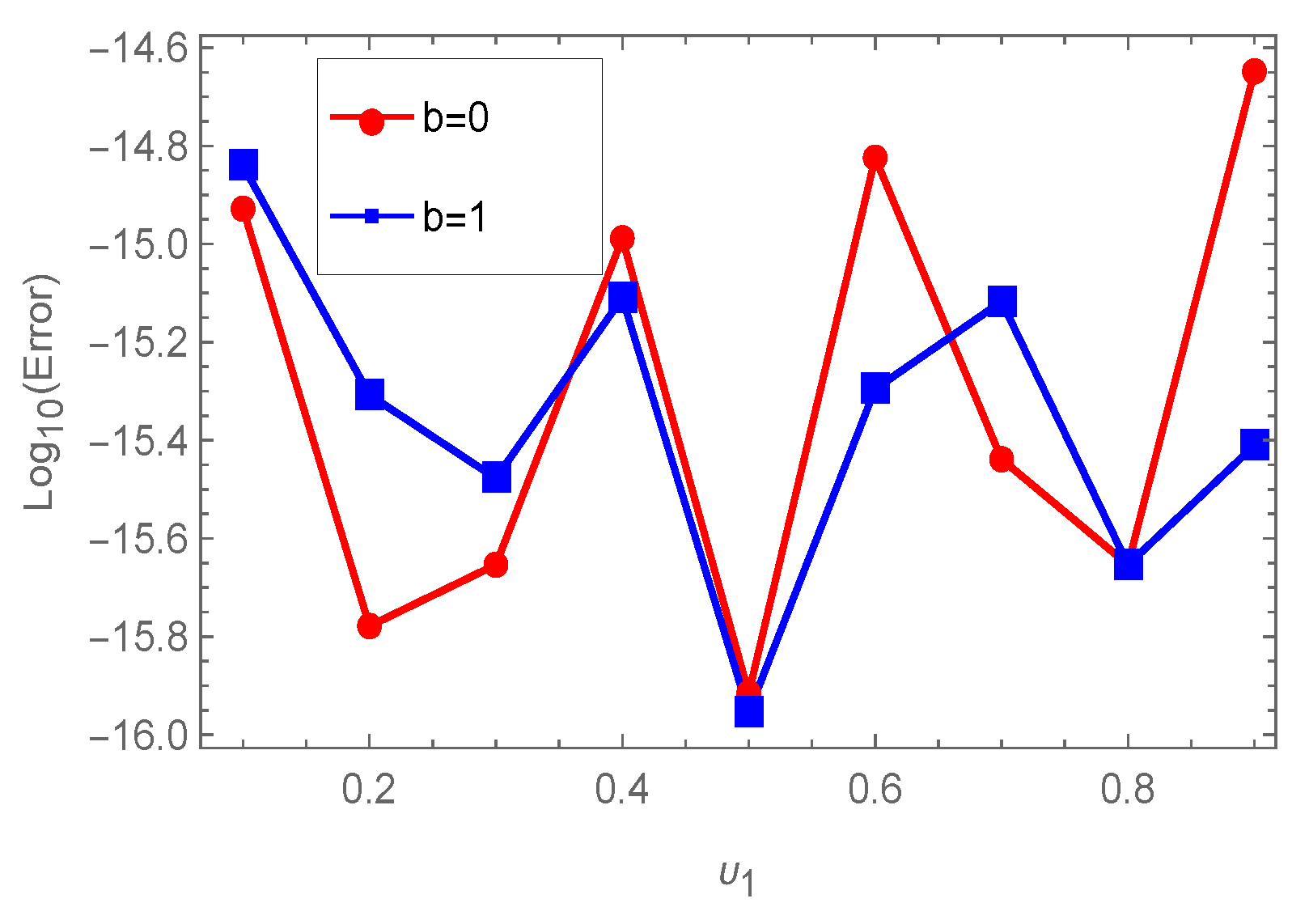
gives a comparison of $L^{\infty }$-errors resulting from our algorithm for ${\upsilon }_1=0.7,0.8$ and $b=1$ for $N=2$ with the FBDM that developed in [43] (h is the mesh size). Furthermore, to illustrate the influence of the parameter b, we compare in Figure 3 the resulting $Lo{g}_{10}(L^{\infty }-errors)$ of our algorithm for $b=0$ and $b=1$, $N=2$ with distinct ${\upsilon }_1$. Figure 4 and Figure 5 give the MAE of ${\mathcal{Z}}_N\left(x\right)$ of our algorithm at respectively: ${\upsilon }_1=0.7$, $b=1,N=2$ and ${\upsilon }_1=0.8$ and $b=1,N=2$.

Example 3.

Consider the following FDE [44]:

$${\mathcal{D}}_x^{{\upsilon }_1}\mathcal{Z}\left(x\right)+2\mathcal{Z}\left(x\right)=2cos\left(\pi x\right)+\frac{t^{-{\upsilon }_1}}{2\mathsf{\Gamma }(1-{\upsilon }_1)}\left({}_1{F}_1(1;1-{\upsilon }_1;i\pi x){.}_1{F}_1(1;1-{\upsilon }_1;-i\pi x)\right)-2,0<{\upsilon }_1<1,$$

$$\mathcal{Z}\left(0\right)=1,$$

exact solution $\mathcal{Z}\left(x\right)=cos\left(\pi x\right)$.

Table 5. Comparison of $L^{\infty }$- and $L^2$-errors of our algorithm at ${\upsilon }_1=0.5$ and $N=15$ with distinct b for Example 3.

b	${\mathit{L}}^{\mathbf{\infty }}$-Errors	${\mathit{L}}^{\mathbf{2}}$-Errors
0	$1.11022\times {10}^{-15}$	$7.37610\times {10}^{-17}$
1	$1.77636\times {10}^{-15}$	$7.07907\times {10}^{-17}$
2	$9.99201\times {10}^{-16}$	$7.08155\times {10}^{-17}$
3	$1.77636\times {10}^{-15}$	$7.13179\times {10}^{-17}$
4	$1.66533\times {10}^{-15}$	$7.18620\times {10}^{-17}$
5	$1.44329\times {10}^{-15}$	$7.23560\times {10}^{-17}$

displays a comparison of $L^{\infty }$- and $L^2$-errors of our algorithm at ${\upsilon }_1=0.5$ and $N=15$ with distinct b, while

Table 6. Comparison of $L^{\infty }$-errors of our algorithm for ${\upsilon }_1=0.5$ and $b=0$ with the Tau method in [44] by the approximate solution of degree M for Example 3.

$\mathcal{O}({\mathit{L}}^{\mathbf{\infty }}-\mathit{errors})$	LTM [44]			CTM [44]			Our Method
	M of LGL Points	M of $\mathbf{[}\mathbf{0}\mathbf{,}\mathbf{1}\mathbf{]}$		M of CGL Points	M of $\mathbf{[}\mathbf{0}\mathbf{,}\mathbf{1}\mathbf{]}$		M
${10}^{-07}$	−	−		09	−		07
${10}^{-09}$	11	11		11	11		09
${10}^{-11}$	13	13		13	13		11
${10}^{-14}$	−	−		−	−		13
${10}^{-15}$	−	−		−	−		15

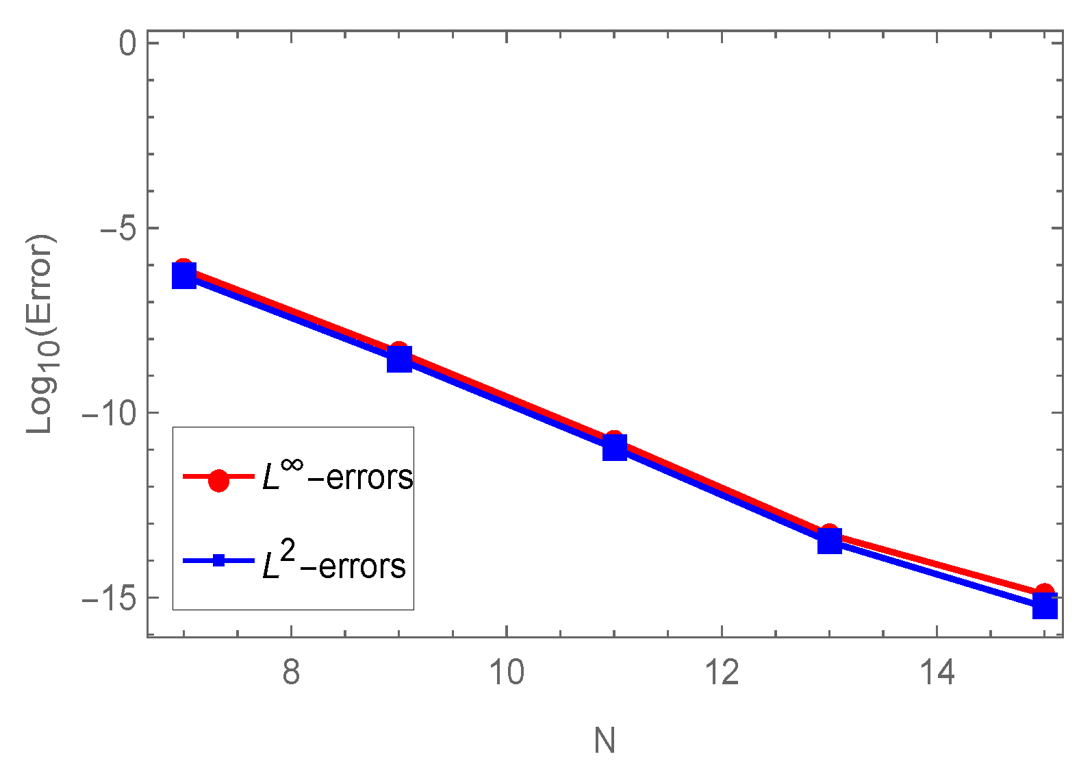
compares $L^{\infty }$-errors of our algorithm for ${\upsilon }_1=0.5$ and $b=0$ with the Tau method applied in [44], which were based using Chebyshev and Legendre namely, “Legendre–Gauss–Lobatto (LGL) points” and “Chebyshev–Gauss–Lobatto (CGL) points” by the approximate solution of degree M. Figure 6 plots the $Lo{g}_{10}(L^{\infty }-errors)$ and $Lo{g}_{10}(L^2-errors)$ resulted from the application of our algorithm at ${\upsilon }_1=0.5$ and $b=0$ with distinct N. 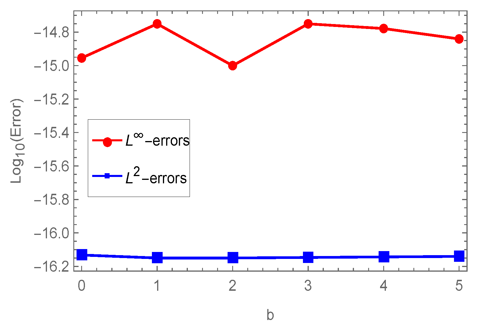Figure 7 displays the $Lo{g}_{10}(L^{\infty }-errors)$ and $Lo{g}_{10}(L^2-errors)$ of our algorithm at ${\upsilon }_1=0.5$ and $N=15$ with distinct b. Figure 8 shows the MAE of ${\mathcal{Z}}_N\left(x\right)$ of our proposed algorithm for ${\upsilon }_1=0.5$ and $N=15$ with $b=0$ (figure at left) and $b=2$ (figure at right).

Example 4.

Consider the following linear initial value problem [41]:

$${\mathcal{Z}}^{\prime }\left(x\right)+{\mathcal{D}}_x^{{\upsilon }_1}\mathcal{Z}\left(x\right)+\mathcal{Z}\left(x\right)=\frac{5}{2}{x}^{\frac{3}{2}}+x^{\frac{5}{2}}+\frac{15}{8}\frac{\sqrt{\pi }}{\mathsf{\Gamma }\left(\frac{13}{4}\right)}{x}^{\frac{9}{4}},$$

with the initial condition

$$\mathcal{Z}\left(0\right)=0.$$

The exact solution of this problem is $\mathcal{Z}\left(x\right)=x^2\sqrt{x}.$

Table 7. Comparison of $L^{\infty }$- and $L^2$-errors of our algorithm at ${\upsilon }_1=0.5$ and $N=20$ with distinct b for Example 4.

b	${\mathit{L}}^{\mathbf{\infty }}$-Errors	${\mathit{L}}^{\mathbf{2}}$-Errors
0	$2.64986\times {10}^{-7}$	$7.13878\times {10}^{-8}$
1	$1.64009\times {10}^{-7}$	$4.58693\times {10}^{-8}$
2	$1.32802\times {10}^{-7}$	$4.08146\times {10}^{-8}$
3	$1.21717\times {10}^{-7}$	$3.74664\times {10}^{-8}$
4	$1.40818\times {10}^{-7}$	$3.74237\times {10}^{-8}$
5	$1.35236\times {10}^{-7}$	$3.74547\times {10}^{-8}$

compares the $L^{\infty }$- and $L^2$-errors of our algorithm at ${\upsilon }_1=0.5$ and $N=20$ with distinct b, while

Table 8. Comparison of $L^{\infty }$- and $L^2$-errors of our algorithm for ${\upsilon }_1=0.5$ and $b=0$ with the CCSM in [41] by the approximate solution of degree M for Example 4.

$\mathcal{O}\left(\mathit{errors}\right)$	CCSM [41]		Our Method		CCSM [41]		Our Method
	M of ${\mathit{L}}^{\mathbf{\infty }}$-Errors		M of ${\mathit{L}}^{\mathbf{\infty }}$-Errors		M of ${\mathit{L}}^{\mathbf{2}}$-Errors		M of ${\mathit{L}}^{\mathbf{2}}$-Errors
${10}^{-3}$	5		4		−		4
${10}^{-4}$	−		5		5		5
${10}^{-5}$	9		8		9		6
${10}^{-6}$	17		11		−		9
${10}^{-7}$	21		17		17		13
${10}^{-8}$	−		−		−		20

gives a comparison of $L^{\infty }$- and $L^2$-errors of our algorithm for ${\upsilon }_1=0.5$ and $b=0$ with the CCSM that proposed in [41] by the approximate solution of degree M. Figure 8 displays the MAE of ${\mathcal{Z}}_N\left(x\right)$ of our algorithm for ${\upsilon }_1=0.5$ and $N=15$ with $b=0$ (figure at left) and $b=2$ (figure at right). Figure 9 displays the $Lo{g}_{10}(L^{\infty }-errors)$ and $Lo{g}_{10}(L^2-errors)$ of our algorithm at ${\upsilon }_1=0.5$ and $b=0$ with distinct N. Figure 10 describes the $Lo{g}_{10}(L^{\infty }-errors)$ and $Lo{g}_{10}(L^2-errors)$ of our algorithm at ${\upsilon }_1=0.5$ and $N=20$ with distinct b. Finally, Figure 11 displays the MAE of ${\mathcal{Z}}_N\left(x\right)$ of our algorithm for ${\upsilon }_1=0.5$ and $N=20$ with $b=0$ (figure at left) and $b=3$ (figure at right).

6. Conclusions

The spectral Galerkin method was utilized to treat multi-term FDEs governed by their initial conditions. Shifted generalized Chebyshev polynomials of the first kind were a newly introduced type that was used as basis functions. The Galerkin method was used to convert the FDE governed by its initial conditions into a linear matrix system with explicitly stated elements. Using a suitable numerical solver, this system of equations could be solved. Additionally, a few test examples were displayed to ensure the applicability and accuracy. As an important note, the case that corresponds to the standard shifted first-kind Chebyshev polynomials is not always better than the other special polynomials of our introduced generalized polynomials. To the best of our knowledge, this is the first time that differential equations were solved using these generalized polynomials. In upcoming work, we intend to use these orthogonal polynomials to solve a number of differential equations.