Abstract
The Poisson-stopped sum of the Hurwitz–Lerch zeta distribution is proposed as a model for interarrival times and rainfall depths. Theoretical properties and characterizations are investigated in comparison with other two models implemented to perform the same task: the Hurwitz–Lerch zeta distribution and the one inflated Hurwitz–Lerch zeta distribution. Within this framework, the capability of these three distributions to fit the main statistical features of rainfall time series was tested on a dataset never previously considered in the literature and chosen in order to represent very different climates from the rainfall characteristics point of view. The results address the Hurwitz–Lerch zeta distribution as a natural framework in rainfall modelling using the additional random convolution induced by the Poisson-stopped model as a further refinement. Indeed the Poisson contribution allows more flexibility and depiction in reproducing statistical features, even in the presence of very different climates.
1. Introduction
Analysis of rainfall data, and the subsequent modelling of the many variables concerning rainfall, is fundamental to many areas such as agricultural, ecological and engineering disciplines. From assessing hydrological risk to both crop and hydropower plannings, rainfall modelling is of the utmost importance. Moreover, being able to provide reliable rainfall modelling is essential in the well known issue of climate change. Due to the complexity of hydrological systems, their analysis and modelling rely heavily on historical records. Rainfall historical records are of various time scales, from hourly data to annual data. However, daily rainfall series are arguably the most used information in environmental, climate, hydrological, and water resources studies [1]. Rainfall manifests one peculiar characteristic which is common to many other geophysical processes: intermittence [2]. Intermittence is found in variables which are related to the internal and external structure of rainfall. The most commonly seen for the external structure are the Wet Spells () and Dry Spells (), meaning the sequences of rainy days and non-rainy days, respectively. A way of studying the alternance of and is through the Interarrival Times (), that is the time elapsed between two consecutive days of rain. If we suppose that observations are independent and identically distributed (i.i.d.), one natural way to model them is through the well known renewal processes [3]. Many examples can be found in the literature. The simplest renewal process, the Bernoulli process, has been used in [4] for example. In this case, the ’s are geometrically distributed. Its continuous counterpart, the Poisson process, has been used for its simpler mathematical tractability, but requires dealing with the random variable (r.v.) as continuous, despite its discrete nature. The need to suppose a non-constant probability of rain requires slightly more sophisticated models.
The challenge of this paper is to propose a suitable discrete distribution to fit at the daily scale. It is on this time scale that the intermittent character of precipitation can be appreciated and at the same time most practical applications are possible. The proposed distribution must be able to model both the numerous occurrences of the value equal to one, which represent the sequence of rainy days, and some large values scattered over time and responsible for drought phenomena. Our starting point is the three parameter family Hurwitz–Lerch Zeta distribution (HLZD), successfully proposed in [5]. Such a distribution represents a step forward with respect to other commonly used modelling distributions, such as the logarithmic one. In Section 3, we summarize the main properties of the HLZD and state new results on its log-concavity and convolution. As a step forward, in this paper we propose to model the r.v. using the Poisson-stopped HLZD (PSHLZD). This discrete distribution presents excess zeroes (paralleling the excess of ) and a long tail [6]. The PSHLZD has been used in [6] for comparisons with the negative binomial distribution, a popular model for fitting over-dispersed data. Indeed the PSHLZD can be seen both as a Poisson-stopped sum of HLZD’s as well as a generalization of a negative binomial distribution. The Poisson contribution allows us to model the superposition of i.i.d. HLZD’s in the observed time series as rare event. In Section 4, we summarize its main properties using the combinatorics of exponential Bell polynomials. It is noteworthy to mention that Bell polynomials are used within fractional calculus, see for example [7,8] and within fractal models [9]. Moreover, new results are added on the the PSHLZD, as for example on log-concavity.
A second goal of this paper is to show that the PSHLZD is also a suitable model for a different feature strictly related to the internal structure of rainfall: the depth (or the intensity) of the rainy days [10]. In the literature, refs. [11,12] rainfall depths are more often treated as continuous despite that sometimes these models fail to account for the time discreteness of the sample process [13]. Daily rainfall depth measurements are almost always performed by automatically counting how many times a small bucket corresponding to mm is filled. This led use to treat them as discrete, because of the abundance of ties in the data. Finally, in Section 5 we have also considered a third modelling distribution: the One Inflated HLZD (OIHLZD). Such a distribution mixes two generating processes: the first generates one’s and the latter is governed by a HLZD. This stochastic structure takes into account the dominance of one’s in the rainfall depth or interarrival time series.
In Section 6, we discuss the results for fitting all these models to rainfall data, proving that the PSHLZD provides a very general framework for rainfall modelling. Indeed the PSHLZD replicates the fitting features of the OIHLZD and outperforms the fitted HLZD in some cases. The PSHLZD has a limited number of parameters and at the same time can adapt very well to data collected in very different climates, from England to Sicily. Let us underline that the analyzed dataset has never been considered in the literature and consists of measures sampled along 70 years at 5 different stations. These stations were chosen in order to represent different climates from the rainfall characteristics point of view. In fact, the interarrival data examined are very different from each other, with a regular pattern of many rainy days in England, and a winter rainy season alternating with long periods in summer without rain, typical of the Sicily Mediterranean climate. The same is for the rainfall depth, namely many small depths in England, and few big storms in Sicily. This made it possible to confirm the great utility of the proposed statistical models within rainfall modelling. Some concluding remarks and future developments are addressed at the end of the paper.
2. Bell Polynomials in a Nutshell
The partial exponential Bell polynomials are usually written as [14]
where the summation is over all the solutions in non-negative integers of and A lighter expression is obtained using partitions of the integer n with length Recall that a partition of an integer n is a sequence of weakly decreasing positive integers, named parts of such that A different notation is where named multiplicities of are the number of parts of equal to respectively. The length of the partition is and the vector of multiplicities is We write to denote that is a partition of Thus the partial exponential Bell polynomials (1) can be rewritten as [15]
where the sum is over all the partitions with length and
Using integer partitions, the explicit expression of the partial exponential polynomials can be recovered in R using the kStatistics package [16]. A useful property used in the following is
with constants. Equation (4) follows from (2) since from (3) we have
taking into account that and
The n-th complete exponential Bell polynomials in the indeterminates is defined as [14]
with the partial exponential Bell polynomials (1). Note that n is the positive integer corresponding to the maximum degree of the monomials in (5). This polynomial sequence satisfies the following recurrence [14]
with the initial value The generating function of is the formal power series composition [14]
where is the ring of formal power series in t and is the generating function of , that is
A different expression of the n-th complete exponential Bell polynomial involves integer partitions [15] as follows
where the sum is over all the partitions and are given in (3). In particular we have
with a constant. Now, suppose to replace in (9) with a numerical sequence Thanks to this device, the complete exponential Bell polynomials results as a special case of a wider class of polynomial families, the generalized partition polynomials [16]
where the sum is again over all the partitions A different expression of (10) involves the partial exponential Bell polynomials in (1)
An example of a well known polynomial family, arising from (11) is the logarithmic one [14]
3. The Hurwitz-Lerch Zeta Distribution
Definition 1.
A discrete random variable if
for with , where
is the Lerch Transcendent function.
The probability generating function (pgf) of is
with
3.1. Moments and Cumulants
HLZD moments have a closed form expression involving the Lerch Transcendent function. Differently from [17], we find this closed form expression using (13).
Proposition 1.
If , then
Proof.
As a corollary, the mean and the variance are respectively:
More generally, the k-th central moment can be recovered as
and the factorial moments as
with Stirling numbers of the first kind [14]. HLZD cumulants are such that [14]
where are the moments of given in (16), and is the n-th logarithmic polynomial (12). Let us recall that, if the moment generating function (mgf) of Y is well defined in a suitable neighborhood of then the coefficients in the expansion
are the cumulants of The first cumulant is the mean the second cumulant is the variance the skewness and the kurtosis of Y can be recovered using the third and the fourth cumulant of Y respectively.
3.2. Mode
The HLZ distribution is a particular case of a wider class of distributions called the Modified Power Series Distributions (MPSD) [18].
Definition 2.
A discrete random variable if
where , and are positive, bounded, and differentiable functions of y and θ respectively with
Using this wider class of distributions, we will prove that is unimodal for all To this aim, let us recall that a discrete distribution with support is said to be strongly unimodal if and only if the sequence with is a logarithmically concave sequence [19], that is if and only if
Proposition 2.
Suppose
- If the sequence is monotonically decreasing and the mode is .
- If Y is strongly unimodal.
3.3. Convolution
The family of HLZ distributions is not closed under convolution. Nevertheless, as a subclass of MPS distributions, the HLZD convolution still returns a MPSD. Indeed we will prove that the family of MPS distributions is closed under convolution.
Theorem 1.
If are independent r.v.’s identically distributed to then with and
and given in (3).
Proof.
Observe that if are r.v.’s i.i.d. to then with and
with Indeed in (18), set if and consider the sequence such that if By using Lemma 1 in [21], we have
where are the partial exponential Bell polynomials (1). From (23) with replaced by for and using (4) we have
Thus with and given in (22). From (24) note that if By replacing and for in (24) we have
The result follows after some manipulations, rewriting the partial Bell exponential polynomials as in (2). □
3.4. Maximum Likelihood Estimation
Consider a vector of independent observations of . The maximum likelihood estimation (MLE) of is
with the log-likelihood function and
The MLE of the HLZD parameters has been studied by Gupta in [20]. He showed that the three likelihood equations arising from maximizing the log-likelihood correspond to the equations of the method of moments. In particular we have
Unfortunately, closed form solutions of the above equations are not available and also the moments and must be numerically approximated. As noted in [20], the likelihood equations may be solved by standard numerical methods to obtain the MLE. However, it is well known that this does not guarantee that global maxima of the likelihood have been achieved. In order to avoid this problem, a global optimization method can be employed to solve (25). The global optimization method takes advantage of the bounds of the parameters. More specifically, the MLE of the parameters can be obtained through a global optimization algorithm known as Simulated Annealing [22]. Simulated annealing is a stochastic global optimisation technique applicable to a wide range of discrete and continuous variable problems. It makes use of Markov Chain Monte Carlo samplers, to provide a means to escape local optima by allowing moves which worsen the objective function, with the aim of finding a global optimum. Technical details can be found in [22], a variant of which is the algorithm implemented in the Optim function in the base Stats R-package.
4. The Poisson-Stopped Hurwitz-Lerch Zeta Distribution
Definition 3.
A discrete random variable if its pgf is
where Φ is the Lerch Transcendent function (15).
According to Definition 3, takes non-negative integer values and belongs to the class of generalized r.v.’s [23]. Indeed given two independent r.v.’s Z and with pgf and respectively, the generalized r.v. X has pgf
The composition (26) matches (27) when and Z is a Poisson r.v. (PS) of parameter independent of since
In the following we analyse in detail the properties of the PSHLZD using the complete exponential Bell polynomials. Some of the properties given in [6] will also be briefly recalled.
Proposition 3.
If then
where is the complete exponential Bell polynomial (5) of degree
Corollary 1.
As a corollary of Proposition 3 and recursion (6), the sequence in (28) satisfies the following equations.
Corollary 2.
If then
Proof.
The result follows using (6) since we have
□
The PSHLZD is unimodal if and ([6], Property 1).
4.1. Log-Concavity
Under suitable conditions, the PSHLZD is log-concave.
Proposition 4.
If and then X has a log-concave cumulative distribution function (cdf), that is
Proof.
According to ([24], Theorem 1), a random sum of i.i.d. r.v.’s has a log-concave cdf if Z is strongly unimodal and the distribution of has a decreasing pdf. Thus, the result follows as with which has a log-concave pdf (strongly unimodal), and with a decreasing pdf when (see Proposition 2). □
Proposition 4 gives a sufficient condition to get cdf log-concavity. A different way is to consider the sequence Indeed, if X has a log-concave pdf (19), then its cdf is also log-concave [24]. In the more general setting of generalized r.v.’s, X has a log-concave pdf if and only if the sequence
is log-concave with and Equation (30) follows from Equation (2.3) in [23] using the general partition polynomials (8). When a necessary and sufficient condition to recover strong unimodality is related to the magnitude of and as the following theorem shows.
Theorem 2.
If X is a generalized r.v. with Y strongly unimodal and then X is strongly unimodal if and only if .
Note that a similar result is proved in ([25], Theorem 4). We provide a different proof using the following lemma.
Lemma 1.
If is a log-concave sequence, then the sequence is log-concave if and only if with given in (5).
Proof.
If with is a log-concave sequence of non-negative real numbers and the sequence is defined by
then the sequence is log-concave [26]. Equation (31) parallels (7). Therefore, the sequence results as log-concave if the sequence is log-concave. Note that for we have
which easily reduces to always satisfied when is log-concave. Now let . We have is log-concave if and only if and the result follows. □
Proof
(Proof of Theorem 2). Following the same arguments of Proposition 3, for a generalized r.v. with (30) reduces to
with for The sequence is log-concave if and only if the sequence is log-concave. The result follows using Lemma 1. □
Corollary 3.
If is strongly unimodal if and only if
4.2. Moments and Cumulants
PSHLZD moments and cumulants have closed form expressions in terms of moments of
Proposition 5.
If then
Proof.
Remark 1.
Taking into account (33), if then with and that is X is a compound Poisson r.v. Therefore the PSHLZD is an infinitely divisible distribution [27].
Moments (32) can be explicited written using (9). A straightforward corollary of recursion (6) is the following.
Corollary 4.
If denotes the k-th central moment of then
Proposition 6.
If then
where are the first k factorial moments of given in (17).
Proof.
Proposition 7.
If is the n-th cumulant of then for where is the n-th moment of given in (16).
Proof.
The result follows since
□
4.3. Maximum Likelihood Estimation
Suppose to have independent observations of The MLE of is
with the log-likelihood function and
The MLE of the PSHLZD parameters in this case must be directly tackled with the global optimization method described in Section 3.4, since is not analytically tractable referring to (29).
5. The One Inflated Hurwitz-Lerch Zeta Distribution
Definition 4.
A discrete random variable if
with and
This definition parallels the definition of the Zero Inflated Modified Power Series Distribution given by Gupta [28]. If denotes the pgf of then
and the HLZD is retrieved by setting
5.1. Moments and Cumulants
Similarly, if is the factorial mgf of since with the factorial mgf of then
with the k-th factorial moment of given in (17).
5.2. Maximum Likelihood Estimation
To estimate the OIHLZD parameters using the MLE, let us first rewrite (36) using (18), that is
where and Rewrite (39) as
where W has a One Truncated Hurwitz-Lerch Zeta Distribution (OTHLZD) [29], that is
Suppose is a vector of independent observations of and is the log-likelihood function with
If is the number of times the integer j appears in the vector for then the log-likelihood can be written as
Now set
and
From (41) and (42), the parameters can be estimated separately, that is the estimation can be recovered from and the estimations from . The latter ones give the MLE of the parameters of in (40) using the vector restricted to the observations which are greater than As a consequence, the estimation of p can be recovered from as
6. Data-Fitting
6.1. Rainfall Depths and Interarrival Times
With rainfall depth we indicate to what depth liquid precipitation would cover a horizontal surface in an observation period if nothing could drain, evaporate or percolate from this surface. Let a time series of rainfall data be defined as , where h (mm) is the rainfall depth recorded at a fixed uniform unit of time (e.g., a day). A day k is considered rainy if the rainfall depth , where is a fixed rainfall threshold. The sub-series of h of the rainy days can be defined as the event series , where is an integer multiple of the time-scale . The sequence built with the times elapsed between each element of E (except the first one) and the immediately preceding one is defined as the interarrival time series . In order to select an appropriate distribution for , some statistical characteristics usually observed in samples have to be considered: very high variance and skewness, relatively high frequency associated to the observation , monotonically decreasing frequencies with a slowly decaying tail and a drop in the passage from the frequency at to the one at . The HLZD in (13) has been fitted to rain in [5] for stations in Sicily and in [30] for stations in Piedmont, with good results. However, it has not yet been considered for rainfall depths. Recall that in the following we assume to model rainfall depths with a discrete r.v.
6.2. The Data
In this paper, the series analyzed were obtained from the recorded rainfall observations, using the rainfall threshold mm, which is the conventional threshold stated by the World Meteorological Organization in order to discriminate between rainy and non rainy days. This dataset has not been previously considered in the literature and consists of both and h measured over 70 years at the following five stations: Floresta, Trapani, Torino, Oxford, Ceva. They were chosen in order to represent different climates from the rainfall characteristics point of view. Floresta and Trapani represent the Mediterranean climate with a very wet and a very dry situation respectively. For both stations, the rainfall is concentrated in the colder part of the year, as typical of the Mediterranean climate. Torino and Ceva are more continental, but Ceva is more influenced by the Ligurian sea. Therefore, Torino has its maximum rain in Spring, while that of Ceva is in Autumn, because of the heating of the sea in the Summer. Finally, Oxford is a northern Europe station with rainfall homogeneously spread across the whole year. The recordings start in 1947 and end in 2017, for a total of 70 years. Moreover, the time series were further subdivided. Thus for each station we considered for a total of 33 samples. Note that we did not consider wet and dry seasons for Oxford station due to its climate.
More specifically let station_name∈ {Floresta, Trapani, Torino, Oxford, Ceva} and season_name∈ {wet, dry, spring, summer, autumn, winter}. Then the samples tagged with station_name year span the whole length of the series for the station_name station, while the samples tagged with station_name season_name are the union of all the season_name seasons in the whole time series for the station_name station, omitting all the other seasons from the dataset. The MLE was used to fit the HLZD (Section 3), the PSHLZD (Section 4) and the OIHLZD (Section 5) to the dataset (Note that the PSHLZD has support and the r.v. naturally has support so we had to consider the shifted r.v. .). In all cases, the MLE has been tackled with the method described in Section 3.4. The addressed global optimization procedure was further simplified by the previously mentioned statistical characteristics of the data allowing to work on a subset of the parameter space
- the whole time series, without subdividing the different seasons;
- all the wet seasons and all the dry seasons;
- the standard meteorological seasons,
6.3. Results
In the following we summarize the results of the distribution fitting for and h data. The fitting was satisfactory for both the PSHLZD and the HLZD. The assessment of the goodness-of-fit was obtained by following the methodology suggested by [31]. In the case of long tailed distributions, the goodness-of-fit through the classical test might be biased, because if there are several small classes, strong asymmetry might occur [31] and some problems of inaccuracy might appear if the classes are grouped [32]. The alternative procedure used to test the goodness-of-fit relies on Monte Carlo simulation to numerically reconstruct the null hypothesis of the test to compute the p-values [33].
To further inspect the differences between the distributions, we have measured the fitting errors whose magnitude is strictly related to the discrepancy between the empirical frequencies and the fitted ones. Since many empirical frequencies are zero (in the tail), the cdf has been considered. In particular we considered the mean absolute error (MAE) and the mean relative absolute error (MRAE). Let us recall that, if is an ordered sample, then and with the empirical cdf and the fitted cdf.
6.3.1. Interarrival Times
We have compared the fitted PSHLZD with the fitted HLZD and the fitted PSHLZD with the fitted OIHLZD. To summarize the results, we have selected 4 of the 33 available samples since they have been considered particularly meaningful with respect to the whole dataset. The selected samples were Floresta Summer, Trapani Wet, Trapani Dry and Torino Winter.
Figure 1 is an example of empirical frequencies: they usually range from a high peak located at to a multitude of rather smaller values in the slow decaying tails. Therefore, to perform comparisons, a log-log scale for all the plots has been adopted.
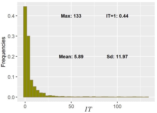
Figure 1.
Histogram of the empirical frequency for the Trapani station over the whole year. The range is up to The mode is with relative frequency The mean and the standard deviation are and respectively.
Figure 2 shows plots of the fitted PSHLZD (solid line) and HLZD (dotted line) compared with the empirical frequencies (dot line) for the 4 selected samples. The fitting in both cases is very good. In particular, in the cases of Floresta Summer, Torino Winter and Trapani Dry the PSHLZD succeeds in fitting the drop from to whereas the HLZD fails. This happens in the drier periods, where this drop is more prominent.
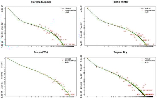
Figure 2.
Log-log plots of the fitted HLZD (green dotted line), the fitted PSHLZD (black solid line) and the empirical frequencies (red dot line) for the 4 selected samples Floresta Summer, Torino Winter, Trapani Wet and Trapani Dry.
Moreover, Figure 1 shows the dominance of the frequencies corresponding to and which are particularly meaningful in hydrology. Figure 3 shows the plots of MAE and MRAE obtained by comparing the fitted cdf’s of the PSHLZD (circle) and the HLZD (triangle) with the empirical cdf’s. Note that the MAE and the MRAE are in general lower for the PSHLZD. Due to the dominance of the frequency corresponding to we explored modelling with the OIHLZD for all the samples. In all cases, the fitted OIHLZD and the PSHLZD one have minimal differences and are almost indistinguishable (see Figure 4 for an example), confirming the great flexibility of the latter distribution.
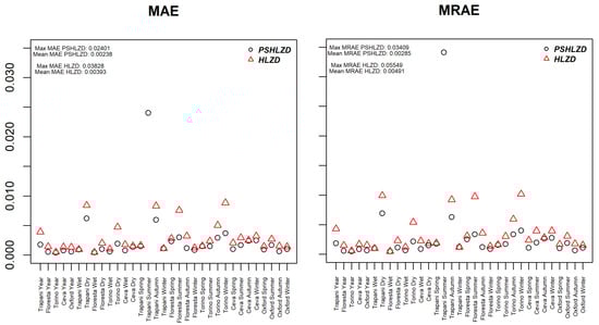
Figure 3.
Dot plots of MAE and MRAE taking as reference the cdf of the PSHLZD (black circle) and of the HLZD (red triangle) for all the samples. The maximum MAE as well as the mean MAE are given in the top left for both the fitting distributions.
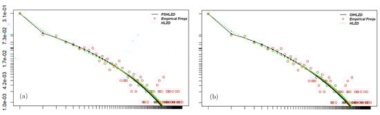
Figure 4.
(a), the fitted PSHLZD (black solid line) is plotted together with the fitted HLZD (green dotted line) and the empirical frequencies (red dot line) for the sample of Trapani Dry. (b) the fitted OIHLZD (black solid line) is plotted together with the fitted HLZD (green dotted line) and the empirical frequencies (red dot line) for the same sample.
To conclude the validation analysis, we compared sample means and sample variances with the same theoretical moments of the HLZD and the PSHLZD computed in Section 3 and Section 4 respectively. In Table 1, we show the results for the 4 selected samples. In all cases, the fitted distributions agree with the sample means. For the variances, the PSHLZD performs better in many cases. In Table 1, an exception is Trapani Wet because the data are highly dispersed.

Table 1.
The sample means and the sample variances for the 4 selected samples are given in the first column. The means and the variances of the fitted HLZD and of the fitted PSHLZD are given in the second and in the third column respectively.
6.3.2. Rainfall Depths
In this section, we summarize the fitting of the rainfall depth time series using both the PSHLZD and the HLZD. We omit the comparison with the OIHLZD since this distribution does not add more insights on the fitting nor what happens for the datasets.
Figure 5 shows again an empirical frequency histogram ranging from a high peak in to a multitude of rather smaller values in the slowly decaying tails. As in the previous section, we employed a log-log scale for all the plots. The selected samples were Ceva Winter, Torino Winter, Floresta Dry and Trapani Summer.
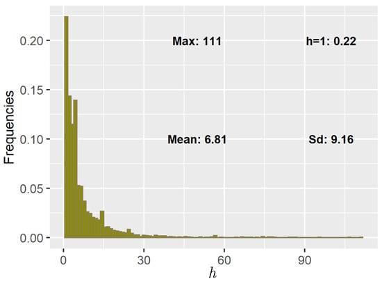
Figure 5.
Plot of the empirical h frequency histogram for the Trapani station over the whole year. 111 is the maximum registered depth. The mode is with relative frequency The mean and the standard deviation are and respectively.
In Figure 6 we have plotted the fitted PSHLZD and HLZD compared with the empirical frequencies. As with samples, the fitting is very good, even better that in the case. Moreover there is less difference between the performances of the PSHLZD and the HLZD.
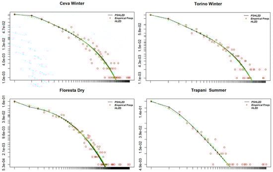
Figure 6.
Log-log plots of the fitted HLZD (green dotted line), the fitted PSHLZD (black solid line) and the h empirical frequencies (red dot line) for the 4 selected samples Ceva Winter, Torino Winter, Floresta Dry and Trapani Summer.
Figure 7 shows the plots of the MAE and the MRAE obtained by comparing the fitted cdf’s of the PSHLZD (circle) and the HLZD (triangle) with the empirical h cdf’s. Even though both errors are smaller for the PSHLZD, there is less difference between the two distributions and they are generally lower than for the case.
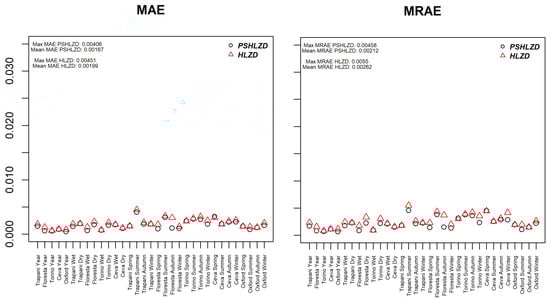
Figure 7.
Dot plots of MAE and MRAE taking as reference the cdf of the PSHLZD (black circle) and of the HLZD (red triangle) for all the h samples. The maximum MAE as well as the mean MAE are given in the top left for both the fitting distributions.
7. Conclusions
The first part of this paper focuses on a class of discrete distributions useful to describe very high one counts and long tails. We have reviewed the main properties using the combinatorics of exponential Bell polynomials. This device has permitted the derivation of closed form expressions for the pdf’s and their convolutions, as well as moments and cumulants. Moreover, new results on log-concavity have been presented. We have also considered the OIHLZD to compare its features with the HLZD and the PSHLZD. This deep analysis was aimed of investigating how to use these models to find a better fit for rainfall data. Indeed, the PSHLZD and the HLZD were fitted on Interarrival Times and rainfall depths h data coming from 5 different stations, which composed a dataset never previously analyzed in the literature. The h data were treated as observations of a discrete r.v., which is not the usual practice in the literature, but seems reasonable when taking into account how they are measured. The fitting was performed with the classical MLE method, but the likelihood was maximized using the Simulated Annealing procedure, which turns out to be fundamental since there are no closed forms of the likelihood equations. The fit was very good for both distributions, with the PSHLZD performing slightly better than the HLZD. This mostly happens for the data. Moreover, the PSHLZD was also able to replicate the fit of the OIHLZD further validating its flexibility.
From the modelling point of view, let us underline two final remarks. Firstly, the fit was excellent for both the and the h data, suggesting that the PSHLZD can be proposed as a general framework in rainfall modelling. Secondly, it is noteworthy to underline that these models capture the variability of rainfall stochastic phenomena, even though the 5 considered stations represent very different climates: a case study not yet considered in the literature that deals with previous applications of HLZD. Future works will consider modelling the dependence (inter-correlation) between and h. Given the remarkable performance of these distribution families in the univariate modelling, a first step would be to consider bivariate modified power series distributions [34] and the methods to estimate their parameters on a rainfall time series. This is in the agenda for our future developments.
Author Contributions
Conceptualization, C.A., G.B., S.F., E.D.N. and T.M.; methodology, E.D.N. and T.M.; software, T.M.; validation, E.D.N. and T.M.; formal analysis, E.D.N. and T.M.; data curation, C.A., G.B. and S.F.; writing—original draft preparation, E.D.N. and T.M.; writing—review and editing, C.A., G.B., S.F., E.D.N. and T.M.; funding acquisition, S.F. All authors have read and agreed to the published version of the manuscript.
Funding
This research was funded by MIUR—Dipartimento di Eccellenza- DIST department funds, and by the “PRIN MIUR 2017SL7ABC_005 WATZON Project”.
Data Availability Statement
Data are available upon request to the Società Italiana di Meteorologia.
Acknowledgments
The authors would like to thank the anonymous referees and the associate editor for carefully reading this manuscript and giving valuable comments to improve the previous version of this paper. The authors would like to thank Nicholas Howden of University of Bristol and Daniele Cat Berro and Luca Mercalli of Società Meteorologica Italiana to provide the English and North-Italy rainfall time series. The authors would like to thank the “Risk Responsible Resilience Interdepartmental Centre” (R3C).
Conflicts of Interest
The authors declare no conflict of interest.
References
- Serinaldi, F. A multisite daily rainfall generator driven by bivariate copula-based mixed distributions. J. Geophys. Res. Atmos. 2009, 114, D10103. [Google Scholar] [CrossRef]
- Davis, A.; Wiscombe, W.; Cahalan, R.; Marshak, A. Multifractal characterizations of nonstationary and intermittency in geophysical fields: Observed, retrieved, or simulated. J. Geophys. Res. 1994, 99, 8055–8072. [Google Scholar] [CrossRef]
- Lawrance, A.J. Stochastic Modelling of Daily Rainfall Sequences. J. R. Stat. Soc. Ser. C Appl. Stat. 1979, 28, 84. [Google Scholar] [CrossRef][Green Version]
- Chatfield, C. Wet and dry spells. Weather 1966, 21, 308–310. [Google Scholar] [CrossRef]
- Agnese, C.; Baiamonte, G.; Cammalleri, C. Modelling the occurrence of rainy days under a typical Mediterranean climate. Adv. Water Resour. 2014, 64, 62–76. [Google Scholar] [CrossRef]
- Liew, K.W.; Ong, S.H.; Toh, K.K. The Poisson-stopped Hurwitz–Lerch zeta distribution. Commun. Stat.—Theory Methods 2022, 51, 5638–5652. [Google Scholar] [CrossRef]
- Liu, M.; Zhang, L.; Fang, Y.; Dong, H. Exact solutions of fractional nonlinear equations by generalized bell polynomials and bilinear method. Therm. Sci. 2021, 25, 1373–1380. [Google Scholar] [CrossRef]
- Taghavian, H. The use of partition polynomial series in Laplace inversion of composite functions with applications in fractional calculus. Math. Methods Appl. Sci. 2019, 42, 2169–2189. [Google Scholar] [CrossRef]
- Fathizadeh, F.; Kafkoulis, Y.; Marcolli, M. Bell polynomials and Brownian bridge in spectral gravity models on multifractal Robertson–Walker cosmologies. In Annales Henri Poincaré; Springer: Berlin/Heidelberg, Germany, 2020; Volume 21, pp. 1329–1382. [Google Scholar]
- Bernardara, P.; De Michele, C.; Rosso, R. A simple model of rain in time: An alternating renewal process of wet and dry states with a fractional (non-Gaussian) rain intensity. Atmos. Res. 2007, 84, 291–301. [Google Scholar] [CrossRef]
- Yang, L.; Franzke, C.L.E.; Fu, Z. Power-law behaviour of hourly precipitation intensity and dry spell duration over the United States. Int. J. Climatol. 2020, 40, 2429–2444. [Google Scholar] [CrossRef]
- Porporato, A.; Vico, G.; Fay, P.A. Superstatistics of hydro-climatic fluctuations and interannual ecosystem productivity. Geophys. Res. Lett. 2006, 33, L15402. [Google Scholar] [CrossRef]
- Foufoula-Georgiou, E.; Lettenmaier, D.P. Continuous-time versus discrete-time point process models for rainfall occurrence series. Water Resour. Res. 1986, 22, 531–542. [Google Scholar] [CrossRef]
- Charalambides, C.A. Enumerative Combinatorics; CRC Press Series on Discrete Mathematics and its Applications; Chapman & Hall/CRC: Boca Raton, FL, USA, 2002; Volume 16, p. 609. [Google Scholar]
- Di Nardo, E.; Guarino, G.; Senato, D. A unifying framework for k-statistics, polykays and their multivariate generalizations. Bernoulli 2008, 14, 440–468. [Google Scholar] [CrossRef]
- Di Nardo, E.; Guarino, G. kStatistics: Unbiased Estimates of Joint Cumulant Products from the Multivariate Faà Di Bruno’s Formula. arXiv 2022, arXiv:2206.15348. [Google Scholar]
- Aksenov, S.V.; Savageau, M.A. Some properties of the Lerch family of discrete distributions. arXiv 2005, arXiv:math/0504485. [Google Scholar]
- Gupta, R.C. Modified power series distribution and some of its applications. Sankhyā Ser. B 1974, 36, 288–298. [Google Scholar]
- Keilson, J.; Gerber, H. Some Results for Discrete Unimodality. J. Am. Stat. Assoc. 1971, 66, 386–389. [Google Scholar] [CrossRef]
- Gupta, P.L.; Gupta, R.C.; Ong, S.H.; Srivastava, H. A class of Hurwitz–Lerch Zeta distributions and their applications in reliability. Appl. Math. Comput. 2008, 196, 521–531. [Google Scholar] [CrossRef]
- Eger, S. Identities for partial Bell polynomials derived from identities for weighted integer compositions. Aequationes Math. 2016, 90, 299–306. [Google Scholar] [CrossRef]
- Bélisle, C.J.P. Convergence theorems for a class of simulated annealing algorithms on Rd. J. Appl. Probab. 1992, 29, 885–895. [Google Scholar] [CrossRef]
- Charalambides, C.A. On the generalized discrete distributions and the Bell polynomials. Sankhyā Ser. B 1977, 39, 36–44. [Google Scholar]
- Badía, F.G.; Sangüesa, C.; Federgruen, A. Log-concavity of compound distributions with applications in operational and actuarial models. Probab. Eng. Inf. Sci. 2021, 35, 210–235. [Google Scholar] [CrossRef]
- Yu, Y. On the entropy of compound distributions on nonnegative integers. IEEE Trans. Inform. Theory 2009, 55, 3645–3650. [Google Scholar] [CrossRef]
- Bender, E.A.; Canfield, E.R. Log-concavity and related properties of the cycle index polynomials. J. Comb. Theory Ser. A 1996, 74, 57–70. [Google Scholar] [CrossRef]
- Sato, K.i. Lévy processes and infinitely divisible distributions. In Cambridge Studies in Advanced Mathematics; Translated from the 1990 Japanese original, Revised edition of the 1999 English translation; Cambridge University Press: Cambridge, UK, 2013; Volume 68, pp. 14, 521. [Google Scholar]
- Gupta, P.L.; Gupta, R.C.; Tripathi, R.C. Inflated modified power series distributions with applications. Commun. Stat.-Theory Methods 1995, 24, 2355–2374. [Google Scholar] [CrossRef]
- Conceição, K.S.; Louzada, F.; Andrade, M.G.; Helou, E.S. Zero-modified power series distribution and its Hurdle distribution version. J. Stat. Comput. Simul. 2017, 87, 1842–1862. [Google Scholar] [CrossRef]
- Baiamonte, G.; Mercalli, L.; Berro, D.C.; Agnese, C.; Ferraris, S. Modelling the frequency distribution of inter-arrival times from daily precipitation time-series in North-West Italy. Hydrol. Res. 2019, 50, 339–357. [Google Scholar] [CrossRef]
- Martínez-Rodríguez, A.M.; Sáez-Castillo, A.; Conde-Sánchez, A. Modelling using an extended Yule distribution. Comput. Stat. Data Anal. 2011, 55, 863–873. [Google Scholar] [CrossRef]
- Spierdijk, L.; Voorneveld, M. Superstars without talent? The Yule distribution controversy. Rev. Econ. Stat. 2009, 91, 648–652. [Google Scholar] [CrossRef]
- Hope, A.C. A simplified Monte Carlo significance test procedure. J. R. Stat. Soc. Ser. B Methodol. 1968, 30, 582–598. [Google Scholar] [CrossRef]
- Shoukri, M.M.; Consul, P.C. Bivariate Modified Power Series Distribution Some Properties, Estimation and Applications. Biom. J. 1982, 24, 787–799. [Google Scholar] [CrossRef]
Publisher’s Note: MDPI stays neutral with regard to jurisdictional claims in published maps and institutional affiliations. |
© 2022 by the authors. Licensee MDPI, Basel, Switzerland. This article is an open access article distributed under the terms and conditions of the Creative Commons Attribution (CC BY) license (https://creativecommons.org/licenses/by/4.0/).