Formal Verification of Fractional-Order PID Control Systems Using Higher-Order Logic

Abstract

Fractional-order PID control is a landmark in the development of fractional-order control theory. It can improve the control precision and accuracy of systems and achieve more robust control results. As a theorem-proving formal verification method, it can be applied to an arbitrary system represented by a mathematical model. It is the ideal verification method because it is not subject to limits on state numbers. This paper presents the higher-order logic (HOL) formal verification and modeling of fractional-order PID controller systems. Firstly, a fractional-order PID controller was designed. The accuracy of fractional-order PID control can be supported by simulation, comparing integral-order PID controls. Secondly, the superior property of fractional-order PID control is validated via higher-order logic theorem proofs. An important basic property, the relationship between fractional-order differential calculus and integral-order differential calculus, was analyzed via a higher-order logic theorem proof. Then, the relations between the fractional-order PID controller and integral-order PID controller were verified based on the fractional-order Grünwald–Letnikov definition for higher-order logic theorem proofs. Formalization models of the fractional-order PID controller and the fractional-order closed-loop control system were established. Finally, the stability of the fractional-order control systems was verified based on established formal models and theorems. The results show that the fractional-order PID controllers can be conducive to the control performance of control systems, and the higher-order logic formal verification method can ensure the reliability and security of fractional-order control systems.

1. Introduction

PID controllers are the most widely deployed in the procedure control industry [1,2,3,4,5,6,7,8]. PID controllers are now the first choice for the system’s bottom control. Fractional-order PID control is an expansion upon integral-order PID control, which allows the fractional-order to operate using integers outside of calculus [9,10]. Fractional-order PID controller was created by Professor I. Podlubny [11]. The fractional-order PID controller was a historical landmark in the fractional-order control theory and has laid a foundation for its further development. The fractional-order PID controller works on the basis of fractional-order differential calculus and a PID controller. Fractional-order differential calculus is a 300-year-old topic in mathematics. Fractional-order differential calculus is a straightforward way of extending conventional integral-order differential calculus, which permits the order to be a fraction [12,13,14,15]. The fractional-order controller provides more parameters and can improve precision. It is evident that conventional integral-order PID control is a unique implementation of fractional-order PID control [16]. Fractional-order PID control is used to increase the controlling accuracy of systems and get more robust control results.

In recent years, a lot of research has been conducted on fractional-order PID controllers. A novel optimization based on the adjustment approach to fractional-order PID controllers was introduced in [17]. The suggested approach was employed to devise a fractional-order PID controller to manage an undamped third-order system with a temporal lag, obtaining better ruggedness and other properties. An optimized fractional-order PID controller design policy was presented for a perpetual magnetic simultaneous machine service system on the basis of analysis calculations and difference evolvement algorithms in [18]. Velocity tracing simulations and trials indicated the remarkable benefits of the suggested fractional-order PID control with respect to the best fractional-order PI control and the conventional integral-order PID control. Fractional-order PID control has drawn a lot of interest from academic and industrial circles. The authors of [19] introduced a practical approach for adjusting fractional-order PID control. This adjustment approach was demonstrated on a high-technology precise-position system. Another fractional-order PID controller was devised for tuning the touch power of a dielectric friction detector for the quasi-active control of base isolation construction for far and near-site seismic stimulation [20]. The multiple goal booster searching operator was used to adjust the controller settings. According to the simulated data, the fractional-order PID controller outperforms others when it comes to simultaneously reducing the maximal basal displacements and the displacements of all kinds of seismic events. The authors of [21] proposed a multiple agency-based symbiosis search, which incorporates a multiple-agent subsystem into the symbiosis-seeking operator program for adjusting fractional-order PID control. The results validated the precision, robustness, and better properties of the presented approach over others. With respect to the worldwide energy management of pressurized, heavier waterpower reaction reactors in the regressive conditioning scenario, a robust fractional-order PID controller design method was presented in [22]. The simulated outcomes of the presented fractional-order PID control showed that the positive backstepping controls of the inserted bar have no overshoot and are reliable in terms of properties, as well as being secure against large changes in gain in the plant.

By tradition, emulation is the most employed technology for analyzing a fractional-order system. Due to the inaccurate nature of simulation, the analysis can never be precise. For some systems that require high-safety performance, especially those used in interactive worker robots, inaccurate results pose a serious threat and may even endanger lives, such as medical robots. There is no analytical solution when using the simulation method, and it is not a logical validation. The simulation method is not complete. To ensure higher safety performance, it is urgent for a more complete validation method. The higher-order logic (HOL) theorem-proof approach can verify the precision and superiority of an arbitrary fractional-order system, which is also a formal analysis method.

Formal analysis methods, as highly reliable techniques, have been successful in achieving precise analyses for both hardware and software [23]. Theorem proving is one such formal technique [24]. It formalizes mathematical concepts through precise semantics [25]. Many mathematical theories, including fractional-order calculus theory, can be safely expanded upon. Because of the high representational quality of higher-order logic theorem proving and the intrinsic rationality of theory proofs, this technique may be used to accurately analyze various fractional-order system models. Moreover, theorem proving can prevent the status spatial explosive issue [26]. NASA adopted the theorem prover PVS to formulate the control software specifications for space shuttles and their verification [27]. Four design errors were found, one of which was difficult to find by simulation and testing. The safety of autonomous robots was verified by the German Research Center for Artificial Intelligence based on a formalized theory called proving Isabelle [28]. Researchers there reported one successful endeavor concerning the designing, implementation, and certification of crash prevention security features for autonomous vehicles and stationary obstacles. In recent years, theory proofs have been employed satisfactorily for the precise analysis of some fractional-order system components. Study [29] presented the verification of a Gamma function and the fractional-order Riemann–Liouville definition. For illustration purposes, they provided the formalized analyses on a fractional-order electric element resisto-ductance, a fractional-order differentiator, and a fractional-order integrator loop.

In this article, fractional-order PID systems are shown to be verified through a formal, higher-order logic theory-proof approach. Formal verification is more accurate than simulation. According to the design method in [30], a fractional-order PID control was designed to control a robot. Then, the fractional-order PID controller was formalized using higher-order logic theory proofs. The relationship between fractional-order calculus and integral-order calculus has a critical impact on the verification of fractional-order PID controllers. This relationship was verified, firstly. The analyses of fractional-order PID controllers were predicated upon fractional-order Laplace transform. The formalized pattern of fractional-order Laplace transform was developed in HOL. Then the fractional-order PID controller was formalized. After fractional-order closed-loop control was formalized, the transformation from the frequent field to the temporal field was formally verified. Verification of this property became the foundation for the verification of many other performances of fractional-order closed-loop systems. On the basis of these results, we verified the fractional-order PID control of the robot which we designed. The result of the formal verification shows the correctness of the fractional-order controller and the validity of the formal theorem.

The major innovations of the article are presented below.

• The relationship between fractional-order calculus and integral-order calculus was verified in HOL. It serves as a theoretical foundation for the verification of fractional-order control;
• The formal model of fractional-order PID control was created, and the relationship between fractional-order PID control and integral-order PID control was also verified;
• Fractional-order control was analyzed in the HOL theorem prover. Some formalization models were proposed, including the formalization of fractional-order systems, the formalization of fractional-order Laplace transform, and the formalization of the fractional-order closed-loop control;
• A robot fractional-order PID control system was verified. The performance of the fractional-order PID control is herein shown.

The remainder of the article is structured in the following way. In Section 2, a higher-order logic system is introduced. Section 3 devises the fractional-order PID control for the robot. Its performance can be verified by the formal method in Section 5. Section 4 proposes the formalizations of the fractional-order PID controller and some fractional-order theories and relative properties in the higher-order logic theory proof. Firstly, the relationship between fractional-order calculus and integral-order calculus is verified. Then the formalized pattern of the fractional-order PID controller is proposed. Last but not least, the controller results are verified using the higher-order logic theory proof. Section 5 verifies the stability of the robot fractional-order PID control system. Finally, our conclusions are derived in Section 6.

2. HOL System

A higher-order logic (HOL) theory proof is adopted to verify fractional-order systems in this article. HOL is an interacting theory proof. HOL was invented by Gordon of Cambridge University in the 1980s [31]. The crux of HOL is based on ML-Meta Language [32], a procedural processing library. This is a rich library of mathematical theorems, including Boolean algebra, sets, lists, positive integers, real numbers, transcendental functions, etc. HOL is already extensively applied to the formalization of hardware and software systems.

There are four types of terms in HOL: constant, variable, function application, and lambda-term. A variable is a sequence of numbers or characters starting from a single character. A constant is similar to variables in semantics, but a constant is quantitative. Every term has a unique type. In HOL, the original reasoning program is expressed by the ML function, which returns the lemma as a value. The inference rule is the basis of the system verification process. HOL has eight basic reasoning rules and many other rules derived from the basic rules. The HOL family offers ML forms, hol_type, and terms that achieve the type and term described in LOGIC. It additionally presents original ML procedures to create and manipulate these sorts of forms.

The result of a conversation with the HOL system is an item named a theorem. The subject is intimately connected with what logicians call the theorem. However, a number of distinctions are necessary due to machine proofing. A HOL theorem, as in a theorem of a logician, comprises a collection of types, constants, definitions, and axioms. Moreover, a HOL theorem includes, at all times, a clear listing of axioms that are demonstrated from metric theorems and references. In HOL realization, the structure of a theory is hierarchical so as to denote the extended sequence of an original theory called min. A theoretical component is not a logical notion but a way to represent a theory in HOL. The objective of the HOL is to offer instruments that allow for the construction of a well-formulated theory. In HOL, unlimited primal reasoning households are clustered and considered as a single primal reasoning scheme. Every tribe includes all specific cases for a specified reasoning schema. Those could be generated in an extracted way by materializing the metavariables from LOGIC regulations into specific terminologies. In HOL, the original reasoning program is expressed by the ML function, which reports the theorem as a result. In other words, with respect to specific HOL items, the ML function yields the instantiation for the theory of these items.

3. Design of the Fractional-Order PID Controller

A robot requires extremely high safety and reliability. The malfunction and failure of a robot system can result in heavy losses. In 2015, at a Volkswagen factory, a robot killed a worker at a Volkswagen plant. It is vital to improving the system’s reliability. Fractional-order PID control was presented to a 2-DOF robot maneuver vehicle carrying a workload for a track-following mission [33]. The control parameters were tuned with the cuckoo searching method. Numerical modeling indicated that the fractional-order PID control can outperform the conventional PID control. A fractional-order PID control was presented on the basis of a hereditary method for the location management of a 3-DOF motor-powered robot [34].

The fractional-order PID controller (or ${\mathrm{PI}}^{\lambda }{\mathrm{D}}^{\mu }$ for short) was designed on the basis of fractional-order differential calculus and PID controller, and has two additional parameters: $\lambda$ and $\mu$, as differential and integral orders to provide a wider tuning range for the PID controller’s parameters, meaning the controller can be more flexible and better results can be achieved. The transmission function is:

$$G_c(s)=K_P+\frac{K_I}{s^{\lambda }}+K_D{s}^{\mu },(\lambda ,\mu >0)$$

(1)

The classic integral-order PID controller represents a unique situation of ${\mathrm{PI}}^{\lambda }{\mathrm{D}}^{\mu }$ at the moment that $\lambda =1$ and $\mu =1$. Since $\lambda$ and $\mu$ can be fractional numbers, rather than integers in classic control theory, the tuning range for the controller’s parameters will be wider so that the control can be more flexible and better results can be acquired. The order of the fractional-order control is arbitrary. In most cases, through a variety of optimization algorithms [30], the optimal order is between (0, 1). The detailed study of the fractional-order itself is another meaningful work to be pursued.

Through the reasonable selection of the parameters, better control results can be obtained by a ${\mathrm{PI}}^{\lambda }{\mathrm{D}}^{\mu }$. The robust algorithm of the same damping for the PID controller can be applied to the tuning of ${\mathrm{PI}}^{\lambda }{\mathrm{D}}^{\mu }$ after proper revision. Based on phase forming technology, this algorithm is used to tune the phase-frequency characteristics. This guarantees steadier magnitude–frequency characteristics when the amplitude of the frequency response approaches 1 and thereby obtains a closed loop system that is strong and robust for control-gain changes. According to the properties of fractional-order control, a low degree differential can be applied to the deadline frequency to stabilize the amplitude-frequency properties of the system, which cannot be achieved by a classic PID controller.

3.1. PID Controller for Robot

This paper uses the plant from a thesis by Ahmed ZakariAlassar [35] as a case study. Here, the robot with 5DOF has five rotational joints. The robot manipulator is an important division in automation technology due to its smart features, non-linearity, and realization in real-time. The robotic manipulator has three major components: the mechanics section, the electric section, and the controller section. The core part of a robotic manipulator is the controller section. Controlling and adjusting the robotic hand is of great importance. Individual articulated motion is regarded as the easiest and most conventional kind of motion controlling robotic executor. A robotic gripper, as the foundation of independent joint control, is a group of individual executors that operate separately. This implies that every chain of the robotic hand is regarded as a one-input/one-output device. Each system features a separate director. The robotic hand is comprised of a set of n links that are joined to each other through articulation. Every joint holds a magnet which allows for the movement of the command chain. The robot has a mobile hand grip positioned towards the tip of the train. Each joint has an independent servo-control system controlled by one CPU to coordinate the overall behavior of the robot. The joints of this robot are more flexible than those of traditional industrial robots, and their control systems make every action and movement more accurate. The 5DOF robot has five joints driven by five DC motors. Every knuckle is provided with an electric machine to drive the required linkage. The plant transfer function of one joint [35] is:

$$G_p=\frac{0.235}{1.196\times {10}^{-5}\times s^3+2.404\times {10}^{-3}\times s^2+0.7523\times s}$$

(2)

The PID controller is designed by:

$$G_c=14+\raisebox{1ex}{$1.4$}\!\left/ \!\raisebox{-1ex}{$s$}\right.+0.16\times s$$

(3)

Because the robot manipulator system is nonlinear, the integral-order PID controller does not work very well. In order to refine it, a fractional-order PID controller was introduced.

3.2. Fractional-Order PID Controller for Robot

Based on our design approach in [30], a fractional-order PID controller was realized to manage the robotic joint with an individual knuckle control regime. The objective is to improve the property of the robotic manipulator to achieve the expected tasks. Under the ITAE criterion, according to the magnitude edge and phasing edge of a joint, five arguments of fractional-order PID control can be obtained by the equivalent relationship and optimization algorithm.

The first step is to choose optimal fractional orders $\lambda$ and $\mu$ according to the ITAE criterion, on account of conventional PID control. The next process is to confirm the other three parameters of the fractional-order PID controller on the grounds of the amplitude edge and the phasing edge of the joint. There are restrictions which influence each other on the five joints. Based on a joint magnitude edge and phasing edge, the other three parameters can be identified again by equivalent relationships and the fractional orders. Thus, the fractional-order PID controller that we have obtained is given by:

$$G_{fc}=34+\raisebox{1ex}{$89$}\!\left/ \!\raisebox{-1ex}{$s^{0.2}$}\right.+28\times s^{0.6}$$

(4)

Then, the control effect can be compared by simulation, as shown in Figure 1. The full line is the result of the fractional-order PID control, and the dotted line is the result of the conventional PID control. The accuracy and superiority of the fractional-order PID controller can be explicitly obtained from Figure 1.

We draw the conclusion that the fractional-order PID controller is superior to conventional PID controller. The settling time is shorter and the steady state error is smaller. These results and conclusions were simulated in Matlab, with the simulation results being incomplete. Therefore, the formal verification of the stability of fractional-order PID control is given below.

4. Formalization of Fractional-Order PID Control Systems

Now, some higher-order logic models will be created to verify the fractional-order PID control in HOL. The formalization of the fractional-order control system can be divided into three parts. Firstly, the relationship between fractional-order calculus and conventional calculus can be formalized in HOL. It plays an indispensable role in the verification of fractional-order PID controllers. Then, the higher-order logic model of the fractional-order PID controller is proposed in HOL. Lastly, the stability of fractional-order closed-loop systems is formalized in HOL.

4.1. Formalization of the Relationship between Fractional-Order Calculus and Integral-Order Calculus

The essence of fractional-order differential calculus is arbitrary-order calculus. An order may be a real number and may also be plural. The fractional-order calculus Grünwald–Letnikov (GL) concept is broadly adopted for modeling and analyzing fractional-order engineering systems. This part is formalized in terms of fractional-order GL definition. The fractional-order calculus GL definition can be denoted as follows:

$${}_{a}D{}_t^{\alpha }f(t)=\underset{h\to 0}{{\displaystyle \lim }}{h}^{-\alpha }{\displaystyle \sum _{j=0}^{\left[(t-a)/h\right]}{(-1)}^j\left(\begin{array}{l}\alpha \\ j\end{array}\right)}f(t-jh)$$

(5)

The operator ${}_{a}D{}_t^{\alpha }$ combines an integral with a differential. Equation (5) $\left(\begin{array}{l}\alpha \\ j\end{array}\right)$ denotes the binomial factor. Here, $\alpha$ represents a true value, and j indicates a positive integer. The verification of the fractional-order calculus GL concept is presented in the following:

Definition 1.

Fractional-OrderCalculus GL Definition

|-!g w c d q.frac_cal g w c d q = lim(\n. 2 rpow (&n * w) *

        (sum(0,SUC (flr((d-c) * (2 pow n)))) (\(m:num).

              ((~1) pow m * (rbino_coe w m) * g(q-(&m/(2 pow n)))))))

• where g indicates a function of the class (real -> real), and w represents a true value that denotes the degree of the fractional order. As for c and d, these denote the bottom and top bounds of the fractional-order algorithm, separately. flr represents a function of rounding the true value. That is, the largest number smaller than or equivalent to a true integer.

When $\alpha$ is an integer, fractional-order differential calculus produces the identical result with integral-order calculus. This can be divided into three cases.

(1) When $\alpha =0$, the operation ${}_{a}D{}_t^{\alpha }$ denotes the identification actor:

$${}_{a}D{}_t^{0}g(x)=g(x)$$

(6)

(2) When $\alpha =n$ and $n\in Z^{+}$, the operation ${}_{a}D{}_t^{\alpha }$ and the integral-order differential give the same result;

(3) When $\alpha =-n$ and $n\in Z^{+}$, the operation ${}_{a}D{}_t^{\alpha }$ and the usual n-fold integral give the same result.

This relationship will then be verified in HOL. The verification is divided into three cases.

• Case 1.

If the degree of the fractional order becomes zero, it comes back as a raw value. In other words, ${}_{\mathrm{a}}D{}_t^{0}g(x)=g(x)$. The verification is presented in the following:

Theorem 1.

FRACTION_0

|- fraction g 0 c d x = g x

By rewriting the fractional-order calculus GL formal definition, the goal of Theorem 1 becomes the following equation in HOL:

lim (\n.2 rpow 0 * sum (0,SUC (flr ((d − c) * 2 pow n)))

  (\m. −1 pow m * rbino_coe 0 m * g (x − &m/2 pow n))) = g x

During the process of proving the theory, the lemma SUMMA_SUC_M and SUMMA_0, are presented. It is a key and difficult point to process the summation function sum and the limit function lim.

Lemma 1.

SUMMA_SUC_M

|- sum (0,SUC m) g = sum (0,1) g + sum (1,m) g

Lemma 2.

SUMMA_0

|-!g. (!j. n <= j/\ j <= n + h ==> (g j = 0)) ==> (sum (n,h) g = 0)

• Case 2.

When the order is a positive integer, the fractional-order differential is presented as follows:

$${}_{a}D{}_b^{n}g(x)=g^{(n)}(x),n\in Z^{+}$$

(7)

On account of the verification of fractional-order calculus and the integral-order differential in HOL, the above formula could be formalized in the following:

Theorem 2.

FRAC_CAL_N_DERIV

|-!g c d x.frac_cal_exists g (&n) c d x/\

  n_deriv_exists n g x/\ c < d/\ 0 < n

   ==> (frac_cal g (&n) c d x = n_deriv n g x)

The upper limit of the summation is $\lfloor (d-c)*2^{n’}\rfloor$ for the fractional-order calculus GL definition. It is necessary that $\lfloor (d-c)*2^{n’}\rfloor$>n be verified for formalization because $n^{’}$ convergences to the infinite and (d-c) becomes greater than 0 in the GL definition, and $\lfloor (d-c)*2^{n’}\rfloor$ also tends to infinity. A logarithm based on 2 needs to be used for the simplification of $2^{n’}$. There is no logarithm based on 2 in the library of HOL. Thus, a logarithm based on 2 is formally defined in HOL.

Definition 2.

Logarithm based on 2

|-!x. log2 x = ln x/ln 2

This definition is given based on ln. The theorem of ln facilitates the formal verification of the properties of ${\log }_{2}x$. The relationship of ${\log }_{2}x$ and $2^x$ is also verified. It needs the following theorem:

Lemma 3.

RPOW_LOG2

|-!x. 0 < x ==> (2 rpow log2 x = x)

The theorem specifies that exponential and logarithmic are inverse operations. Using the Lemma and integral-order calculus, the relationship between the fractional-order calculus and differential calculus can be verified in HOL.

• Case 3.

When the order is a negative integer, the math pattern of fractional-order integration is given in the following:

$${}_{a}D{}_b^{-n}g(x)=\underset{n}{\underbrace{{\displaystyle \underset{a}{\overset{b}{\int }}dx{\displaystyle \underset{a}{\overset{b}{\int }}dx\cdots {\displaystyle \underset{a}{\overset{b}{\int }}g(x)dx}}}}},n\in Z^{+}$$

(8)

In this case, the first-order integral is first verified in HOL. Then, multiple integrals can be verified in HOL.

When $\alpha =-1$, the mathematical model is presented in the following:

$${}_{a}D{}_b^{-1}g(x)={\displaystyle \underset{a}{\overset{b}{\int }}g(x)dx}$$

(9)

Using the GL definition and integration, the above equation can be formally verified as follows in HOL:

Theorem 3.

FRAC_CAL_INTEGRAL

|-!g c d x. c < d ==> (frac_cal g (−1) c d x = integral (c,d) g x)

• where c and d denote the bottom and top boundsof integration,separately. Formalizations of the binomial factor and the index’s properties should be used during the verification of this theorem. The main difficultyin proving this theory is the certification of lemmas:

(1). It is very difficult to simplify the real binomial coefficient. Yet we can simplify it together with the former${(-1)}^m$. The mathematical model for this process is presented as follows:

$${(-1)}^m\left(\begin{array}{l}-1\\ m\end{array}\right)=1$$

(10)

Based on the formalizations of the real number and binomial coefficient, this relationship is formally verified as follows:

Lemma 4.

FRAC_CAL_INTEGRAL_LEMMA

|-!m. −1 pow m * rbino_coe (−1) m = 1

The mathematical induction method and the factorial properties are involved in the verification of this lemma. The verification processis not that difficult, and it costs approximately 380 rows of HOL coding and around 10 work hours.

(2). A property of index:

$$a^{-b}=\frac{1}{a^b}$$

(11)

Based on the formalizations of the index and real number, this relationship is formally verified as follows.

Lemma 5.

RPOW_NEG

|-!c d. 0 < c ==> (c rpow -d = 1/c rpow d)

This lemmacan be verified by the nature of the index. It is our extension of the real index library in HOL. The verification consumed approximately 550 rows of HOL coding and around 12work hours.

Lemmas 4 and 5 reduce the difficulty of the verification of the following multiple integrals. The multiple integrals can be formally verified as follows:

Theorem 4.

FRAC_CAL_N_INTEGRAL

|-!g c d x n.c < d /\ FRAC_CAL_N_INTEGRAL_LEMMA

  /\ frac_cal_indexadd ==>

   (frac_cal g (-&n) c d x = integral_n (c,d) n g x)

• where c and d denote the bottom and top boundsof thefractional-order calculus, respectively. The & is a type of conversion symbol from an integer into a real number. The mathematical induction method is used for the proof of this theorem. When$\alpha =-1$, the relationship of thefractional-orderintegration and integration was verified as Theorem 3. Then, the iteration relationship between the (n + 1)-fold integration and n-fold integration was verified. The most important part of this proof is presented as follows:

  $${}_{a}D{}_b^{-n-1}g(x)=\frac{1}{(n-1)!}{\displaystyle \underset{a}{\overset{b}{\int }}{(b-x)}^{n-1}\left[{\displaystyle \underset{a}{\overset{x}{\int }}g(y)dy}\right]}dx=-\frac{{(b-x)}^n{\displaystyle \underset{a}{\overset{x}{\int }}g(y)dy}}{n!}|{}_{x=a}^{x=b}+\frac{1}{n!}{\displaystyle \underset{a}{\overset{b}{\int }}{(b-x)}^{n}g(x)dx}=\frac{1}{n!}{\displaystyle \underset{a}{\overset{b}{\int }}{(b-x)}^{n}g(x)dx}$$

The above reasoning is mainly based on partial integration and other related mathematical reasoning.

The verification process is passed by the above properties and lemmas. The verification process involved both compact and reasoning based on real theories of analysis. The verification costs approximately 400 rows of HOL coding and around 12 work hours. This method will be used in the next section to verify practical examples.

4.2. Formal Model of the Fractional-Order PID Controller

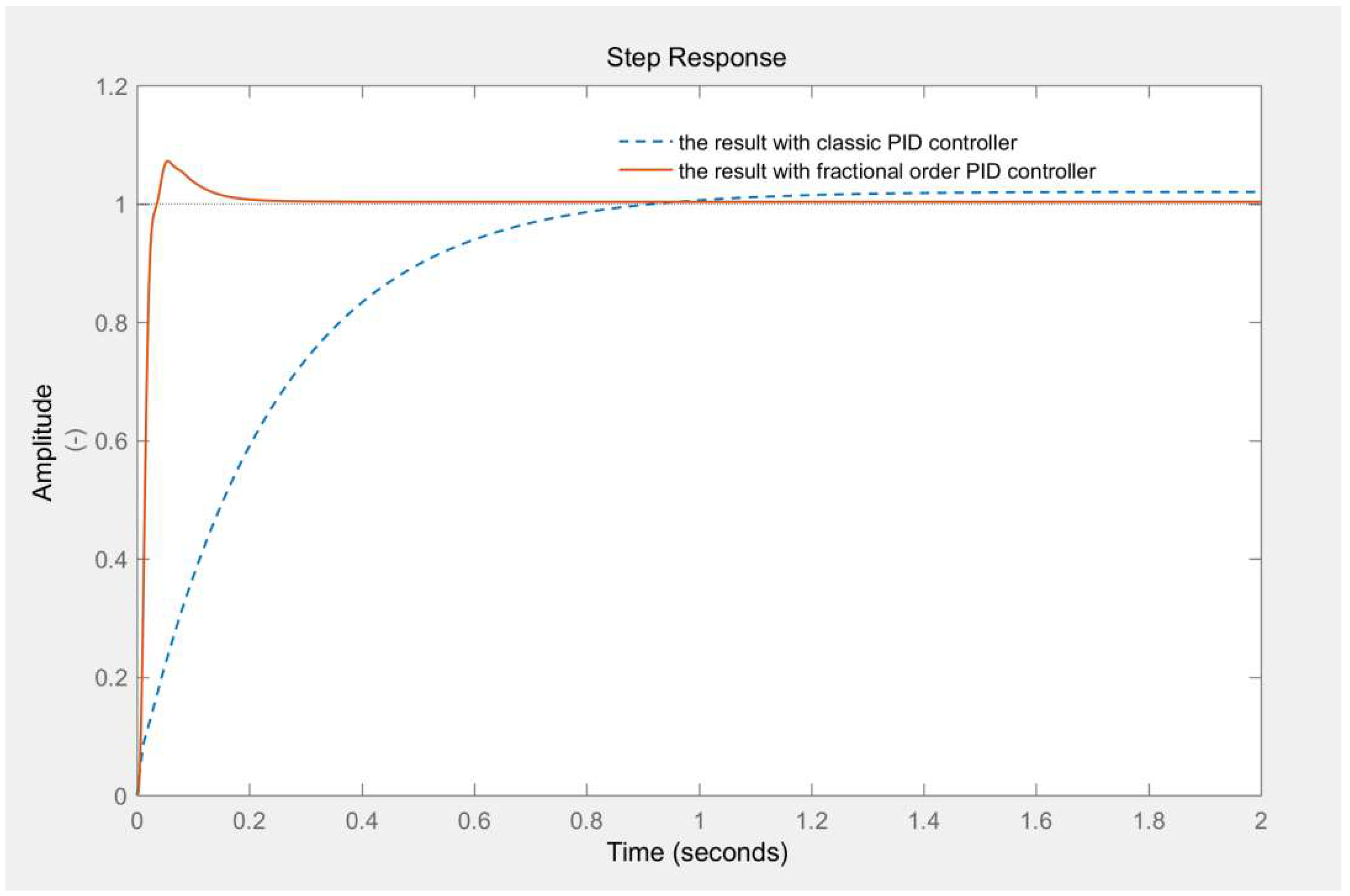
In contrast to classical PID controllers, fractional-order PID controllers involve an integration degree, $\lambda$, and a differential degree, $\mu$. Fractional-order controllers can have greater flexibility for control than classical PID controllers. Fractional-order control is an extension of conventional integral-order control. Fractional-order PID control allows dynamic properties of the fractional-order system to be adjusted to a greater extent.

The output of the fractional-order PID control in the temporal field can be shown:

$$u(t)=K_{P}e(t)+K_I{D}^{-\lambda }e(t)+K_D{D}^{\mu }e(t)$$

(12)

Here, $K_P$ denotes proportion gaining. $K_I$ represents an integration constant, and $K_D$ indicates a differential constant. The symbols $\lambda$ and $\mu$ denote the fractional degree. If $\lambda =1$ with $\mu =1$, a conventional integral-order PID controller will be received. When $\lambda =1$ with $\mu =0$, the result becomes a PI control. When $\lambda =0$ with $\mu =1$, the result becomes a PD control. When $\lambda =0$ with $\mu =0$, this is the gain. All these classical kinds of PID converters serve particular situations for fractional-order PID converters. The relationship between fractional-order PID control and PID control is a very important issue. The relations ought to be fully verified. The verification provides a basis for the wide application of fractional-order PID control. The relationship between fractional-order PID control with conventional integral-order PID control is based on the relationship between fractional-order calculus and conventional integral-order calculus, and the formalization of this relationship extends the range of applicability of credible fractional-order systematic certification, with verification increasing the reliability of a fractional-order system. Fractional-order PID control is formally analyzed in this section. On the basis of the fractional-order calculus GL definition, a formalized pattern of the fractional-order PID controller is structured in HOL.

Definition 3.

Fractional-Order PID controller

|-!Lambda Mu K_P K_I K_D e_tt.u_t Lambda Mu K_P K_I K_D e_t t =

  K_P * e_t t + K_I * frac_cal e_t (-Lambda) 0 t t

   + K_D * frac_cal e_t Mu 0 t t

Here, u_t denotesan operator export signal. e_t representsa controller input sign. The Lambdaand Muindicate an integral order anda differential order. The K_P, K_I, and K_D denote proportiongaining, integration constant, and derivative constant, separately.

Some related properties for fractional-order PID control can be formally verified based on the fractional-order properties. The higher-order logical theorems are shown below.

Theorem 5.

FRAC_PID_CLASSIC_PID

|- 0 < t /\ (Lambda = 1) /\ (Mu = 1) /\

  frac_cal_exists e_t 1 0 t t/\deriv_exists e_t t ==>

    (u_t Lambda Mu K_P K_I K_D e_t t = K_P * e_t t +

      K_I * integral (0,t) e_t t + K_D * deriv e_t t)

Theorem 6.

FRAC_PID_PI

|- 0 < t/\ (Lambda = 1)/\ (Mu = 0) ==>

  (u_t Lambda Mu K_P K_I K_D e_t t = (K_P + K_D) * e_t t

    + K_I * integral (0,t) e_t t)

Theorem 7.

FRAC_PID_PD

|- 0 < t/\ (Lambda = 0)/\ (Mu = 1)/\ frac_cal_exists e_t 1 0 t t

  /\ deriv_exists e_t t ==> (u_t Lambda Mu K_P K_I K_D e_t t

    = (K_P + K_I) * e_t t + K_D * deriv e_t t)

Theorem 8.

FRAC_PID_GAIN

|- 0 < t /\ (Lambda = 0) /\ (Mu = 0) ==>

  (u_t Lambda Mu K_P K_I K_D e_t t = (K_P + K_I + K_D) * e_t t)

Theorem 5 shows that fractional-order PID control becomes conventional integral-order PID control when the integration degree and differential degree become 1. Theorem 6 states that fractional-order PID control becomes conventional PI control when the integral order is 1 and the differential order is 0. Theorem 7 shows that fractional-order PID control becomes conventional PD control when the integration degree is 0 and the differentiation degree is 1. Theorem 8 proposes that fractional-order PID control becomes a gain if the integral order and differential order are 0. The proof process passes mainly based on the relationship between fractional-order calculus with conventional integral-order calculus.

During the formalization of these theorems, many prerequisite features were verified in HOL. These prerequisites ensure the establishment of theorems. The frac_cal_exists and derive_exists functions guarantee the existence of fractional-order calculus and traditional differentiation.

These verifications also involve large reasoning efforts based on real number theory. They spent approximately 1500 rows of HOL coding and around 30 work hours. The formalization of fractional-order PID control can ensure the completeness of the control system.

4.3. Formalization of the Fractional-Order Closed-Loop System

A fractional-order system may be described in terms of a fractional-order differential equation with n terms:

$$a_n{D}^{{\beta }_n}y(t)+a_{n-1}{D}^{{\beta }_{n-1}}y(t)+\cdots +a_0{D}^{{\beta }_0}y(t)=u(t)$$

(13)

In the above formula, $D^{\beta }={}^{0}D{}_t^{\beta }$, $a_i(i=0,1,\cdots ,n)$ is an arbitrary constant, ${\beta }_j(j=0,1,\cdots ,n)$ is an arbitrary real number, and ${\beta }_n>{\beta }_{n-1}>\cdots >{\beta }_1>{\beta }_0\ge 0$.

The higher-order logic model of the fractional-order system is constructed using the higher-order logic definition frac_cal from fractional-order calculus and the sum of the summation function. In HOL, the model is as follows:

Definition 4.

Formalization of the fractional-order system

|- FRAC_ORDER_SYSTEM <=> !n p a y u t.0 <= p 0/\

 (!j. j < n ==> p j < p (SUC j))

    ==>(sum (0,SUC n) (\i. a i * frac_cal y (p i) 0 t t) = u t)

The formalization of Definition 4 is the basis of the mathematical model for fractional-order differential equations. In the formalization process, the constants and order of Equation (13) have a subscript. To facilitate the formalization, the idea of the function is used in the definition. The $a(i)$ of Definition 4 represents the $a_i$ of Equation (13). $a(i)$ is a function in which the variable is i and the type is num-> real. $p(j)$ represents the ${\beta }_j$ of Equation (13). $p(j)$ is also a function in which the variable is j and the type is num-> real. Here, to meet the HOL idea that all symbols can be played using a keyboard, the body of the function is written as p instead of $\beta$. The antecedent (!j. j < n ==> p j < p (SUC j)) satisfies the requirement that the degree of fractional-order calculus increases within the fractional-order regime.

Another common description of a fractional-order system is expressed within the frequency region. The frequent region model is called a transfer function. It is shown as follows:

$$G_f(s)=\frac{Y(s)}{u(t)}=\frac{1}{a_n{s}^{{\beta }_n}+a_{n-1}{s}^{{\beta }_{n-1}}+\cdots +a_0{s}^{{\beta }_0}}$$

(14)

The time domain model and the frequency domain model are equivalent and can be transformed into each other. Laplace transform is required for the conversion of the time domain and frequency domain. Therefore, we first construct the formal model of the Laplace transform.

Definition 5.

Laplace transforms

|-!s g t. LAPLACE s g t = lim(\n.lim(\b.integral (1/2 pow n,&b)

  (\t. g t * exp (-(s * t))) t))

Laplace transform is defined as an integration in the integration interval $\left[0,\infty \right]$, with the integrand function being the product of g(t) and $e^{-st}$. The lim is the seeking limit, and the integral is a quadrature. The Laplace transform is a conversion of the system between the temporal region with frequent region. In order to formally verify the fractional-order controller, this paper introduces fractional-order Laplace transform. The formal expression of fractional-order Laplace transformation can be constructed in the following:

Definition 6.

Fractional-OrderLaplace transformation

|- FRAC_LAPLACE <=> !F s g t v.(F s = LAPLACE s g t) ==>

  (s rpow v * F s = frac_cal g v 0 t t)

The definition of fractional-order Laplace transformation allows the transformation of fractional-order models to lie between the temporal region and frequent region. The condition F s = LAPLACE sgt satisfies the requirement that the fractional-order Laplace transformation function g(t) must satisfy the relevant conditions of traditional Laplace transformation. g(t) represents the function before the transformation. F(s) represents the function after the transform. frac_cal represents the formalized definition of fractional-order calculus.

Fractional-order PID transfer function can be obtained through Laplace transform. Its formalization in HOL:

Theorem 9.

FRAC_PID_TD_FD

|- 0 < s/\ 0 < E s/\ FRAC_LAPLACE/\ (LAPLACE s u t = U s)

 /\ (LAPLACE s e t = E s)/\ (u t = u_t Lambda Mu K_P K_I K_D e_t t)

  ==>(U s/E s = K_P + K_I * s rpow -Lambda + K_D * s rpow Mu)

Here, the antecedents LAPLACE sut = U s and LAPLACE set = E s satisfy the requirement that the import function e(t), with the output function u(t) of the controller, satisfy the Laplace transform. Then, the fractional-order Laplace transform’s formalized definition, FRAC_LAPLACE, is applied to deduce the fractional-order Laplace transform of e(t) and u(t). Finally, the fractional-order PID control transfer function could be induced as K_P + K_I*s rpow–Lambda + K_D*s rpow Mu. In the verification, the main process includes:

g ‘(0<s)/\(0 < E(s))/\ FRAC_LAPLACE/\(LAPLACE s u = U(s))/\(LAPLACE s e = E(s))/\ (u t = u_t Lambda Mu K_P K_I K_D e t) ==>

(U(s)/E(s) = K_P + K_I * s rpow (-Lambda) + K_D * s rpow Mu)‘;

e (DISCH_TAC THEN ONCE_ASM_REWRITE_TAC [] THEN POP_ASSUM K_TAC);

e(KNOW_TAC(--‘!(v:real).frac_cal e v 0 t t = s rpow v * E(s)‘--));

e(GEN_TAC);

e(ONCE_REWRITE_TAC[FRAC_LAPLACE]);

e(REPEAT STRIP_TAC);

e(POP_ASSUM MP_TAC);

e(RW_TAC real_ss[REAL_MUL_ASSOC]).

The following theorem verifies the equivalence of the fractional-order time domain model and the frequency domain model based on the Laplace transform.

Theorem 10.

FRAC_ORDER_SYSTEM_TD_FD

|-0 < s/\ (!i. 0 < a i)/\ U s <> 0/\(LAPLACE s u t = U s)

 /\ (LAPLACE s y t = Y s) /\FRAC_LAPLACE/\ FRAC_ORDER_SYSTEM

   ==>(Y s/U s = 1/sum (0,SUC n) (\i. a i * s rpow p i))

Theorem 10 proves that the time domain of fractional-order systems can be transformed to the corresponding transfer function through the Laplace transform. The antecedent U s<> 0 satisfies the requirement that U(s) is not equal to zero. The antecedents 0 < sand !i. 0 < a(i) can deduce that the requirement sum (0,SUC n) (\i. a i * s rpow p i)) is not equal to zero. Therefore, they can perform a divisor. Under these conditions, the FRAC_ORDER_SYSTEM can be expressed as 1/sum (0,SUC n) (\i. a i * s rpow p i). In the verification, the main process includes:

e(REPEAT STRIP_TAC);

e(POP_ASSUM MP_TAC);

e(ONCE_REWRITE_TAC[FRAC_LAPLACE]);

e(KNOW_TAC(--‘!(i:num).a(i) *frac_cal y (p i) 0 t t = a(i) * s rpow (p i) * Y(s)‘--));

e(GEN_TAC);

e(RW_TAC real_ss[REAL_EQ_LMUL2]);

e (DISCH_TAC THEN ONCE_ASM_REWRITE_TAC [] THEN POP_ASSUM K_TAC);

e(CONV_TAC SYM_CONV);

e(KNOW_TAC(--‘Y s * inv (U s) * sum (0,SUC n) (\i. a i * s rpow p i) = Y s * sum (0,SUC n) (\i. a i * s rpow p i) * inv (U s)‘--));

e(CONV_TAC(AC_CONV(REAL_MUL_ASSOC,REAL_MUL_COMM))).

Here, fractional-order closed-loop systems may be formalized through the transfer functions of fractional-order PID and fractional-order systems. The corresponding mathematical model is as follows:

$$G_S(s)=\frac{G_f(s)G_c(s)}{1+G_f(s)G_c(s)}$$

(15)

The fractional-order closed-loop system’s corresponding higher-order logic model can be shown as follows:

Definition 7.

Fractional-Orderclosed-loop system

|-!a p n Lambda Mu K_P K_I K_D s.G_s a p n Lambda Mu K_P K_I K_D s

= G_f a p s n * G_c Lambda Mu K_P K_I K_D s/

  (1 + G_f a p s n * G_c Lambda Mu K_P K_I K_D s)

In Definition 7, G_f, G_c, G_s, respectively, represent the transfer functions of fractional-order control objective, fractional-order PID, and fractional-order closed-loop system. G_s can be obtained through G_f and G_c. To facilitate the application of this, this paper generalizes the definition of fractional-order closed-loop systems. The formalization is shown by the following:

Theorem 11.

CL_LO_SYS_TRANSFER_GENERAL

|-!n a s p K_P K_D K_I Lambda Mu. 0 < s/\ (!i. 0 < a i)

 /\ u_t Lambda Mu K_P K_I K_D e_t t <> 0 ==>

 (G_s a p n Lambda Mu K_P K_I K_D s = (K_D * s rpow (Lambda + Mu)

   + K_P * s rpow Lambda + K_I)/(sum (0,SUC n)

     (\i. a i * s rpow (p i + Lambda)) +

      K_D * s rpow (Lambda + Mu) + K_P * s rpow Lambda + K_I))

• where Lambda and Mu denote the integrationdegreewith differentiationdegree. K_P, K_I, and K_D represent the proportion gaining, integration coefficient, and differentiation coefficient, respectively. s indicates a transfer functionfor the variables. The antecedents 0 < s and (!i. 0 < a i) can induce the sum (0,SUC n) (\i. a i * s rpow p i) as not being equal zero. Then,that s rpow Lambda * sum (0,SUC n) (\i. a i * s rpow p i) is not equal to zero can be provenaccording to the fact thats rpow Lambda is greater than zero. That (1 + 1/sum (0,SUC n) (\i. a i * s rpow p i) * (K_P + K_I * s rpow -Lambda + K_D * s rpow Mu)) is not equal to zero can be inducedby the fact that the transfer function of the controlsystem u_t Lambda Mu K_P K_I K_D e_t t is not equal to zero. In the verification, the main process includes:

e(RW_TAC real_ss[FRAC_ORDER_SYSTEM_TRANSFER,FRAC_PID_TRANSFER]);

e(MATCH_MP_TAC REAL_DIV_MUL2);

e (DISCH_TAC THEN ONCE_ASM_REWRITE_TAC [] THEN POP_ASSUM K_TAC);

e(KNOW_TAC(--‘(s rpow Lambda * sum (0,SUC n) (\i. a i * s rpow p i) * (1/sum (0,SUC n) (\i. a i * s rpow p i) * (K_P + K_I * s rpow -Lambda + K_D * s rpow Mu))) = (s rpow Lambda * (K_P + K_I * s rpow -Lambda + K_D * s rpow Mu))‘--));

e(ONCE_REWRITE_TAC[GSYM REAL_MUL_ASSOC]);

e(ONCE_ASM_REWRITE_TAC[]).

Some mathematical operations must follow higher-order logic and be derived according to the existing theorem in HOL. Therefore, in the induction process, the equation needs to transfer the form of the existing theorem and rewrite the theorem. Having the sub-goals turn into the form of the existing theorem is a more complicated matter. Because the turning needs to meet the formal structure of HOL, and this also reflects the rigor of HOL. As with the above division, that the denominator is not zero must be given or proven. If these antecedents are not given, using related theorems of division cannot rewrite the goals.

This theorem is the formalized verification of the general form for fractional-order closed-loop systems. It may be the basic model for a fractional-order closed-loop control system. This lays a foundation for the formalized verification of a fractional-order closed-loop control system. The following specifically verifies the stability of the fractional-order system.

5. Higher-Order Logic Verification

The stability of fractional-order PID control for the fractional-order bottom control systems of robots can be formalized on the basis of the characters and theorems in HOL. The formal analyses of the fractional-order system consist of two parts: the modeling of higher-order logic and its verification.

The steady-state output of a robot’s fractional-order control system is verified when the input is the unit step response. In HOL, the unit step response is formalized as follows:

Definition 8.

Unit step response

|-!x. unit x = if 0 < x then 1 else 0

Some basic theorems of fractional-order calculus, such as the fractional-order differential of a constant, are also required for the verification of fractional-order systems. This paper defines a fractional-order differential of a constant as one where the result is zero, like the integer-order differential of the constant. Its formalized model can be established by the following:

Definition 9

. Fractional-order differential of a constant

|- FRAC_CAL_CONST <=> !v t c. 0 < v/\

  (frac_cal (\t. c) v 0 t t = 0)

Through inverse fractional-order Laplace transformation, the output of the time domain for the fractional-order system designed above, may be obtained by the following:

$$y(t)=\frac{6.58D^{0.8}u(t)+7.99D^{0.2}u(t)+20.915}{0.00001196D^{3.2}u(t)+0.002404D^{2.2}u(t)+0.7523D^{1.2}u(t)+6.58D^{0.8}u(t)+7.99D^{0.2}u(t)+20.915}$$

(16)

On the basis of the established formalized pattern, the steady state of the fractional-order system is verified. The formalized form can be established and verified on account of the time model of the fractional-order control system as follows:

Theorem 12.

POSITION_SERVO_SYSTEM_UNIT

|- ∀t.0<t/\ FRAC_CAL_CONST ==>

 ((6.58 * frac_cal (\t. unit t) 0.8 0 t t +

  7.99 * frac_cal (\t. unit t)0.2 0 t t + 20.915)/

   (0.00001196 * frac_cal (\t. unit t) 3.2 0 t t +

    0.002404 * frac_cal (\t. unit t) 2.2 0 t t +

     0.7523 * frac_cal (\t. unit t) 1.2 0 t t +

    6.58 * frac_cal (\t. unit t) 0.8 0 t t +

      7.99 * frac_cal (\t. unit t) 0.2 0 t t + 20.915) = 1)

The stability of the robot controlled by the fractional-order PID can be verified using the above theorem. Here, frac_cal denotes the formalized definition of fractional-order calculus. FRAC_CAL_CONST stands for the equation that the fractional-order calculus of a constant is 0, namely, ${}_{0}D{}_t^{\alpha }C=0$. Here, C is a constant. $\alpha$ stands for a fractional degree, and represents an actual number larger than 0. The system input unit is a unit-step response, which is a jump function with a value of 1 when time t is greater than 0. The antecedent of theorem t is greater than 0 and is determined by the current system, which guarantees that the unit-step response will be 1. After this, the conclusion, that, in terms of the property that the fractional-order calculus of a constant becomes zero, is drawn. The stability of the theorem is expressed as 1 and the conclusion that the theorem holds will be automatically drawn when the left side of the equation of the theorem is calculated to be 1. The result of the proof is shown in Figure 2, which is that the fractional-order control system has a steady state output. In the verification, the main process includes:

e(RW_TAC real_ss[]);

e(KNOW_TAC(--‘(frac_cal (\t. unit t) 0.8 0 t t = 0)‘--));

e(FULL_SIMP_TAC real_ss[FRAC_CAL_UNIT]);

e (ONCE_ASM_REWRITE_TAC [] THEN POP_ASSUM K_TAC);

e (POP_ASSUM K_TAC).

The reliability verification of the controlling scheme shows the effectiveness and potentiality of fractional-order PID control designed in this paper. The verification of this property also demonstrates that the theory proof based on higher-order logic may formally verify the control system of robots. And this also offers a firm theoretical grounding for the research and development of fractional-order control systems.

6. Conclusions

Increasingly, robots are becoming part of our daily life. The safety and reliability of these robot systems are of vital importance. Thus, robot manipulation technology is gaining increasing interest. In the article, we construct the fractional-order PID control with higher reliability for underlying robotic control systems. The superiority of fractional-order PID control was gained through simulation. Then, the fractional-order PID control was verified by higher-order logic. The higher-order logic formal verification method has completeness and can ensure precision and security for robot fractional-order PID systems. The relationship between fractional-order calculus and integral-order calculus was formalized. Those features may be applied to build and verify safety-critical fractional-order PID control for HOL. Formalizations of fractional-order PID control systems provide the foundations for the formalized analyses of fractional-order families. The stability of fractional-order PID control is verified in HOL. And the formal method also offers a theoretical basis for fractional-order schemes.