A Fractional Model of Complex Permittivity of Conductor Media with Relaxation: Theory vs. Experiments

Abstract

Moving from the study of plasmonic materials with relaxation, in this work we propose a fractional Abraham–Lorentz-like model of the complex permittivity of conductor media. This model extends the Ciancio–Kluitenberg, based on the Mazur–de Groot non-equilibrium thermodynamics theory (NET). The approach based on NET allows us to link the phenomenological function of internal variables and electrodynamics variables for a large range of frequencies. This allows us to closer reproduce experimental data for some key metals, such as Cu, Au and Ag. Particularly, our fitting significantly improves those obtained by Rakic and coworkers and we were able to operate in a larger range of energy values. Moreover, in this work we also provide a definition of a substantial fractional derivative, and we extend the fractional model proposed by Flora et al.

1. Introduction

The electromagnetic behavior of materials is characterized by the electric and magnetic permittivities. The actual mechanisms that determine this behavior are due to the action of the forces that interact on the system resulting in dissipative phenomena involving a large number of microscopic units and a nontrivial dynamics of entropy production. As such, these phenomena can be usefully described by non-equilibrium thermodynamics (NET). In particular, the theoretical apparatus proposed by De Groot and Mazur [1,2] is of particular interest when investigating dynamic irreversible phenomena. Remarkably, they introduced the concept of internal variables. to model internal dissipative phenomena at a macroscopic scale. In the framework of the NET [1,2,3], by extending the works [4,5,6,7,8,9], Ciancio and Flora [10] proposed a fractional model of dielectric permittivity that is more general than the key models of the literature.

As far as metals [11] are concerned, existing fractional models such as [12], although providing useful insights, are limited by a short range of wavelengths and do not focus on energy adsorption and scattering.

Given the above-illustrated framework, here we introduce a new fractional model of relaxation for conductors. Our aim is to show that this new approach is able to perform better than previous models inferred from quantum mechanics, such as [13]. Moreover, this improvement is obtained both in a larger number of material and in larger ranges of energies. We also aim at (i) improving the inference of the surface plasmonic waves; (ii) improving the inference of the scattered fields by conductors. This work is organized as follows: in Section 2, we summarize relevant research of interest; in Section 3, we infer the fractional substantial derivative, which we later utilize; in Section 4, we extend the fractional dielectric model of [10]; in Section 5, we apply our framework to plasmonic materials with relaxation; in Section 6, we propose a new model for media conductors, which employs classical derivatives; in Section 7, we propose a fractional model for conductors; in Section 8, we show our result and comparisons with other models. This work is ended by general conclusions, illustrated in Section 9.

2. Survey of the Ciancio–Kluitenberg Theory of Dielectric Media with Relaxation

In order to set a framework for our study, in this section we briefly summarize papers [4,5], where dielectric and magnetic relaxation phenomena are discussed in the framework of the general theory of de Groot and Mazur NET. Interested readers with a more mathematical background are recommended to read the books [1,2] and the long review [14] on non-equilibrium thermodynamical phenomena, and books [15,16,17] on electromagnetic theory and applications.

In those works, it was shown that a vector internal variable that influences the polarization gives rise to dielectric relaxation phenomena. If one linearizes this theory and neglects cross-effects due to electric conduction, heat conduction and viscosity on electric relaxation, the following relaxation equation may be obtained:

$${\chi }_{\left(EP\right)}^{\left(0\right)}\mathbf{E}+\frac{d\mathbf{E}}{dt}={\chi }_{\left(PE\right)}^{\left(0\right)}\mathbf{P}+{\chi }_{\left(PE\right)}^{\left(1\right)}\frac{d\mathbf{P}}{dt}+{\chi }_{\left(PE\right)}^{\left(2\right)}\frac{d^2\mathbf{P}}{d{t}^2}$$

(1)

where ${\chi }_{\left(EP\right)}^{\left(0\right)}$, ${\chi }_{\left(PE\right)}^{\left(0\right)}$, ${\chi }_{\left(PE\right)}^{\left(1\right)}$ and ${\chi }_{\left(PE\right)}^{\left(2\right)}$ are algebraic functions of the coefficients occurring in the phenomenological equations and in the equations of state. The relaxation equation represents a balance between the changes of the electric field $\mathbf{E}$ and those of the electrical polarization $\mathbf{P}$, caused by irreversible processes that are associated to diffusion as well as to electric and thermal conduction; the operator $d/dt$ denotes the substantial derivative, useful in the case where the mean is not immobile;

$$\mathbf{E}(\mathbf{x},t)={[E_1(\mathbf{x},t),E_2(\mathbf{x},t),E_3(\mathbf{x},t)]}^T;$$

$$\mathbf{P}(\mathbf{x},t)={[P_1(\mathbf{x},t),P_2(\mathbf{x},t),P_3(\mathbf{x},t)]}^T;$$

$$\mathbf{x}={[x_1,x_2,x_3]}^T;$$

$${\chi }_{\left(EP\right)}^{\left(0\right)}=a_{\left(P\right)}^{(1,1)}{L}_{\left(P\right)}^{(1,1)};$$

(2)

$${\chi }_{\left(PE\right)}^{\left(0\right)}=a_{\left(P\right)}^{(0,0)}\left[a_{\left(P\right)}^{(1,1)}-a_{\left(P\right)}^{(0,0)}\right]L_{\left(P\right)}^{(1,1)};$$

(3)

$${\chi }_{\left(PE\right)}^{\left(1\right)}=a_{\left(P\right)}^{(0,0)}\left[1+L_{\left(P\right)}^{(0,1)}-L_{\left(P\right)}^{(1,0)}\right]+a_{\left(P\right)}^{(1,1)}\left[L_{\left(P\right)}^{(0,0)}{L}_{\left(P\right)}^{(1,1)}-L_{\left(P\right)}^{(0,1)}{L}_{\left(P\right)}^{(1,0)}\right];$$

(4)

$${\chi }_{\left(EP\right)}^{\left(2\right)}=L_{\left(P\right)}^{(0,0)};$$

(5)

and where $L_{\left(P\right)}^{(0,0)}$, $L_{\left(P\right)}^{(0,1)}$, $L_{\left(P\right)}^{(1,0)}$, $L_{\left(P\right)}^{(1,1)}$ are the phenomenological coefficients and $a_{\left(P\right)}^{(0,0)}$ , $a_{\left(P\right)}^{(1,1)}$ are scalar constants.

Ciancio–Kluitenberg’s Ordinary Dielectric Model (CK-O)

In this subsection, we summarize the main features of the Ciancio–Kluitenberg’s ordinary dielectric model (CK-O). Let $\mathbf{D}$ be the electrical induction and ${ϵ}_0$ be the dielectric constant in the void, replacing the constitutive equation of $\mathbf{P}$:

$$\mathbf{P}=\mathbf{D}-{ϵ}_0\mathbf{E}$$

(6)

in the (1), with ${\chi }_{PE}^{\left(2\right)}\ne 0$, we obtain:

$${ϵ}_0\left\{\frac{d^2}{d{t}^2}\mathbf{E}+\frac{\left(1+{ϵ}_0\right){\chi }_{PE}^{\left(1\right)}}{{ϵ}_0{\chi }_{PE}^{\left(2\right)}}\frac{d}{dt}\mathbf{E}+\frac{\left[{\chi }_{\left(EP\right)}^{\left(0\right)}+{\chi }_{\left(PE\right)}^{\left(0\right)}\right]}{{ϵ}_0{\chi }_{PE}^{\left(2\right)}}\mathbf{E}\right\}=\frac{d^2}{d{t}^2}\mathbf{D}+\frac{{\chi }_{\left(PE\right)}^{\left(1\right)}}{{\chi }_{PE}^{\left(2\right)}}\frac{d}{dt}\mathbf{D}+\frac{{\chi }_{\left(PE\right)}^{\left(0\right)}}{{\chi }_{PE}^{\left(2\right)}}\mathbf{D}$$

(7)

Setting:

$${\chi }_{\left(ED\right)}^{\left(0\right)}={\chi }_{\left(EP\right)}^{\left(0\right)}+{\chi }_{\left(PE\right)}^{\left(0\right)}$$

(8)

$${\chi }_{\left(ED\right)}^{\left(1\right)}=\left(1+{ϵ}_0\right){\chi }_{\left(PE\right)}^{\left(1\right)}$$

(9)

$${\chi }_{\left(DE\right)}^{\left(0\right)}={\chi }_{\left(PE\right)}^{\left(0\right)}$$

(10)

$${\chi }_{\left(DE\right)}^{\left(1\right)}={\chi }_{\left(PE\right)}^{\left(1\right)}$$

(11)

$${\chi }^{\left(2\right)}={\chi }_{\left(PE\right)}^{\left(2\right)}$$

(12)

one obtains the CK-O’s model:

$${ϵ}_0{\chi }^{\left(2\right)}\frac{d^2}{d{t}^2}\mathbf{E}+{\chi }_{\left(ED\right)}^{\left(1\right)}\frac{d}{dt}\mathbf{E}+{\chi }_{\left(ED\right)}^{\left(0\right)}\mathbf{E}={\chi }^{\left(2\right)}\frac{d^2}{d{t}^2}\mathbf{D}+{\chi }_{\left(DE\right)}^{\left(1\right)}\frac{d}{dt}\mathbf{D}+{\chi }_{\left(DE\right)}^{\left(0\right)}\mathbf{D}$$

(13)

3. Inference of the Fractional Substantial Derivative

In this section, we infer the fractional substantial derivative. This is a mathematical tool that is useful for the determination of the distribution of vector fields in a fractional space. We employ it in order to obtain an analytical formula for the computation of the complex permittivity.

In the unidimensional case, the substantial derivative of a (scalar or vectorial) field reads as follows:

$$\frac{d}{dt}\varphi (x,t)=v{\partial }_x\varphi (x,t)+{\partial }_t\varphi (x,t)$$

(14)

There are many definitions of fractional derivative [18] (see Appendix A). We adopted the Caputo derivative, since we believe that it well suits the problems related to high-frequency electromagnetic fields. Indeed, the Caputo fractional derivative has a kernel particularly fit to describe the surface propagation of polarons; a second and important reason: the Caputo fractional derivative [19] is particularly fit to describe phenomena with memory [20]. Fractional derivatives based on non-singular kernels would not be appropriate. Apart from the above-mentioned reasons, we think (and results seems to agree with our vision) that the use of the Caputo derivative in the model allows a better phenomenological of the behavior of plasmonic media. In particular, the association to the inter-band interplay electron–electron, electron–phonon and in the surface scattering can be easily described without recurring to a full quantum description. Thus, the use of a fractional approach allowed us to better fit experimental data. In the framework of Caputo fractional calculus [19], the partial derivatives of a field reads as follows

$${}^C{\partial }_t^{\left(\alpha \right)}\varphi (x,t)=\frac{1}{\mathrm{\Gamma }(1-\alpha )}{\int }_0^t\frac{{\partial }_{\tau }\varphi (x,\tau )}{{(t-\tau )}^{\alpha }}d\tau$$

(15)

$${}^C{\partial }_x^{\left(\alpha \right)}\varphi (x,t)=\frac{1}{\mathrm{\Gamma }(1-\alpha )}{\int }_0^x\frac{{\partial }_{\xi }\varphi (\xi ,t)}{{(\xi -x)}^{\alpha }}d\xi$$

(16)

where $\alpha$ is an order non-integer of the fractional derivative, $\mathrm{\Gamma }(1-\alpha )$ is Euler Gamma function, ${(t-\tau )}^{-\alpha }$ is the fractional temporal kernel and ${(\xi -x)}^{-\alpha }$ is the fractional spatial kernel. Spherical coordinates are useful from a computational point of view, for example, to determine the differential equation of the scalar potential that solves the problem of the field absorbed and scattered by a spherical particle of metal [21]. In this section, we report a new expression of substantial derivative that depends on the metric of fractional space and on the position of a material point with respect to a system of spherical coordinates.

Let us consider a plane wave propagating in an isotropic space. In this case, the fractional order depends only on the propagation direction found by the unitary vector ${\widehat{\mathbf{u}}}_r$. It is shown that if $v=0$ then the substantial fractional derivative coincides with the partial derivative relative to time.

3.1. Distance of a Material Point from the Origin

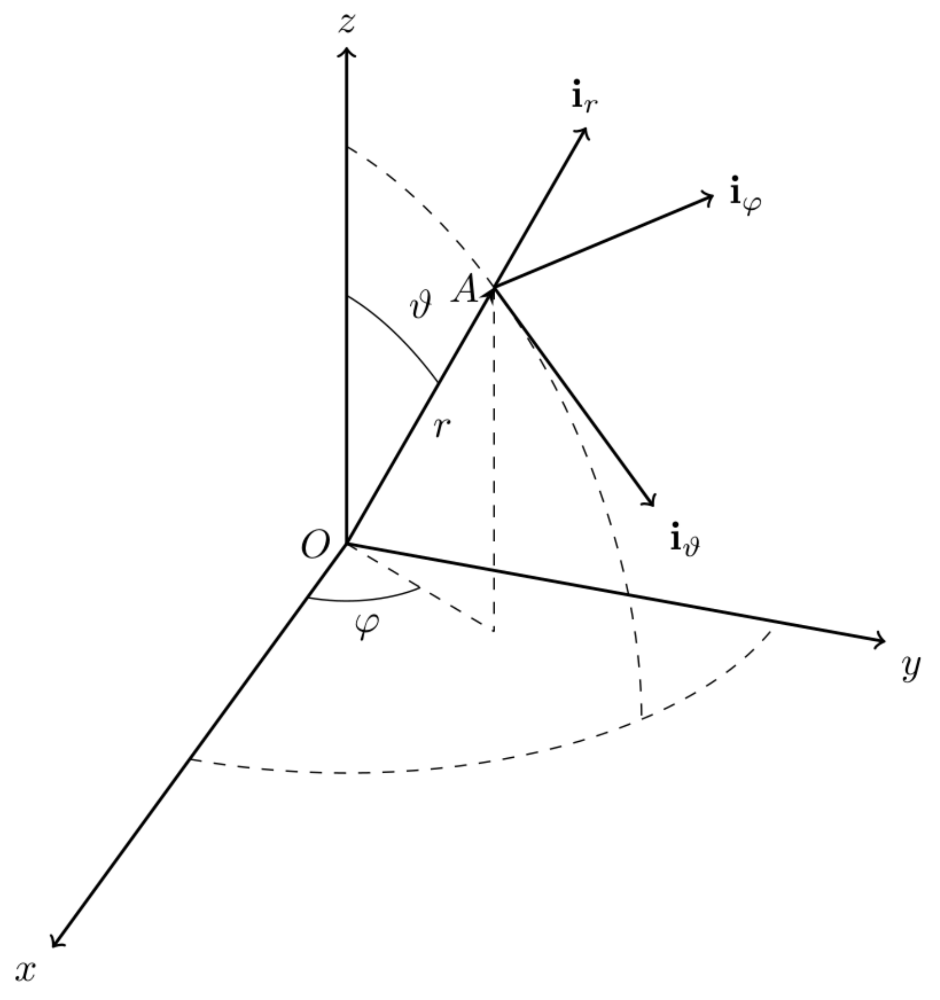
The concept of metric intervenes in geometry whenever it becomes necessary to measure certain geometric entities that belong to a given space. For example, the distance of a point from the origin, the area of a surface, etc... In a fractional space, we calculate the distance of an object placed in point A from the origin of a reference system in spherical coordinates, Figure 1, by means the fractional integral of Caputo.

The Caputo integral of a $f\left(r\right)$ function is given by:

$${\displaystyle I_r^{\alpha }\left[f\left(r\right)\right]=\frac{1}{\mathrm{\Gamma }\left(\alpha \right)}{\int }_0^{r}f\left(r\right){(r-\xi )}^{\alpha -1}d\xi }$$

Using spherical coordinates, the distance of a point in the position r with respect to the origin is given by:

$${\displaystyle I_r^{\alpha }\left[1\right]=\frac{1}{\mathrm{\Gamma }\left(\alpha \right)}{\int }_0^r{(r-\xi )}^{\alpha -1}d\xi }$$

(17)

The integral is immediate (17). Setting:

$$\zeta =r-\xi$$

we have:

$$d\zeta =-d\xi$$

$$\xi =0\Rightarrow \zeta =r$$

$$\xi =x\Rightarrow \zeta =0$$

therefore the (17) becomes:

$${\displaystyle I_r^{\alpha }\left[1\right]=-\frac{1}{\mathrm{\Gamma }\left(\alpha \right)}{\int }_r^0{\zeta }^{\alpha -1}d\zeta =\frac{1}{\mathrm{\Gamma }\left(\alpha \right)}{\int }_0^r{\zeta }^{\alpha -1}d\zeta }$$

(18)

i.e.,

$${\displaystyle {}^C{l}^{\left(\alpha \right)}\left(r\right)=I_r^{\alpha }\left[1\right]=\frac{r^{\alpha }}{\mathrm{\Gamma }(1+\alpha )}}$$

(19)

representing the distance, in fractional space, of point P in the position r with respect to the origin of a reference system in spherical coordinates [22]. If $\alpha =1$ we observe: $\mathrm{\Gamma }(n+1)=n!$, with $n\in \mathcal{N}$, then: $\mathrm{\Gamma }(\alpha +1)=\mathrm{\Gamma }\left(2\right)=1$.

3.2. The Substantial Fractional Derivative of Caputo

From the definition of a substantial ordinary derivative of a vector function $\mathbf{V}(r,t)$:

$${\displaystyle \frac{d\mathbf{V}(r,t)}{dt}={\partial }_t\mathbf{V}(r,t)+{\partial }_r\mathbf{V}(r,t)\frac{dr}{dt}}$$

The fractional derivative of Caputo is:

$${\displaystyle {}^C{\mathfrak{D}}_t^{{}^{\left(\alpha \right)}}\left[\mathbf{V}(r,t)\right]=\frac{1}{\mathrm{\Gamma }(1-\alpha )}{\int }_0^t\frac{{\displaystyle \frac{d\mathbf{V}\left(r,\tau \right)}{d\tau }}}{{(t-\tau )}^{\alpha }}d\tau }$$

(20)

Applying the equation to the expression of the ordinary substantive derivative, replacing the ’classical’ partial derivative with the partial fractional derivative and taking into account the metric yields:

$${}^C{\mathfrak{D}}_t^{{}^{\left(\alpha \right)}}\left[\mathbf{V}(r,t)\right]={}^C{\partial }_t^{{}^{\left(\alpha \right)}}\mathbf{V}(r,t)+{}^C{\partial }_r^{{}^{\left(\alpha \right)}}\mathbf{V}(r,t){}^C{\mathfrak{D}}_t^{{}^{\left(\alpha \right)}}\left[{\displaystyle \frac{r^{\alpha }}{\mathrm{\Gamma }(1+\alpha )}}\right]$$

(21)

where the fractional partial derivatives with respect to t and s are given, respectively, from (15) and (16), with:

$${\displaystyle {}^C{\mathfrak{D}}_t^{{}^{\left(\alpha \right)}}\left[r^{\alpha }\right]=\frac{1}{\mathrm{\Gamma }\left(\alpha \right)\mathrm{\Gamma }(1-\alpha )}{\int }_0^t\frac{r^{\alpha -1}v\left(\tau \right)}{{(t-\tau )}^{\alpha }}d\tau }$$

(22)

From the (21) and (15), (16) and (22), the substantial fractional derivative is:

$${\displaystyle {}^C{\mathfrak{D}}_t^{{}^{\left(\alpha \right)}}\left[\mathbf{V}(r,t)\right]=\frac{1}{\mathrm{\Gamma }(1-\alpha )}{\int }_0^t\frac{{\partial }_t\mathbf{V}\left(r,\tau \right)}{{(t-\tau )}^{\alpha }}d\tau +\frac{1}{\mathrm{\Gamma }\left(\alpha \right)\mathrm{\Gamma }(1-\alpha )}{\int }_0^t\frac{r^{\alpha -1}v\left(\tau \right)}{{(t-\tau )}^{\alpha }}d\tau {\int }_0^r\frac{{\partial }_{\xi }\mathbf{V}\left(\xi ,t\right)}{{(r-\xi )}^{\alpha }}d\xi }$$

(23)

In the particular case where $v\left(\tau \right)=const.$, we have:

$$r=vt$$

i.e.,:

$${\displaystyle {\int }_0^t\frac{r^{\alpha -1}v\left(\tau \right)}{{(t-\tau )}^{\alpha }}d\tau =v^{\alpha }{t}^{\alpha -1}{\int }_0^t\frac{1}{{(t-\tau )}^{\alpha }}d\tau ={\int }_0^t\frac{r^{\alpha -1}v\left(\tau \right)}{{(t-\tau )}^{\alpha }}d\tau =v^{\alpha }{t}^{\alpha -1}{t}^{1-\alpha }=v^{\alpha }}$$

$${\displaystyle {}^C{\mathfrak{D}}_t^{{}^{\left(\alpha \right)}}\left[\mathbf{V}(r,t)\right]=\frac{1}{\mathrm{\Gamma }(1-\alpha )}{\int }_0^t\frac{{\partial }_t\mathbf{V}\left(r,\tau \right)}{{(t-\tau )}^{\alpha }}d\tau +\frac{v^{\alpha }}{\mathrm{\Gamma }\left(\alpha \right)\mathrm{\Gamma }(1-\alpha )}{\int }_0^r\frac{{\partial }_{\xi }\mathbf{V}\left(\xi ,t\right)}{{(r-\xi )}^{\alpha }}d\xi }$$

(24)

Finally, if $v=0$ the substantial fractional derivative coincides with the partial fractional derivative respect to t, expressed by the (15). In the case of $v\left(\tau \right)=const.$, the complete Laplace transform of the (24) is:

$$L{T}_{r}L{T}_t\left\{{}^C{\mathfrak{D}}_t^{{}^{\left(\alpha \right)}}\left[\mathbf{V}(r,t)\right]\right\}=\left({\displaystyle s^{\alpha }+\frac{{\left(vk\right)}^{\alpha }}{\mathrm{\Gamma }\left(\alpha \right)}}\right)\widehat{\mathbf{V}}\left(k,s\right)$$

(25)

4. Extending the Ciancio–Kluitenberg’s Fractional Dielectric Model (CK-F)

The above illustrated Ciancio–Kluitenberg theory for dielectrics was developed by using classical derivatives. Here, we aim at widening its scope by employing fractional derivatives.

We assume that the electromagnetic field is represented by means of plane electromagnetic waves propagating along $x_1$. Putting:

$${\displaystyle A_1=\frac{a_1}{a_2};A_0=\frac{a_0}{a_2};C_1=\frac{c_1}{c_2};C_0=\frac{c_0}{c_2}}$$

where:

$$a_2={ϵ}_0{\chi }^{\left(2\right)}$$

$$a_1={\chi }_{\left(ED\right)}^{\left(1\right)}$$

$$a_0={\chi }_{\left(ED\right)}^{\left(0\right)}$$

$$c_2={\chi }^{\left(2\right)}$$

$$c_1={\chi }_{\left(DE\right)}^{\left(1\right)}$$

$$c_0={\chi }_{\left(DE\right)}^{\left(0\right)}$$

Substituting the ordinary substantial derivative in the equation with the fractional substantial derivative (21) implied that the (13) becomes:

$${ϵ}_0\left({}^C{\mathfrak{D}}_t^{{}^{\left(2\alpha \right)}}\mathbf{E}+A_1{}^C{\mathfrak{D}}_t^{{}^{\left(\alpha \right)}}\mathbf{E}+A_0\mathbf{E}\right)={}^C{\mathfrak{D}}_t^{{}^{\left(2\alpha \right)}}\mathbf{D}+C_1{}^C{\mathfrak{D}}_t^{{}^{\left(\alpha \right)}}\mathbf{D}+C_0\mathbf{D}$$

(26)

with: $\mathbf{E}=\mathbf{E}(x_1,t)$ and $\mathbf{D}=\mathbf{D}(x_1,t)$.

By moving the two-dimensional Laplace transformation to both sides, we obtain the CK-F’s model in the Laplace domain $(0,k,s)$:

$${ϵ}_0\left({\xi }_2(k,s)+A_1{\xi }_1(k,s)+A_0)\right)\widehat{\mathbf{E}}(k,s)=\left({\xi }_2(k,s)+C_1{\xi }_1(k,s)+C_0\right)\widehat{\mathbf{D}}(k,s)$$

(27)

where:

$$\widehat{\mathbf{E}}(k,s)={\int }_0^{+\infty }{\int }_0^{+\infty }\mathbf{E}(x_1,t)exp(-k{x}_1)exp(-st)d{x}_{1}dt$$

(28)

$$\widehat{\mathbf{D}}(k,s)={\int }_0^{+\infty }{\int }_0^{+\infty }\mathbf{D}(x_1,t)exp(-k{x}_1)exp(-st)d{x}_{1}dt$$

(29)

$${\xi }_2(k,s)={(s+vk)}^{2\alpha }$$

(30)

$${\xi }_1(k,s)={(s+vk)}^{\alpha }$$

(31)

with: $s=\Re \left(s\right)+i\omega$.

If the reference system is fixed, i.e., $v=0$, the substantial derivative shall be equal to the Eulerian derivative:

$$v=0⟺{}^C{\mathfrak{D}}_t^{{}^{\left(\alpha \right)}}\left(·\right)={}^C{\partial }_t^{{}^{\left(\alpha \right)}}\left(·\right)$$

(32)

and in the case $\Re \left(s\right)=0$, one has:

$${\xi }_2\left(\omega \right)={\left(i\omega \right)}^{2\alpha }$$

(33)

$${\xi }_1\left(\omega \right)={\left(i\omega \right)}^{\alpha }$$

(34)

Therefore Equation (27) becomes:

$${ϵ}_0\left({\left(i\omega \right)}^{2\alpha }+A_1{\left(i\omega \right)}^{\alpha }+A_0)\right)\mathbf{E}(k,\omega )=\left({\left(i\omega \right)}^{2\alpha }+C_1{\left(i\omega \right)}^{\alpha }+C_0\right)\mathbf{D}(k,\omega )$$

(35)

According to the constitutive equation:

$$\mathbf{D}(k,\omega )=ϵ(\omega ;\alpha )\mathbf{E}(k,\omega )$$

(36)

by (35), one has:

$$ϵ(\omega ;\alpha )={ϵ}_0\frac{{\left(i\omega \right)}^{2\alpha }+A_1{\left(i\omega \right)}^{\alpha }+A_0}{{\left(i\omega \right)}^{2\alpha }+C_1{\left(i\omega \right)}^{\alpha }+C_0}$$

(37)

representing the fractional permittivity of order $\alpha$.

5. Plasmonic Materials with Relaxation

As we have seen in Section 2, the De Groot and Mazur NET theory has been applied to dielectric media with memory in [3,5,23,24]. This was performed through the link between internal variables and phenomenological coefficients, and allowed us to derive an analytical representation of electromagnetic properties and, in particular, the complex permittivity and the wave vector of the electromagnetic field. The above theory, in agreement with the second principle of thermodynamics, leads to a relaxation equation of the general form (see formula (1.3) [25]):

$${\chi }_{\left(EP\right)}^{\left(0\right)}\mathbf{E}+{\chi }_{\left(EP\right)}^{\left(1\right)}\frac{d\mathbf{E}}{dt}+\cdots +\frac{d^n\mathbf{E}}{d{t}^n}={\chi }_{\left(PE\right)}^{\left(0\right)}\mathbf{P}+{\chi }_{\left(PE\right)}^{\left(1\right)}\frac{d\mathbf{P}}{dt}+\cdots +{\chi }_{\left(PE\right)}^{(n+1)}\frac{d^{(n+1)}\mathbf{P}}{d{t}^{(n+1)}}.$$

(38)

The above equation may be extended in the case of plasmonic materials, through internal variables and associated phenomenological coefficients, if the following conditions are met:

• The electric field $\mathbf{E}$ trend depends only on the polarization $\mathbf{P}$ and the instantaneous variations of $\mathbf{P}$.
• The polarization induced by the incident electromagnetic field generates a radiant field that opposes the inelastic behavior due to interactions near the surface of the metal, at the microscopic level, to electron–electron, electron–phonon and electron–surface scattering. This apparent field source produces a radiant reaction force ${\mathbf{F}}_{rad}$, (see formula (11.80) in [16]) proportional to the instantaneous derivative of the third order of polarization due to the concentration of free electrons near the surface:

  $${\mathbf{F}}_{rad}\propto \frac{d^3\mathbf{r}}{d{t}^3}$$

  being:

  $$\mathbf{P}=Nq\mathbf{r}$$

  where N is the concentration of electrons and q the electric charge, it follows that:

  $${\mathbf{F}}_{rad}\propto \frac{d^3\mathbf{P}}{d{t}^3}$$
  As a result, instantaneous changes of the polarization that are above the third order can be overlooked.

The first condition implies that:

$${\chi }_{{}_{\left(EP\right)}}^{\left(1\right)}\frac{d\mathbf{E}}{dt}+{\chi }_{{}_{\left(EP\right)}}^{\left(2\right)}\frac{d^2\mathbf{E}}{d{t}^2}+\cdots +{\chi }_{{}_{\left(EP\right)}}^{(n-1)}\frac{d^{n-1}\mathbf{E}}{d{t}^{n-1}}+\frac{d^n\mathbf{E}}{d{t}^n}=0$$

(39)

that replaced in (38) gives:

$${\chi }_{\left(EP\right)}^{\left(0\right)}\mathbf{E}={\chi }_{\left(PE\right)}^{\left(0\right)}\mathbf{P}+{\chi }_{\left(PE\right)}^{\left(1\right)}\frac{d\mathbf{P}}{dt}+{\chi }_{\left(PE\right)}^{\left(2\right)}\frac{d^2\mathbf{P}}{d{t}^2}+\cdots +{\chi }_{\left(PE\right)}^{(n+1)}\frac{d^{(n+1)}\mathbf{P}}{d{t}^{(n+1)}}$$

(40)

If the above conditions are met, the general relaxation Equation (38) in the case of perfectly conductive materials becomes:

$${\chi }_{\left(EP\right)}^{\left(0\right)}\mathbf{E}={\chi }_{\left(PE\right)}^{\left(0\right)}\mathbf{P}+{\chi }_{\left(PE\right)}^{\left(1\right)}\frac{d\mathbf{P}}{dt}+{\chi }_{\left(PE\right)}^{\left(2\right)}\frac{d^2\mathbf{P}}{d{t}^2}+{\chi }_{\left(PE\right)}^{\left(3\right)}\frac{d^3\mathbf{P}}{d{t}^3}$$

(41)

6. A New Ordinary Derivatives-Based Model for Conductors

Thanks to the new concepts introduced in Section 5, we are able now to develop a new model applicable to conductors and based on classical derivatives.

Transforming both members of the (41) with respect to time, since the $\mathbf{E}$ field moves away from the conductor, we have:

$$\mathbf{P}(k,\omega )=\frac{{\chi }_{\left(EP\right)}^{\left(0\right)}}{\left({\chi }_{\left(PE\right)}^{\left(0\right)}-{\chi }_{\left(PE\right)}^{\left(2\right)}{\omega }^2\right)-i\omega \left({\chi }_{\left(PE\right)}^{\left(1\right)}-{\chi }_{\left(PE\right)}^{\left(3\right)}{\omega }^2\right)}\mathbf{E}(k,\omega )$$

(42)

Applying Fourier transform to Equation (6) yields:

$$\mathbf{P}(k,\omega )=\mathbf{D}(k,\omega )-{ϵ}_0\mathbf{E}(k,\omega )=\left(ϵ-{ϵ}_0\right)\mathbf{E}(k,\omega )$$

(43)

from the comparison of (42) with the (43) we obtain the ordinary Ciancio–Kluitenberg model that represents the complex relative permittivity of the conductive media:

$$ϵ={ϵ}_0\left(1-\frac{{\displaystyle \frac{{\chi }_{\left(EP\right)}^{\left(0\right)}}{{ϵ}_0{\chi }_{\left(PE\right)}^{\left(2\right)}}}}{\left({\displaystyle {\omega }^2-\frac{{\chi }_{\left(PE\right)}^{\left(0\right)}}{{\chi }_{\left(PE\right)}^{\left(2\right)}}}\right)+i\omega \left({\displaystyle \frac{{\chi }_{\left(PE\right)}^{\left(1\right)}}{{\chi }_{\left(PE\right)}^{\left(2\right)}}-\frac{{\chi }_{\left(PE\right)}^{\left(3\right)}}{{\chi }_{\left(PE\right)}^{\left(2\right)}}{\omega }^2}\right)}\right)$$

(44)

If we impose:

$${\displaystyle {\omega }_p^2=\frac{{\chi }_{\left(EP\right)}^{\left(0\right)}}{{ϵ}_0{\chi }_{\left(PE\right)}^{\left(2\right)}};{\omega }_0^2=\frac{{\chi }_{\left(PE\right)}^{\left(0\right)}}{{\chi }_{\left(PE\right)}^{\left(2\right)}};\mathrm{\Gamma }=\frac{{\chi }_{\left(PE\right)}^{\left(1\right)}}{{\chi }_{\left(PE\right)}^{\left(2\right)}};\frac{{\mathrm{\Gamma }}_s}{m_e}=\frac{{\chi }_{\left(PE\right)}^{\left(3\right)}}{{\chi }_{\left(PE\right)}^{\left(2\right)}}}$$

(45)

then we obtain the Abraham–Lorentz model [26]

$$ϵ={ϵ}_0\left(1-\frac{{\omega }_p^2}{\left({\omega }^2-{\omega }_0^2\right)+i\omega \left({\displaystyle \mathrm{\Gamma }-\frac{{\mathrm{\Gamma }}_s}{m_e}{\omega }^2}\right)}\right)$$

(46)

where $\mathrm{\Gamma }$ is damping factor, ${\omega }_p$ is plasmon pulsation, ${\omega }_0$ is pulsation of the natural oscillation, $m_e$ is mass of the electron and ${\displaystyle {\mathrm{\Gamma }}_s=\frac{q^2}{6\pi {ϵ}_0{c}^3}}$ is the damping factor component due to the radiation reaction, which depends on the square of the angular pulsation. This formulation has previously been derived, in another way, by using the concept of radiation reaction force, which contradicts Newton’s third principle as discussed in [16]. The theory of NET overcomes this contradiction.

If the coefficient ${\chi }_{\left(PE\right)}^{\left(3\right)}=0$, i.e., the radiation reaction is not considered, the Drude–Lorentz model is obtained:

$$ϵ={ϵ}_0\left(1-\frac{{\displaystyle \frac{{\chi }_{\left(EP\right)}^{\left(0\right)}}{{ϵ}_0{\chi }_{\left(PE\right)}^{\left(2\right)}}}}{\left({\displaystyle {\omega }^2-\frac{{\chi }_{\left(PE\right)}^{\left(0\right)}}{{\chi }_{\left(PE\right)}^{\left(2\right)}}}\right)+i\omega \left({\displaystyle \frac{{\chi }_{\left(PE\right)}^{\left(1\right)}}{{\chi }_{\left(PE\right)}^{\left(2\right)}}}\right)}\right)$$

(47)

that is, for the first three relations of the (45):

$$ϵ={ϵ}_0\left(1-\frac{{\omega }_p^2}{\left({\omega }^2-{\omega }_0^2\right)+i\omega \mathrm{\Gamma }}\right)$$

(48)

which represents the Drude–Lorentz model in the form obtained by another way in [17]. If the natural oscillation pulsation (${\omega }_0$) is negligible, we obtain the Drude model.

7. A Fractional Conductor Model

Here we change paradigm by employing fractional derivatives in our model.

Considering the fractional differential equation corresponding to the (41), substituting the ordinary derivative for the fractional one, we obtain the fractional relaxation equation for plasmonic materials:

$${\chi }_{\left(EP\right)}^{\left(0\right)}\mathbf{E}={\chi }_{\left(PE\right)}^{\left(0\right)}\mathbf{P}+{\chi }_{\left(PE\right)}^{\left(1\right)}{}^C{\mathfrak{D}}_t^{{}^{\left(\alpha \right)}}\mathbf{P}+{\chi }_{\left(PE\right)}^{\left(2\right)}{}^C{\mathfrak{D}}_t^{{}^{\left(2\alpha \right)}}\mathbf{P}+{\chi }_{\left(PE\right)}^{\left(3\right)}{}^C{\mathfrak{D}}_t^{{}^{\left(3\alpha \right)}}\mathbf{P}$$

(49)

Applying the properties of the Laplace transform and keeping in mind that the $\mathbf{E}$ field moves away from the conductor, we immediately obtain the Ciancio–Kluitenberg’s fractional model expression of the relative complex permittivity to the media perfectly conductive:

$$ϵ={ϵ}_0+\frac{{\displaystyle \frac{{\chi }_{\left(EP\right)}^{\left(0\right)}}{{\chi }_{\left(PE\right)}^{\left(2\right)}}}}{{\displaystyle {\left(i\omega \right)}^{2\alpha }+\frac{{\chi }_{\left(PE\right)}^{\left(0\right)}}{{\chi }_{\left(PE\right)}^{\left(2\right)}}-{\left(i\omega \right)}^{\alpha }\left({\displaystyle \frac{{\chi }_{\left(PE\right)}^{\left(1\right)}}{{\chi }_{\left(PE\right)}^{\left(2\right)}}+\frac{{\chi }_{\left(PE\right)}^{\left(3\right)}}{{\chi }_{\left(PE\right)}^{\left(2\right)}}{\left(i\omega \right)}^{2\alpha }}\right)}}$$

(50)

The electromagnetic behavior of conductors depends on quantum phenomena and atomic interactions, such as those between electron–electron and electron–phonon, whose description is very complex. Applying the theory of the joint density of states, the resulting models has more than 30 variable parameters, whose determination is difficult and laborious (see [13]). An alternative semi-quantum theory, describing the behavior of conductor materials, has been formulated in [27,28].

The fractional order of the derivative allows to determine the values of algebraic functions that, within the fixed limits of the considered interval and taking into account the increase in entropy, gives a good approximation of the relative complex permittivity. To describe phenomena that occur on electronic scale (from ${10}^{15}@{10}^{18}$ Hz) the system must be represented by a system of m fractional relaxation equations, where m depends on the material. The first Equation (51) describes intra-band interaction while the remaining $m-1$ equations describe inter-band transitions:

$${\chi }_{\left(EP\right)}^{(0,0)}\mathbf{E}={\chi }_{\left(PE\right)}^{(1,0)}{}^C{\mathfrak{D}}_t^{{}^{\left({\alpha }_0\right)}}\mathbf{P}+{\chi }_{\left(PE\right)}^{(2,0)}{}^C{\mathfrak{D}}_t^{{}^{\left(2{\alpha }_0\right)}}\mathbf{P}$$

(51)

$${\chi }_{\left(EP\right)}^{(0,1)}\mathbf{E}={\chi }_{\left(PE\right)}^{(0,1)}\mathbf{P}+{\chi }_{\left(PE\right)}^{(1,1)}{}^C{\mathfrak{D}}_t^{{}^{\left({\alpha }_1\right)}}\mathbf{P}+{\chi }_{\left(PE\right)}^{(2,1)}{}^C{\mathfrak{D}}_t^{{}^{\left(2{\alpha }_1\right)}}\mathbf{P}+{\chi }_{\left(PE\right)}^{(3,1)}{}^C{\mathfrak{D}}_t^{{}^{\left(3{\alpha }_1\right)}}\mathbf{P}$$

(52)

$$\begin{gathered} \cdots \\ {\chi }_{\left(EP\right)}^{(0,q)}\mathbf{E}={\chi }_{\left(PE\right)}^{(0,q)}\mathbf{P}+{\chi }_{\left(PE\right)}^{(1,q)}{}^C{\mathfrak{D}}_t^{{}^{\left({\alpha }_q\right)}}\mathbf{P}+{\chi }_{\left(PE\right)}^{(2,q)}{}^C{\mathfrak{D}}_t^{{}^{\left(2{\alpha }_q\right)}}\mathbf{P}+{\chi }_{\left(PE\right)}^{(3,q)}{}^C{\mathfrak{D}}_t^{{}^{\left(3{\alpha }_q\right)}}\mathbf{P} \\ \cdots \end{gathered}$$

(53)

$${\chi }_{\left(EP\right)}^{(0,m-1)}\mathbf{E}={\chi }_{\left(PE\right)}^{(0,m-1)}\mathbf{P}+{\chi }_{\left(PE\right)}^{(1,m-1)}{}^C{\mathfrak{D}}_t^{{}^{\left({\alpha }_{m-1}\right)}}\mathbf{P}+{\chi }_{\left(PE\right)}^{(2,m-1)}{}^C{\mathfrak{D}}_t^{{}^{\left(2{\alpha }_{m-1}\right)}}\mathbf{P}+{\chi }_{\left(PE\right)}^{(3,m-1)}{}^C{\mathfrak{D}}_t^{{}^{\left(3{\alpha }_{m-1}\right)}}\mathbf{P}$$

(54)

Applying the Fourier transform to the above equations, we easily obtain the complex relative permittivity:

$${ϵ}_r^{AL}(\omega ,T)={ϵ}_{r_{Intraband}}^{AL}(\omega ,T)+{ϵ}_{r_{Interband}}^{AL}(\omega ,T)$$

(55)

where:

$${\displaystyle {ϵ}_{r_{Intraband}}^{AL}(\omega ,T)=1+\frac{f_0{\omega }_p^2}{{\left(i\omega \right)}^{2{\alpha }_0}-{\left(i\omega \right)}^{{\alpha }_0}({\tilde{\mathrm{\Gamma }}}_0+{\left(i\omega \right)}^{2{\alpha }_0}{\mathrm{\Gamma }}_{0,s})}}$$

(56)

$${ϵ}_{r_{Interband}}^{AL}(\omega ,T)=\sum _{q=1}^{m-1}\frac{f_q{\omega }_p^2}{{\left(i\omega \right)}^{2{\alpha }_q}+{\omega }_q^{2{\alpha }_q}-{\left(i\omega \right)}^{{\alpha }_q}\left({\mathrm{\Gamma }}_q+{\left(i\omega \right)}^{2{\alpha }_q}{\mathrm{\Gamma }}_{q,s}\right)}$$

(57)

where ${\omega }_q$ is the pulsation of the natural oscillation. Note that the phenomenological coefficients associated with the state variables represent the physical quantities of a system consisting of oscillators characterized by their own elastic mass proportional to the plasmon pulsation ${\omega }_p$ of the material, from a damping factor ${\mathrm{\Gamma }}_q$ and a resonant frequency ${\omega }_q$, with $q=1,2,...,m-1$. The damping factor, ${\tilde{\mathrm{\Gamma }}}_0$, depends on electron–electron, electron–phonon and surface scattering:

$${\tilde{\mathrm{\Gamma }}}_0={\mathrm{\Gamma }}_0+\mathrm{\Gamma }\left(T\right)-\mathrm{\Gamma }\left(T_0\right)$$

(58)

where $T_0=293.15$ K is the room temperature. Taking:

$${\alpha }_0=1$$

the term $f_0{\omega }_p^2$ may be seen as the square of an effective plasmonic angular frequency ${\mathsf{\Omega }}_p(T;\gamma )$:

$${\mathsf{\Omega }}_p^2(T;\gamma )=\frac{f_0{\omega }_p^2}{1+3\gamma (T-T_0)}$$

(59)

where $\gamma$ volumetric expansion coefficient of the metal that for gold is equal to $14.2\times {10}^{-6}{\mathrm{K}}^{-1}$.

The intra-band damping factor, $\mathrm{\Gamma }\left(T\right)$, is given by:

$$\mathrm{\Gamma }\left(T\right)={\mathrm{\Gamma }}_{e-e}+{\mathrm{\Gamma }}_{e-ph}+{\mathrm{\Gamma }}_{Surf}$$

(60)

where:

$${\mathrm{\Gamma }}_{e-e}\left(T\right)=\frac{{\pi }^3\mathsf{\Phi }\Delta }{12\hslash E_F}\left[{\left(K_{B}T\right)}^2+{\left(\frac{\hslash \omega }{2\pi }\right)}^2\right]$$

(61)

for gold (Au): $\mathsf{\Phi }=0.55$; $\Delta =0.77$; $E_F=5.5$[eV]; $K_B\approx 1.381\times {10}^{-23}\left[\mathrm{J}\right]{\left[\mathrm{T}\right]}^{-1}$, where $E_F$ is Fermi’s level.

$${\mathrm{\Gamma }}_{e-ph}\left(T\right)={\mathrm{\Gamma }}_{ib}\left[\frac{2}{5}+\frac{4T^5}{{\Theta }_D^5}{\int }_0^{{\Theta }_D/T}\left(\frac{z^4}{e^z-1}\right)dz\right]$$

(62)

for Au: ${\mathrm{\Gamma }}_{ib}=0.07$[eV]; ${\Theta }_D=170$[K]

$${\mathrm{\Gamma }}_{Surf}=\frac{A{v}_f}{L_{eff}}$$

(63)

with: ${\displaystyle L_{eff}=\frac{4V}{S}}$. The DL model is obtained by canceling the damping factor due to the Abraham–Lorentz force:

$${\displaystyle {ϵ}_r^{DL}(\omega ,T)=1+\frac{f_0{\omega }_p^2}{{\left(i\omega \right)}^{2{\alpha }_0}-{\left(i\omega \right)}^{{\alpha }_0}{\tilde{\mathrm{\Gamma }}}_0}+\sum _{q=1}^{m-1}\frac{f_q{\omega }_p^2}{{\left(i\omega \right)}^{2{\alpha }_q}+{\omega }_q^{2{\alpha }_q}-{\left(i\omega \right)}^{{\alpha }_q}{\mathrm{\Gamma }}_q}}$$

(64)

8. Results

In this section, we validate our model. Namely, here we report the results of our simulations related to the fractional models of Drude–Lorentz and Abraham–Lorentz and we compare them with the ordinary model of Drude–Lorentz obtained by Rakic [29]. We assume that the parameters vary slowly with temperature.

Table 1. Nomenclature of the model parameters.

Parameters	Description
${\alpha }_i$	Order fractional derivative non integer
$f_i$	Strength oscillator
${\omega }_p$	Plasmon pulsation
${\omega }_i$	Pulsation of the natural oscillation
${\mathrm{\Gamma }}_i$	Damping factor
${\mathrm{\Gamma }}_{i,s}$	Damping factor due to Abraham’s radiation reaction

defines the nomenclature of the model parameters:

The proposed Abraham–Lorentz fractional model (55), considered a system with $m=6$ equations, is characterized by 30 parameters:

$${\theta }_{AL}={[f_i,b_i,{\mathrm{\Gamma }}_i,{\mathrm{\Gamma }}_{i,s},{\alpha }_i]}_{i=0}^{i=5}$$

and ${\omega }_p$, since:

$$b_0=0$$

The Drude–Lorentz fractional model, considering a system with $m=6$ equations, is characterized by 24 parameters:

$${\theta }_{DL}={[f_i,b_i,{\mathrm{\Gamma }}_i,{\alpha }_i]}_{i=0}^{i=5}$$

and ${\omega }_p$, having neglected the six parameters ${\left[{\mathrm{\Gamma }}_{i,s}\right]}_{i=0}^{i=5}$ and being:

$$b_0=0$$

The parameters of the fractional models were obtained by fitting the experimental measurements of permittivity reported in [30]. To fit these data, we used the differential evolution algorithm (DE) [31,32,33]. The DE algorithm is an iterative method of stochastic nature for the search of the possible global optimal solutions on large space of parameters. We implemented the fitting procedure by using the Python language and its scientific library scipy [34]. We have chosen the DE algorithms because of its ability to provide trustable global minima, at variance of classical deterministic optimization algorithms (such as the gradient method or Newton’s method) that are prone to stuck to local minima. Moreover, many of the deterministic algorithms additionally require to provide the derivative of the objective function. In [29,35] the SA (simulation annealing) algorithm has been used, which requires many experimental values in contrast to the DE. To compare results, unlike the original target function used:

$${\chi }^2=\sum _{\nu =1}^M{\left({\displaystyle \left|\frac{{ϵ}_{rR}\left({\omega }_{\nu }\right)-{\widehat{ϵ}}_{rR}\left({\omega }_{\nu }\right)}{{\widehat{ϵ}}_{rR}\left({\omega }_{\nu }\right)}\right|+\left|\frac{{ϵ}_{rI}\left({\omega }_{\nu }\right)-{\widehat{ϵ}}_{rI}\left({\omega }_{\nu }\right)}{{\widehat{ϵ}}_{rI}\left({\omega }_{\nu }\right)}\right|}\right)}^2$$

(65)

in this work the target functions used are:

$${\chi }_{{}_{L^2}}^2=\frac{1}{M}\sum _{\nu =1}^M\sqrt{{\displaystyle {\left({\displaystyle \frac{{ϵ}_{rR}\left({\omega }_{\nu }\right)-{\widehat{ϵ}}_{rR}\left({\omega }_{\nu }\right)}{{\widehat{ϵ}}_{rR}\left({\omega }_{\nu }\right)}}\right)}^2+{\left(\frac{{ϵ}_{rI}\left({\omega }_{\nu }\right)-{\widehat{ϵ}}_{rI}\left({\omega }_{\nu }\right)}{{\widehat{ϵ}}_{rI}\left({\omega }_{\nu }\right)}\right)}^2}}$$

(66)

and

$${\displaystyle {\chi }_{{}_{L^1}}^2=\frac{1}{M}\sum _{\nu =1}^M\left|\frac{{ϵ}_{rR}\left({\omega }_{\nu }\right)-{\widehat{ϵ}}_{rR}\left({\omega }_{\nu }\right)}{{\widehat{ϵ}}_{rR}\left({\omega }_{\nu }\right)}\right|+\left|\frac{{ϵ}_{rI}\left({\omega }_{\nu }\right)-{\widehat{ϵ}}_{rI}\left({\omega }_{\nu }\right)}{{\widehat{ϵ}}_{rI}\left({\omega }_{\nu }\right)}\right|}$$

(67)

where M is the number of experimental values related to the real part, ${\widehat{ϵ}}_{rR}\left({\omega }_{\nu }\right)$, and imaginary ${\widehat{ϵ}}_{rI}\left({\omega }_{\nu }\right)$ of the complex permittivity in function of the angular frequency $\omega$ (energy units: Electron volt). In particular, the following metals are considered: Cu, Ag and Au [30]. With reference to the experimental data on Cu, applying the DE algorithm and using the objective function given by Equation (66), in

Table 2. Parameters of the DL fractional model for copper.

i	${\mathit{\alpha }}_{\mathit{i}}$	${\mathit{f}}_{\mathit{i}}$	${\mathrm{\Gamma }}_{\mathit{i}}$	${\mathit{\omega }}_{\mathit{i}}$
0	1.004730	0.652235	0.022426	0.000000
1	2.149239	0.028789	0.305696	0.346706
2	2.292784	0.417507	0.626524	3.054485
3	1.159858	1.000000	2.563180	5.705190
4	3.096487	1.284043	1.626758	14.777767
5	0.851485	1.811348	22.872457	12.339008

and

Table 3. Parameters of the AL fractional model for copper.

i	${\mathit{\alpha }}_{\mathit{i}}$	${\mathit{f}}_{\mathit{i}}$	${{\Gamma }}_{\mathit{i}}$	${{\omega }}_{\mathit{i}}$	${\mathit{\Gamma }}_{\mathit{i},\mathit{s}}$
0	1.022008	0.810690	0.010000	0.000000	0.033524
1	2.270495	0.039793	0.299768	0.260940	0.094691
2	2.351334	0.701728	0.729006	3.434902	0.015184
3	1.333996	1.000000	1.585860	5.162526	0.118895
4	1.290008	1.484767	1.863114	9.787234	0.119947
5	0.789522	2.001560	23.401576	9.807689	0.001000

, the values of the parameters of the fractional model DL and AL are given. For the model DL, you have a ${\omega }_{p_{{}_{DL}}}=11.19$ eV , whereas for model AL you have a ${\omega }_{p_{{}_{AL}}}=10.38$ eV. We observe that the fractional order of the relaxation equation describing the intra-band component, represented by the Drude model, and the fractional orders of the relaxation equations related to the inter-band component clearly deviate from the unit. 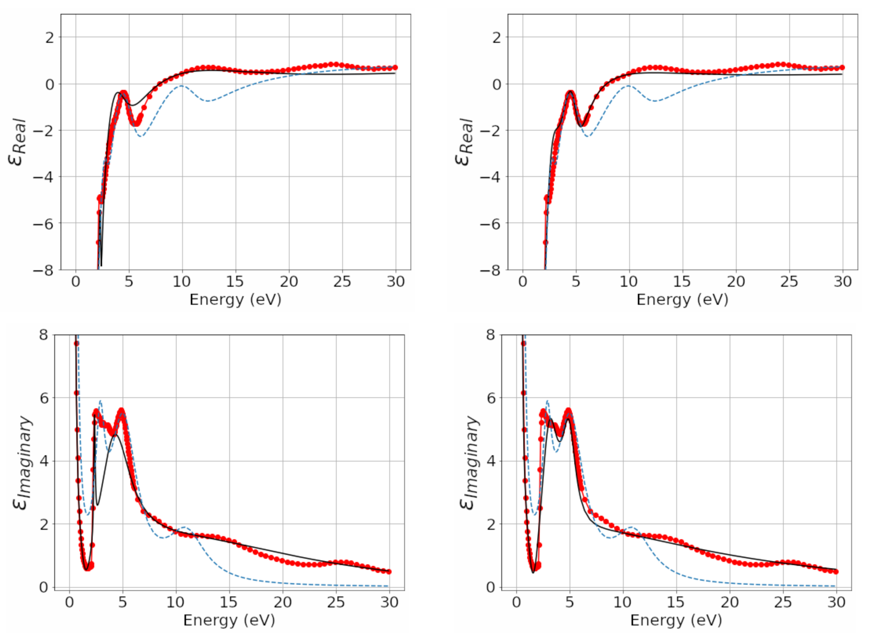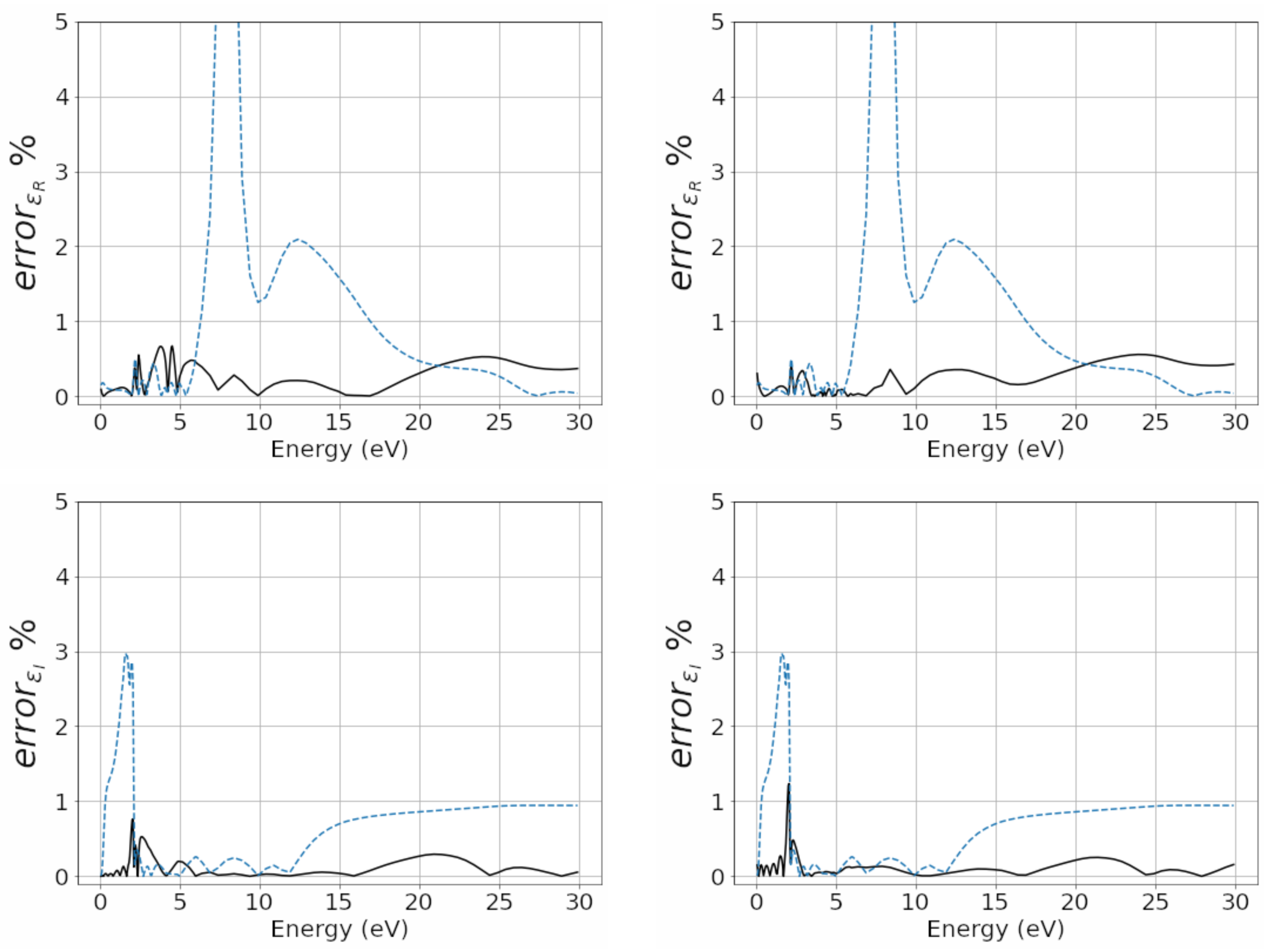In the left panels of Figure 2, the trends of the real and imaginary part of the complex permittivity, of the DL models, of Rakic and of the measurements obtained by Weaver are compared; in the left panels of the same figure, we compare the trends of the real and imaginary part of complex permittivity, models of AL, Rakic and measurements obtained by Weaver. One can observe how the AL model is better than the DL model. 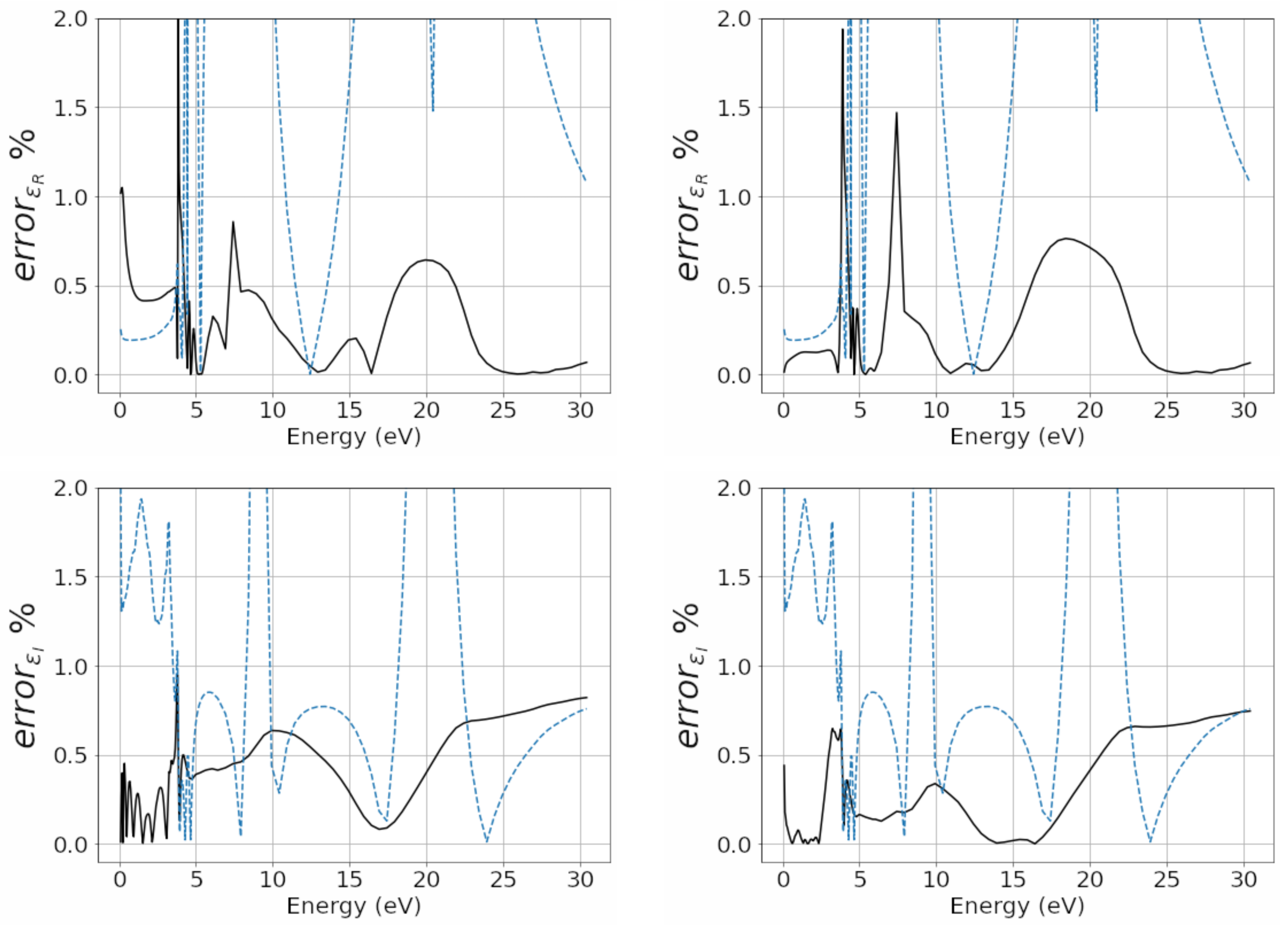In Figure 3, the relative complex permittivity errors in percent, compared to the corresponding experimental values, are reported in the left panels (upper panel the real part and lower panel the imaginary part) of the fractional models DL and Rakic; in the right panels of the same figure (upper panel the real part and lower panel the imaginary part), we report those of the models AL and Rakic. It can be observed that the trend of the relative percentage error of the DL fractional model is 1% lower for both the real and the imaginary part. The real part of the relative percentage error of the Rakic model is greater than 1% and around $7.5$ eV is more than 50%.

With reference to the experimental data on Au, applying the DE algorithm and using the objective function given by Equation (66), in

Table 4. Parameters of the DL fractional model for gold.

i	${\mathit{\alpha }}_{\mathit{i}}$	${\mathit{f}}_{\mathit{i}}$	${{\Gamma }}_{\mathit{i}}$	${\mathit{\omega }}_{\mathit{i}}$
0	1.001592	0.458696	0.051510	0.000000
1	1.534741	0.010000	0.079482	0.287249
2	0.864357	0.050155	0.715589	0.625423
3	2.729516	0.034324	0.607210	0.308078
4	1.092999	0.375837	2.293299	4.410001
5	0.974247	0.661472	2.199032	14.695663

and

Table 5. Parameters of the AL fractional model for gold.

i	${\mathit{\alpha }}_{\mathit{i}}$	${\mathit{f}}_{\mathit{i}}$	${{\Gamma }}_{\mathit{i}}$	${\mathit{\omega }}_{\mathit{i}}$	${{\Gamma }}_{\mathit{i},\mathit{s}}$
0	0.978210	0.567509	0.054493	0.000000	$0.000000\times {10}^0$
1	1.921014	0.047362	0.240568	0.055343	$9.999300\times {10}^{-7}$
2	1.314503	0.054634	0.690093	0.626431	$0.000000\times {10}^0$
3	2.928077	0.010000	0.418136	1.192927	$9.950043\times {10}^{-7}$
4	1.241883	0.833099	0.604626	4.930995	$9.993887\times {10}^{-7}$
5	1.045096	3.160085	1.057374	19.794528	$0.000000\times {10}^0$

, the values of the parameters of the fractional model DL and AL are given. For model DL, it yields ${\omega }_{p_{{}_{DL}}}=7.25$ eV, whereas for model AL you have a ${\omega }_{p_{{}_{AL}}}=8.00$ eV. It is observed how the fractional order of the relaxation equation described the intraband component, represented by the Drude model, and the fractional orders of the relaxation equations related to the interband component clearly deviate from the unit. 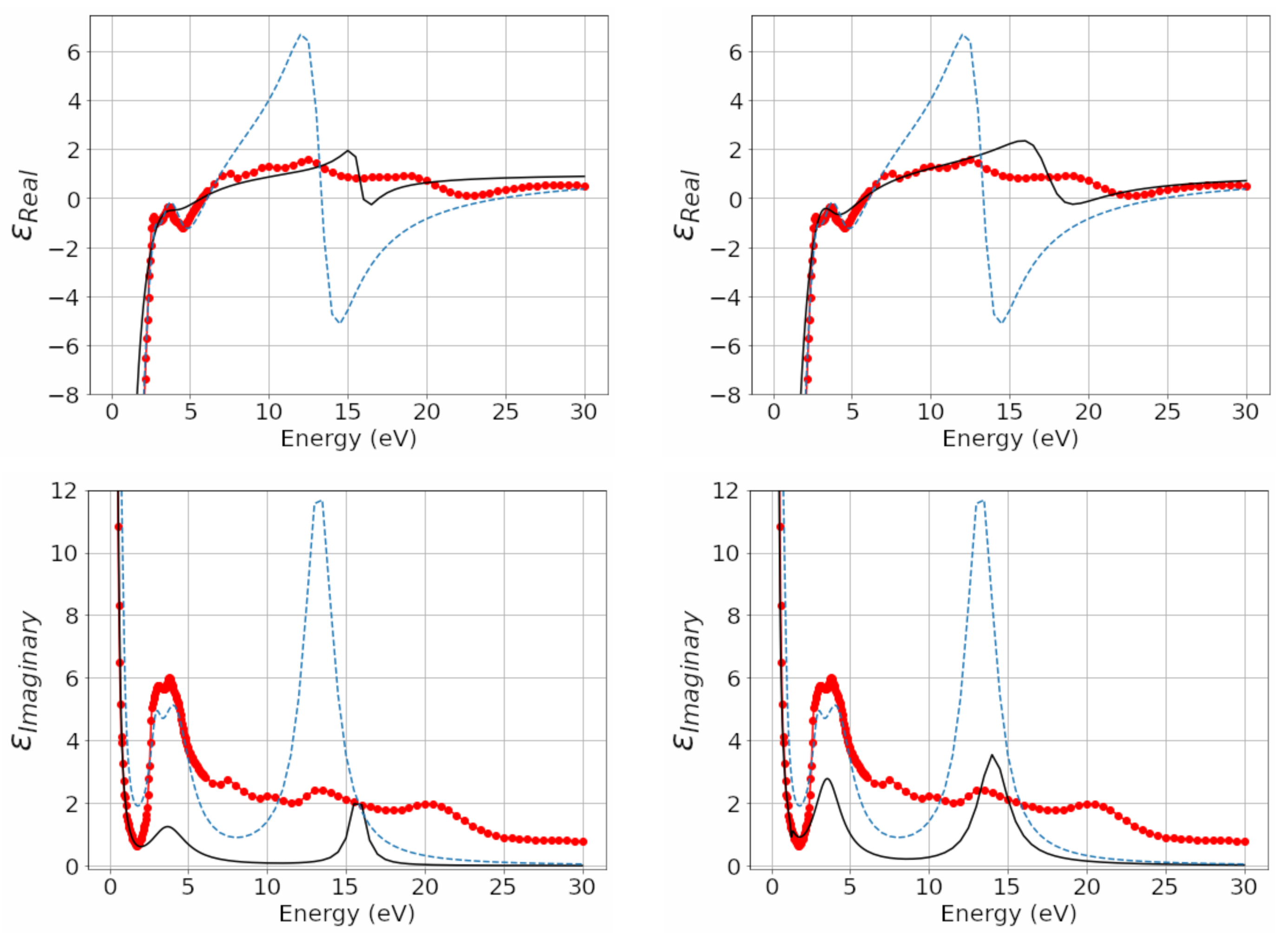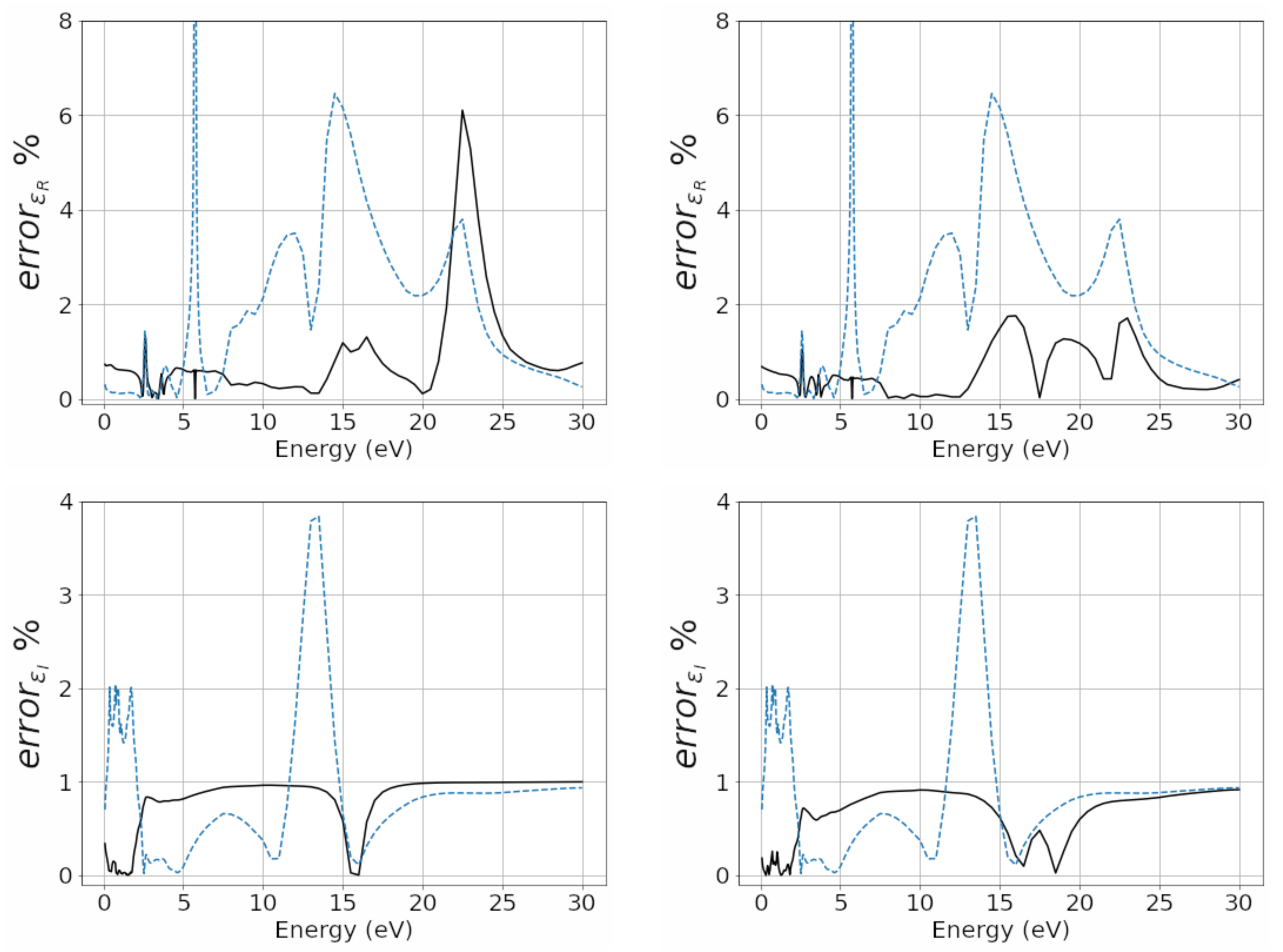In the left panels of Figure 4, we compare the the real and imaginary part trends of the complex permittivity, of the DL models by Rakic and the measurements obtained by Weaver; in the left panels of the same details are compared of the real and imaginary part trends of complex permittivity; the models of AL, Rakic and measurements obtained by Weaver. One can observe how the AL model is better than the DL model. In Figure 5, the relative complex permittivity errors in percent, compared to the corresponding experimental values, are reported in the left panels (upper panel the real part and lower panel the imaginary part) of the fractional models DL and Rakic; in the right panels of the same figure (upper panel the real part and lower panel the imaginary part) we report those of the models AL and Rakic. It can be observed that the trend of the relative percentage error of the DL fractional model is 1% lower for both the real and the imaginary part. The real part of the relative percentage error of the Rakic model is greater than 1% and around 6 eV is more than 50%.

With reference to the experimental silver data, applying the DE algorithm and using the objective function given by Equation (66), in

Table 6. Parameters of the DL fractional model for silver.

i	${\mathit{\alpha }}_{\mathit{i}}$	${\mathit{f}}_{\mathit{i}}$	${{\Gamma }}_{\mathit{i}}$	${\mathit{\omega }}_{\mathit{i}}$
0	0.995369	0.552911	0.020029	0.000000
1	1.607594	0.034764	1.802148	0.354432
2	2.016662	0.084785	0.249750	4.494656
3	1.083126	0.081158	0.046101	5.170580
4	1.200856	0.597546	0.098720	8.022841
5	1.077689	2.352133	6.752901	18.795728

and

Table 7. Parameters of the AL fractional model for silver.

i	${\mathit{\alpha }}_{\mathit{i}}$	${\mathit{f}}_{\mathit{i}}$	${{\Gamma }}_{\mathit{i}}$	${\mathit{\omega }}_{\mathit{i}}$	${{\Gamma }}_{\mathit{i},\mathit{s}}$
0	0.997125	0.564385	0.021641	0.000000	1.500000 $\times {10}^{-4}$
1	1.900155	0.076945	3.370088	0.467490	3.068187 $\times {10}^{-6}$
2	1.932523	0.113004	0.368817	1.942881	2.538806 $\times {10}^{-6}$
3	1.085868	0.084649	0.017738	5.215629	1.000000 $\times {10}^{-8}$
4	1.195181	0.561334	0.059148	8.017781	2.000000 $\times {10}^{-5}$
5	1.088296	2.422089	5.996217	19.064887	1.000000 $\times {10}^{-10}$

, the values of the parameters of the fractional model DL and AL are given. For model DL, you have a ${\omega }_{p_{{}_{DL}}}=11.99$ eV, whereas for model AL, you have a ${\omega }_{p_{{}_{AL}}}=11.94$ eV. It is observed how the fractional order of the relaxation equation describing the intraband component, represented by the Drude model, and the fractional orders of the relaxation equations related to the interband component, clearly deviate from the unit. In the left panels of Figure 6 of the real and imaginary part trends of the complex permittivity, the DL models, Rakic and the measurements obtained by Weaver are compared; in the left panels of the same figure we compare the real and imaginary part trends of complex permittivity, models of AL, Rakic and measurements obtained by Weaver. One can observe how the AL model is better than the DL model. In Figure 7, the relative complex permittivity errors in percent, compared to the corresponding experimental values, are reported in the left panels (upper panel the real part and lower panel the imaginary part) of the fractional models DL and Rakic; in the right panels of the same figure (upper panel the real part and lower panel the imaginary part), we report those of the models AL and Rakic. It can be observed that the trend of the relative percentage error of the DL fractional model is 1% lower for both the real and the imaginary part. The real part of the relative percentage error of the Rakic model is greater than 1% and around $7.5$ eV, 17 eV and $22.5$ eV is more than 50%.

Overall, the fractional models (CK-F) of Drude–Lorentz (DL) and Abraham–Lorentz (AL) are similar in energy values from tenths of electron volts to a few electron volt units, with a better fitting of the AL model than the DL model. For low energy values, the Rakic model condenses experimental data in a similar way to fractional models. For energy values of more than 5 eV, the Rakic model deviates from the experimental values both for the real part of permittivity, ${ϵ}_R$ and the imaginary part, ${ϵ}_I$. As for the fractional models, there is a better approximation of the AL model for the real part of permittivity than the DL model, whereas for the imaginary part, the fitting deviates from the experimental values without ever exceeding 2%; however, it should be noted that this deviation is justified by the assumption that the temperature at increasing frequency does not vary significantly to change the intra-band damping factor as foreseen in the previous section. The trend of the percentage error of the CK-F model is lower than the Rakic model.

9. Conclusions

Atoms are excited by high-frequency electromagnetic radiation. This results in a non-equilibrium scenario naturally fit to be investigated by the theoretical apparatus of de Groot and Mazur NET. An example in materials with relaxation is the well-known Raman effect (also known as inelastic scattering), which can be described by NET tools, which was one of our aims. Namely, in the first part of this work, we gave a theoretical explanation of the links between the behavior of electromagnetic materials with NET. In particular, we extend the Ciancio–Kluitenberg model [5] in the framework of fractional calculus. In physics, a material is endowed with ‘memory’ if the output variable (e.g., strain, polarization, etc.) does not only depend on the current physical status but also on previous times. This is mathematically modeled by means of a convolution integral—the Caputo fractional derivative—whose kernel can be read as a pulse response of the system; thus, the fractional exponent can be considered as a measure of the memory of the material. For dielectrics, this index is in the interval (0,1). In metals, the Caputo fractional derivative represents a larger sensitivity to large frequencies (or, equivalently, energies). In particular, we think that the intra- and inter-band transition at very high frequencies determine the above-mentioned memory effect. Our model represents these complex phenomena via a phenomenological model where multiple components (each with a distinct memory index) are taken into the account.

After building the above-mentioned theoretical model, we also validated it, and showed that our approach can be considered as an improvement of previous studies.

Namely, under the hypothesis of quasi-stationarity and superimposability of intra-band and inter-band interaction, the proposed CK-F model is in good agreement with experimental data on a frequency spectrum from infrared to ionizing radiation such as X-rays, i.e., not only in the frequency range typical of mechanical vibrations and for electrically insulating materials but also for plasmonic materials at electronic frequencies. The system consists of a number of subsystems each characterized by a fractional differential equation of relaxation whose overlap is the result of the interaction due to inter-band and intra-band transitions of electrons.

References

1. De Groot, S.R.; Mazur, P. Non-Equilibrium Thermodynamics; Dover Publications, Inc.: New York, NY, USA, 1984; pp. 1–528. [Google Scholar]
2. Gyarmati, I. Non-Equilibrium Thermodynamics: Field Theory and Variational Principles; Springer: Berlin/Heidelberg, Germany, 1970; pp. 1–184. [Google Scholar]
3. Ciancio, V. Non Equilibrium Thermodynamics with internal variables in Kluitenberg’s theory. AAPP 2008, 86, 1–14. [Google Scholar]
4. Kluitenberg, G.A. On vectorial internal variables and dielectric and magnetic relaxation phenomena. Phys. A Stat. Mech. 1981, 109, 91–122. [Google Scholar] [CrossRef]
5. Ciancio, V.; Kluitenberg, G.A. On electromagnetic waves in isotropic media with dielectric relaxation. Acta Phys. Hung. 1989, 66, 251–276. [Google Scholar] [CrossRef]
6. Ciancio, V.; Ciancio, A.; Farsaci, F. Phenomenological and state coefficients for poly-isobutylene in Kluitenberg-Ciancio theory. Commun. SIMAI Congr. 2006, 1, 1–3. [Google Scholar]
7. Ciancio, A.; Ciancio, V.; Farsaci, F. Rheological Coefficients for Media with Mechanical Relaxation Phenomena. Commun. SIMAI Congr. 2007, 2, 1–6. [Google Scholar]
8. Ciancio, V.; Farsaci, F.; Rogolino, P. On the Extension of Debye’s Model for Media with dielectric relaxation. Int. J. Eng. Interdiscip. Math. 2009, 1, 57–63. [Google Scholar]
9. Farsaci, F.; Rogolino, P. An alternative dielectric model for low and high frequencies: A non-equilibrium thermodynamic approach. J. Non-Equil. Thermodyn. 2012, 37, 27–41. [Google Scholar] [CrossRef]
10. Ciancio, A.; Flora, B.F.F. A Fractional Complex Permittivity Model of Media with Dielectric Relaxation. Fractal Fract. 2017, 1, 4. [Google Scholar] [CrossRef] [Green Version]
11. Alabastri, A.; Tuccio, S.; Giugni, A.; Toma, A.; Liberale, C.; Das, G.; De Angelis, F.; Di Fabrizio, E.; Zaccaria, R. Proietti Molding of plasmonic resonances in metallic nanostructures: Dependence of the non-linear electric permittivity on system size and temperature. Materials 2013, 6, 4879–4910. [Google Scholar] [CrossRef] [Green Version]
12. Karpiński, K.; Zielińska-Raczyńska, S.; Ziemkiewicz, D. Fractional Derivative Modification of Drude Model. Sensors 2021, 21, 4974. [Google Scholar] [CrossRef]
13. Rioux, D.; Vallières, S.; Besner, S.; Muñoz, P.; Mazur, E.; Meunier, M. An analytic model for the dielectric function of Au, Ag, and their alloys. Adv. Opt. Mater. 2014, 2, 176–182. [Google Scholar] [CrossRef]
14. Landi, G.T.; Paternostro, M. Irreversible entropy production: From classical to quantum. Rev. Mod. Phys. 2021, 93, 035008. [Google Scholar] [CrossRef]
15. Purcell, E.M. Electricity and Magnetism Vol.2. Berkeley Physics Course; Mcgraw-Hill: New York, NY, USA, 1965; pp. 1–459. [Google Scholar]
16. Griffiths, D.J. Introduction to the Electrodynamics; Pearson Education: London, UK, 2013; pp. 1–623. [Google Scholar]
17. Nickelson, L. Electromagnetic Theory and Plasmonics for Engineers; Springer: Singapore, 2019; pp. 1–749. [Google Scholar]
18. Tarasov, V.E. No nonlocality. No fractional derivative. Commun. Nonlinear Sci. Numer. Simul. 2018, 62, 157–163. [Google Scholar] [CrossRef] [Green Version]
19. Caputo, M. Linear Models of Dissipation whose Q is almost Frequency Independent—II. Geophys. J. Int. 1967, 13, 529–539. [Google Scholar] [CrossRef]
20. Tarasov, V.E.; Tarasova, S.S. Fractional Derivatives and Integrals: What Are They Needed For? Mathematics 2020, 8, 164. [Google Scholar] [CrossRef] [Green Version]
21. Bohren, C.F.; Huffman, D.R. Absorption and Scattering of Light by Small Particles; WILEY-VCH: Weinheim, Germany, 1998; pp. 1–530. [Google Scholar]
22. Li, M.F.; Ren, J.R.; Zhu, T. Fractional vector calculus and fractional special function. arXiv 2010, arXiv:1001.2889. [Google Scholar]
23. Kluitenberg, G.A. On dielectric and magnetic relaxation phenomena and non-equilibrium thermodynamics. Physica 1973, 68, 75–92. [Google Scholar] [CrossRef]
24. Kluitenberg, G.A. On dielectric and magnetic relaxation phenomena and vectorial internal degrees of freedom in thermodynamics. Phys. A Stat. Mech. 1977, 87, 302–330. [Google Scholar] [CrossRef]
25. Restuccia, L.; Kluitenberg, G.A. On generalizations of the Debye equation for dielectric relaxation. Phys. A Stat. Mech. 1988, 154, 157–182. [Google Scholar] [CrossRef]
26. Kats, M.; Yu, N.; Genevet, P.; Gaburro, Z.; Capasso, F. Effect of radiation damping on the spectral response of plasmonic components. Opt. Express 2011, 19, 21748–21753. [Google Scholar] [CrossRef] [Green Version]
27. Ehrenreich, H.; Philipp, H.R.; Segall, B. Optical properties of aluminum. Phys. Rev. 1963, 132, 1918–1928. [Google Scholar] [CrossRef]
28. Ehrenreich, H.; Philipp, H.R. Optical properties of Ag and Cu. Phys. Rev. 1962, 128, 1622–1629. [Google Scholar] [CrossRef]
29. Rakić, A.D.; Djurišić, A.B.; Elazar, J.M.; Majewski, M.L. Optical properties of metallic films for vertical-cavity optoelectronic devices. Appl. Opt. 1998, 37, 5271–5283. [Google Scholar] [CrossRef]
30. John, H. Weaver Department of Materials Science and Engineering. Available online: http://jhweaver.matse.illinois.edu/optical-prop/optical-constantsCuAgAu.pdf (accessed on 21 April 2022).
31. SciPy v1.8.0 Manual. Available online: https://docs.scipy.org/doc/scipy/reference/generated/scipy.optimize.differential_evolution.html (accessed on 21 April 2022).
32. Storn, R.M.; Price, K. Differential evolution—A simple and efficient heuristic for global optimization over continuous spaces. J. Glob. Optim. 1997, 4, 341–359. [Google Scholar] [CrossRef]
33. Price, K.; Storn, R.M.; Lampinen, J.A. Differential Evolution: A Practical Approach to Global Optimization; Springer: Berlin/Heidelberg, Germany, 2005; pp. 1–539. [Google Scholar]
34. Johansson, R. Numerical Python: A Practical Techniques Approach for Industry; Apress: Berkeley, CA, USA, 2015; pp. 1–487. [Google Scholar]
35. Djurisic, A.B.; Rakic, A.D.; Elazar, J.M. Modeling the optical constants of solids using acceptance-probability-controlled simulated annealing with an adaptive move generation procedure. Phys. Rev. E 1997, 55, 4797–4803. [Google Scholar] [CrossRef] [Green Version]
36. Liouville, J. Mémoire sur le calcul des différentielles à indices quelconques. J. de l’Ecole Pol. 1832, 13, 71–162. [Google Scholar]
37. Letnikov, A.V. Theory of differentiation of an arbitrary order. Mat. Sb. 1868, 3, 1–68. [Google Scholar]
38. Sonin, N.Y. On differentiation with arbitrary index. Moscow Matem. Sbornik 1869, 6, 1–38. [Google Scholar]
39. Weyl, H. Bemerkungen zum begriff des differentialquotienten gebrochener ordnung. Vierteljschr. Naturforsch. Gesellsch 1917, 62, 296–302. [Google Scholar]
40. Samko, S.; Kilbas, A.A.; Marichev, O. Fractional Integrals and Derivatives; Gordon and Breach Science Publishers: Amsterdam, The Netherlands, 1993; pp. 1–1016. [Google Scholar]
41. Erdélyi, A. Asymptotic Evaluation of Integrals Involving a Fractional Derivative. SIAM J. Math. Anal. 1974, 5, 159–171. [Google Scholar]
42. Kober, H. On fractional integrals and derivates. Q. J. Math. 1940, 11, 193–211. [Google Scholar] [CrossRef]
43. Caputo, M.; Fabrizio, M. A new definition of fractional derivative without singular kernel. Prog. Fract. Differ. Appl. 2015, 1, 73–85. [Google Scholar]
44. Ciancio, V.; Flora, B.F.F. Technical Note on a New Definition of Fractional Derivative. Progr. Fract. Differ. Appl. 2017, 3, 233–235. [Google Scholar] [CrossRef]
45. Khalil, R.; Al Horani, M.; Yousef, A.; Sababheh, M. A new definition of fractional derivative. J. Comput. Appl. Math. 2014, 264, 65–70. [Google Scholar] [CrossRef]
46. Anderson, D.R.; Ulness, D.J. Properties of the Katugampola fractional derivative with potential application in quantum mechanics. J. Math. Phys. 2015, 56, 063502. [Google Scholar] [CrossRef] [Green Version]
47. Sousa, J.V.C.; Oliveira, E.C. A new truncated M-fractional derivative type unifying some fractional derivative types with classical properties. Int. J. Anal. Appl. 2018, 16, 83–96. [Google Scholar]
Figure 1. Reference system in spherical coordinates: distance OA.
Fractalfract 06 00390 g001
Figure 2. Permittivity of the copper. Panels left: fractional model DL. Panels right: fractional model AL. Black line: this work. Line with blue dashed: Rakic. Red dotted line: measures of J.H.Weaver.
Fractalfract 06 00390 g002
Figure 3. Copper—relative percentage error: Panels left: fractional model DL. Panels right: fractional model AL. Black line: this work. Line with blue dashed: Rakic.
Fractalfract 06 00390 g003
Figure 4. Permittivity of the gold. Panels left: fractional model DL. Panels right: fractional model AL. Black line: this work. Line with blue dashed: Rakic. Red dotted line: measures of J.H.Weaver.
Fractalfract 06 00390 g004
Figure 5. Gold—relative percentage error: Panels left: fractional model DL. Panels right: fractional model AL. Black line: this work. Line with blue dashed: Rakic.
Fractalfract 06 00390 g005
Figure 6. Permittivity of the silver. Panels left: fractional model DL. Panels right: fractional model AL. Black line: this work. Line with blue dashed: Rakic. Red dotted line: measures of J.H.Weaver.
Fractalfract 06 00390 g006
Figure 7. Silver—relative percentage error: Panels left: fractional model DL. Panels right: fractional model AL. Black line: this work. Line with blue dashed: Rakic.
Fractalfract 06 00390 g007