Article

Sign Retention in Classical MF-DFA

School of Mathematics and Statistics, Nanjing University of Information Science and Technology, Nanjing 210044, China
*
Author to whom correspondence should be addressed.
Fractal Fract. 2022, 6(7), 365; https://doi.org/10.3390/fractalfract6070365
Submission received: 25 May 2022 / Revised: 23 June 2022 / Accepted: 25 June 2022 / Published: 30 June 2022

Abstract

:
In this paper, we propose a one-dimensional (1D) multifractal sign retention detrending fluctuation analysis algorithm (MF-S-DFA). The proposed method is based on conventional multifractal detrending fluctuation analysis (MF-DFA). As negative values may exist in the calculation in the original MF-DFA model, sign retention is considered to improve performance. We evaluate the two methods based on time series constructed by p-model multiplication cascades. The results indicate that the generalized Hurst exponent H ( q ) , the scale exponent τ ( q ) and the singular spectrum f ( α ) estimated by MF-S-DFA behave almost consistently with the theoretical values. Moreover, we also employ distance functions such as D H and D τ . The results prove that MF-S-DFA achieves more accurate estimation. In addition, we present various numerical experiments by transforming parameters such as n m a x , q and p. The results imply that MF-S-DFA obtains more excellent performance than that of conventional MF-DFA in all cases. Finally, we also verify the high feasibility of MF-S-DFA in ECG signal classification. Through classification of normal and abnormal ECG signals, we further corroborate that MF-S-DFA is more effective than conventional MF-DFA.

1. Introduction

As a branch of nonlinear mathematics, multifractal methods have been widely used in various research fields [1,2,3,4]. For time series, it may be difficult to explain the scale change of probability distribution using simple fractals because simple fractals can only capture a certain aspect of time series changes without considering local features. However, multifractals can more effectively dig out, reveal and predict the inner law of time series.
Since Kantelhardt et al. [5] considered q-order fluctuations on the basis of DFA [6], multifractal detrending fluctuation analysis (MF-DFA) quickly became the dominant method for financial and other time series. Afterwards, Podobnik and Stanley introduced detrended cross-correlation analysis of non-stationary time series [7], and Zhou et al. [8] extended it to analyze multifractal time series. The advantage of MF-DFA is in discovering long-range correlation of non-stationary time series and avoiding misjudgment of correlation. In the feature analysis of one-dimensional time series, such as financial [9,10,11], traffic flow [12,13,14], air pollution indexes [15,16], DNA sequencing [17,18], ECG signal sequencing [19,20], etc., MF-DFA can reveal the multifractal characteristics and long-range correlation of these time series, as well as the cross-correlation multifractal characteristics and the existence of interconnection between two sets of sequences.
In recent years, high-dimensional fractal and multifractal feature testing based on time series and images has made great progress, promoting the development of various technologies. The performance of conventional MF-DFA is gradually increasing in real life and has achieved remarkable results [21,22,23,24]. Lavicka et al. [25] analyzed the electric power load time series of 35 independent countries and improved the basic MF-DFA with unified shuffling and substitution of the dataset to prove the robustness of the results to nonlinear effects. Sosa-Herrera et al. [26] proposed a method based on kernel density that provides an error index for estimation of the multi-fractal spectrum obtained by MF-DFA, and gave the probability of error within a certain range at each moment in the spectrum. Comparison between this method and the traditional methods applied to deterministic and random multiplication processes proved the robustness of false estimation of generalized fractals in MF-DFA.
Inspired by MF-DFA, we consider replacing the residual sign in conventional MF-DFA with the mean square error sign. When calculating the mean square error in the fourth step of conventional MF-DFA, the result is positive. However, the improved model incorporates the positive and negative characteristics of the traditional residual sequence into the calculation of the mean square error. Therefore, the algorithm proposed in this paper is called MF-S-DFA. Multiplication cascading is used to generate the multiplication cascade time series of the p-model proposed to test the performance of the proposed MF-S-DFA method [27]. The generalized Hurst exponent H ( q ) , the scale exponent τ ( q ) and the singular spectrum f ( α ) of MF-S-DFA are compared with the theoretical values. In addition, we calculate and compare the two methods for the standard deviation of H e r r and τ e r r , and calculate D H and D τ by changing parameters such as n m a x , q and p to further prove that the proposed method is effective. Finally, using ECG signals, we verify whether MF-S-DFA is more effective than conventional MF-DFA for practical problems.
The rest of this paper is organized as follows. We provide the description of MF-S-DFA in Section 2. We present MF-S-DFA numerical experiments in Section 3. Then, we present application of MF-S-DFA in Section 4. Conclusions are given in Section 5.

2. Methodology

All the computations are processed using MATLAB R2018b on a computer with an Intel(R) Core(TM) i5-6200 CPU @ 2.30 GHz.

2.1. Multiplicative Cascades Series

In this paper, to estimate the performance of the proposed MF-S-DFA method, we use the p-model algorithm to generate the multiplicative cascades series. Here is a specific description of the p-model:
X i = p n ( i 1 ) ( 1 p ) n m a x n ( i 1 ) ,
where 0.5 < p < 1 , i = 1 , 2 , , N . N = 2 n m a x is the length of the generated time series, where n m a x is a power of 2. i in n ( i ) denotes the binary representation, and n ( i ) represents the number of 1 in the binary representation number.
The initial multiplicative cascading time series has parameters p = 0.75 and n m a x = 10, as shown in Figure 1.
We calculate the theoretical value of the scale exponent τ ( q ) by
τ ( q ) = ln [ p q + ( 1 p ) q ] ln 2 .
Moreover, the theoretical value of the generalized Hurst exponent H ( q ) can be determined by
H ( q ) = τ ( q ) + 1 q , i f q = 0 , ln [ p ( 1 p ) ] 2 ln 2 , o t h e r w i s e .
Then, the theoretical values of the singularity exponent α and the singularity spectrum f ( α ) can be obtained as
α ( q ) = p q l n p + ( 1 p ) q l n ( 1 p ) [ p q + ( 1 p ) q ] l n 2 ,
f ( α ) = q p q l n p + q ( 1 p ) q l n ( 1 p ) [ p q + ( 1 p ) q ] l n 2 + l n [ p q + ( 1 p ) q ] l n 2 .
For the experimental tests, we fix parameters such as window size s [ 35 , 105 ] with an increment of 11, the order q [ 20 , 20 ] with a total number of 21; p = 0.75 , and n m a x = 10 .

2.2. MF-S-DFA

Among the steps of the traditional MF-DFA algorithm, one of the steps is:
ϵ i = X i X ^ i , i = 1 , 2 , , M .
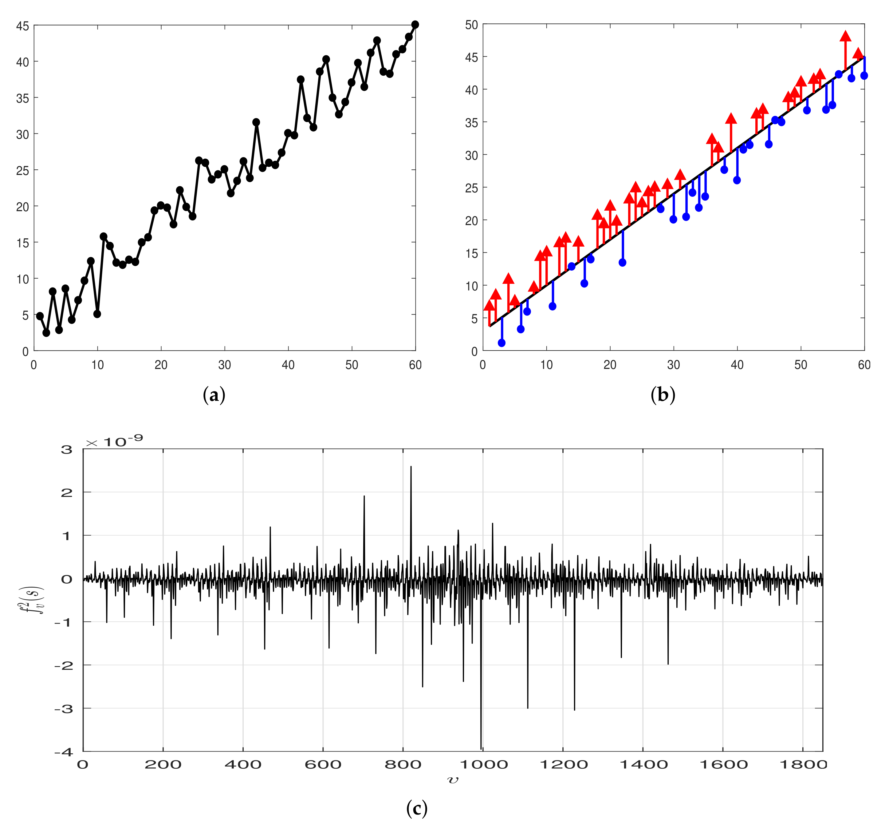
When i approaches a certain value, a negative value may appear, resulting in complex valued quantities. For instance, we want to fit the time series as shown in Figure 2a. The black line in Figure 2b is first-order polynomial fitting X ^ i , the point above the black line is represented by a red upper triangle, and the point below the black line is represented by a blue circle. It is obvious that Equation (6) has a high probability of a negative value. In addition, the negative values in Equation (7) are eliminated, but they actually exist.
f v ( s ) = 1 s t = 1 s [ x v x ^ v ] 2 .
Figure 2c shows our intention for sign retention, f v 2 ( s ) obtained by MF-S-DFA, and we can clearly see that there are negative values.
In order to solve this problem, we propose MF-S-DFA; the difference being that sign retention is considered in the original algorithm structure. Here is a brief introduction of the proposed model. We construct a multiplication cascade time series based on the p-model, then calculate the cumulative sequence as follows
x i = k = 1 i ( X k X ¯ ) , i = 1 , 2 , , M ,
where X ¯ = i = 1 M X i / M .
The time series is partitioned into M s = [ M / s ] non-overlapping windows of size s, and the v th window is referred to as [ l v + 1 , l v + s ] , where l v = ( v 1 ) s . Then, the time series of the v th window is x v = [ x ( l v + 1 ) , , x ( l v + s ) ] . Subsequently, we calculate the square mean of the 2 M s elimination trend sub-interval sequence,
f v ( s ) = 1 s t = 1 s s i g n [ x v x ^ v ] [ x v x ^ v ] 2 ,
where x ^ v is the local trend function on each sub-area v calculated by the least square method.
The last step is to compute the q-th order fluctuation function,
F q ( s ) = 1 2 M s v = 1 2 M s s i g n [ f v ( s ) ] | f v ( s ) | q 2 1 q , i f q 0 , exp 1 4 M s v = 1 2 M s ln | f v ( s ) | , i f q = 0 .
For both MF-DFA and MF-S-DFA, the scaling relation follows
F q ( s ) s H ( q ) ,
where H ( q ) is the required generalized Hurst exponent.
The singularity strength and probability distribution of multifractal systems is usually described by the scale exponent τ ( q ) , defined by
τ ( q ) = q h ( q ) 1 .
According to Legendre transformation [28], the singularity strength α and the fractal dimension f ( α ) can be expressed as
α = τ ( q ) = h ( q ) + q h ( q ) ,
f ( α ) = q [ α h ( q ) ] + 1 .

3. Emperiment Results

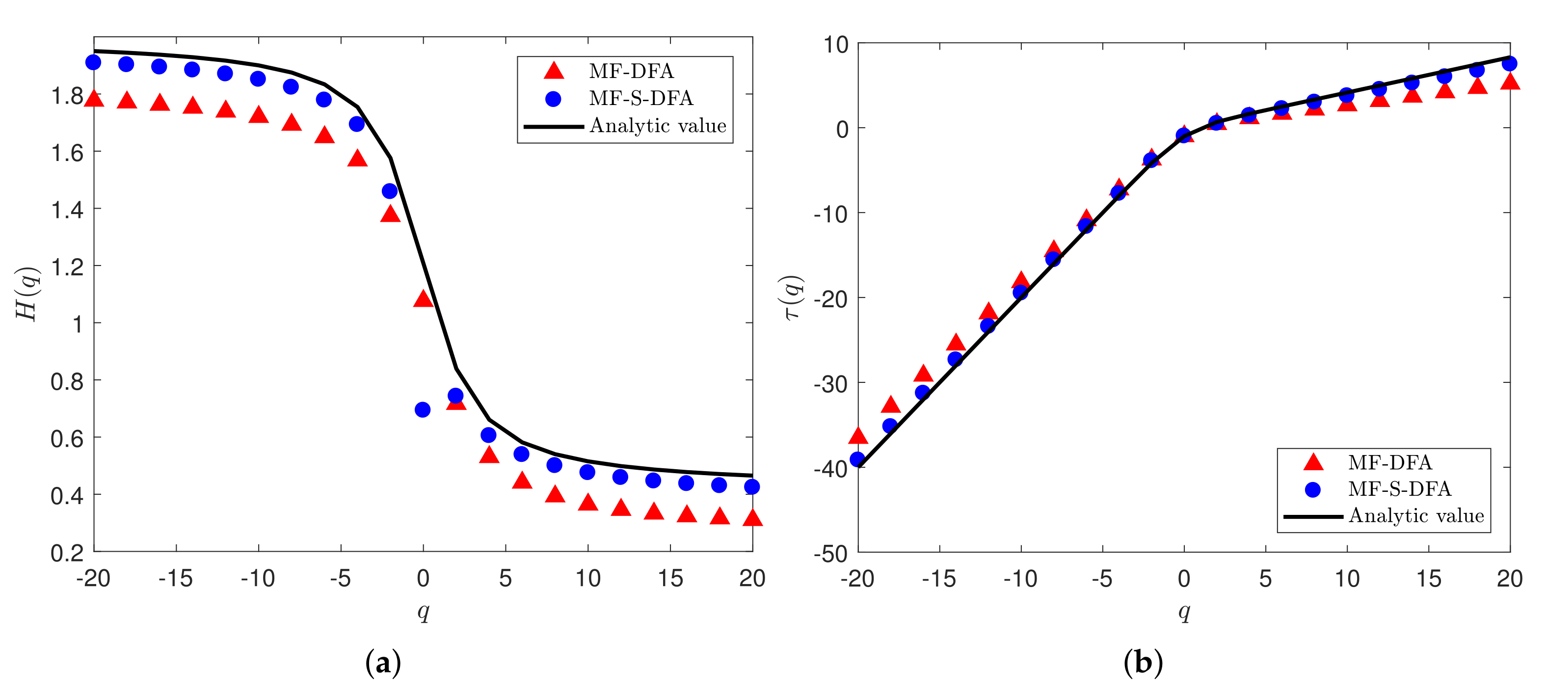
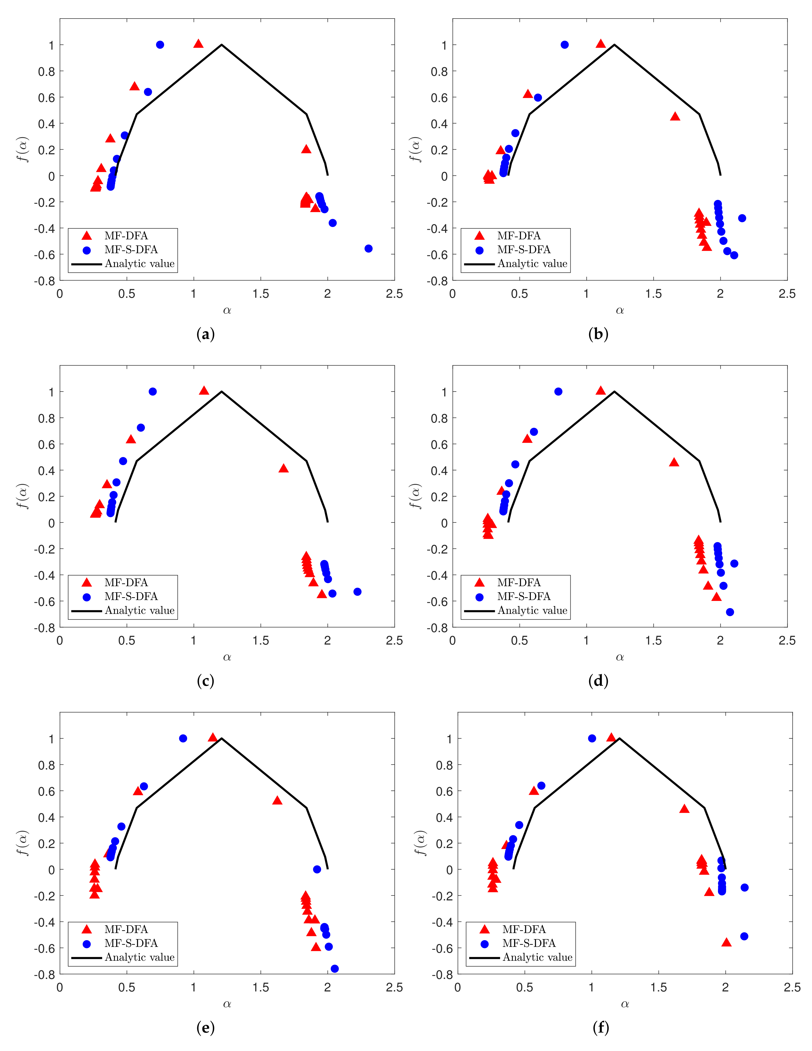
In this section, we perform various numerical experiments to show the robustness of the proposed MF-S-DFA. We calculate the values of the multifractal feature according to q, which varies from 20 to 20 with intervals of 21. The numerical and analytical values of the generalized Hurst exponent H ( q ) , the scale exponent τ ( q ) and the singular spectrum f ( α ) of the two methods are calculated. In Figure 3a,b, the black line represents the theoretical value, the red triangle represents the MF-DFA numerical solution, and the blue solid dot represents the MF-S-DFA numerical solution. It can be seen that their distribution trends are consistent and close to the theoretical values. However, MF-S-DFA, represented by the blue solid point, is closer to the theoretical values. Furthermore, we compare the singular spectrum f ( α ) of MF-DFA and MF-S-DFA with the theoretical values by changing the value of the parameter n m a x . We also see from Figure 4 that their distribution trends are consistent, and the numerical values of MF-S-DFA are closer to the theoretical values. It is undeniable that the proposed MF-S-DFA is a great improvement over conventional MF-DFA, with the multifractal characteristic curve closer to the theoretical value.
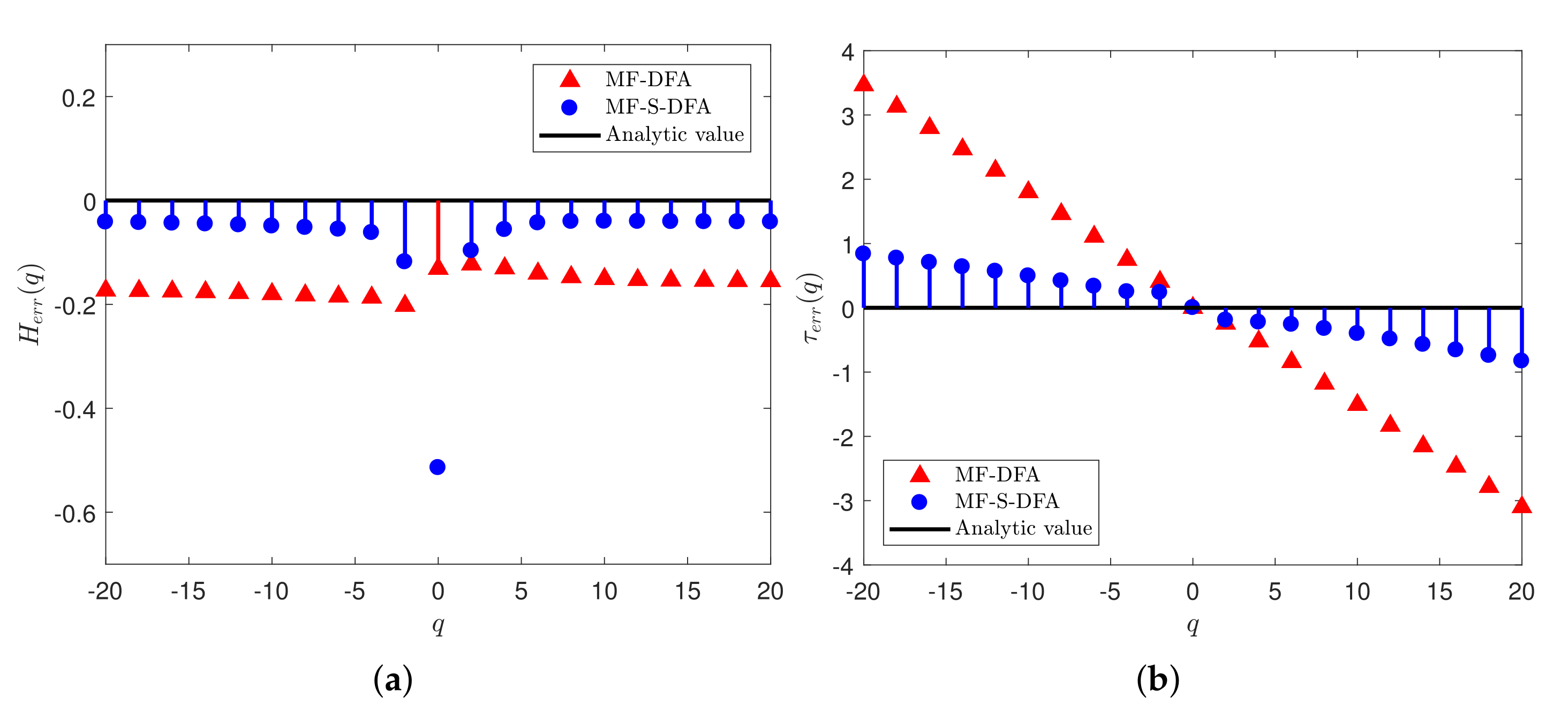
In order to further quantify the difference between the two methods and the theoretical value, we use relative errors H e r r ( q ) = H ( q ) H a n ( q ) and τ e r r ( q ) = τ ( q ) τ a n ( q ) . Among them, H a n and τ a n are analytical values. For further visualization, we depict the metrics in Figure 5a,b. The black straight line represents the theoretical error value, and the red and blue marks represent MF-DFA and MF-S-DFA, respectively. We connect the points closer to the theoretical value with the theoretical straight line by line segments, with more points connected to the analytical value indicating the corresponding method is better. From both Figure 5a,b, we observe that the proposed MF-S-DFA method has more excellent performance.
Furthermore, we develop the distance function D H = ( H e r r ( q ) ) 2 n to calculate the overall distance between the generalized Hurst exponent numerical solutions and the theoretical solutions. Similarly, D τ = ( τ e r r ( q ) ) 2 n is adopted for measuring the numerical solution of the scale exponents and the corresponding theoretical values. That is, the smaller the distance between D H and D τ , the higher the effectiveness and accuracy of the corresponding method. From Table 1, we note that for both D H and D τ , the values of MF-S-DFA are less than those of MF-DFA, implying the MF-DFA model with sign retention is more suitable for the real multifractal characteristics of time series.
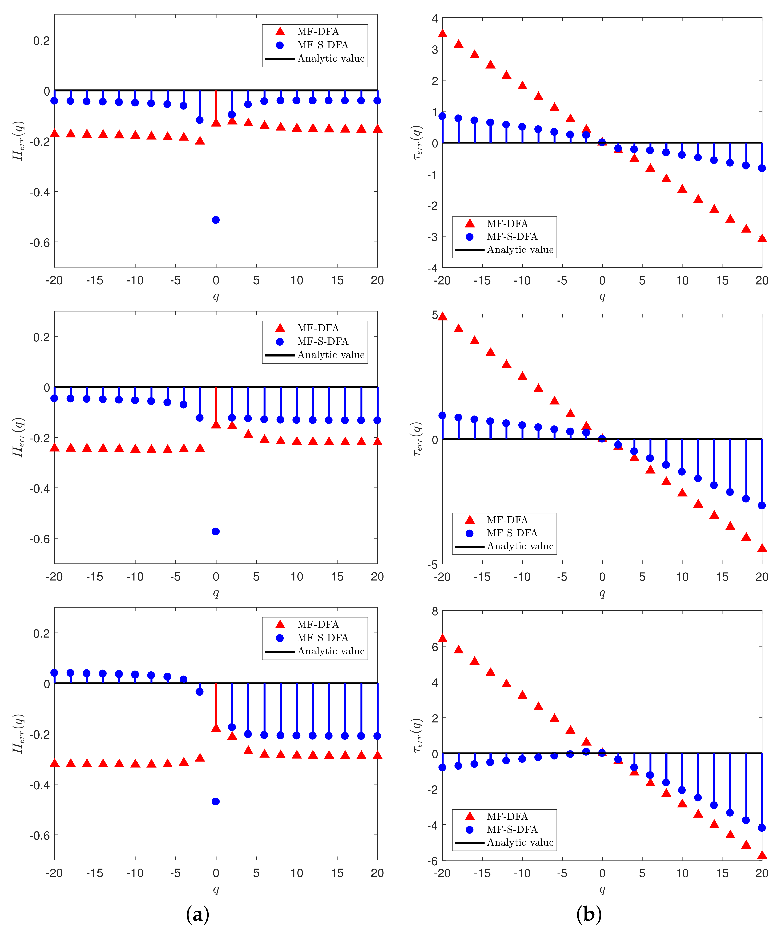
In order to quantitatively estimate the performance of the proposed MF-S-DFA method, in the following tests, we evaluate the efficiency of the proposed MF-S-DFA by changing the parameters. We adjust the parameters n m a x , p and q to compare H e r r ( q ) and τ e r r ( q ) of the two multifractal methods.

3.1. Multifractal Analysis with Different n m a x

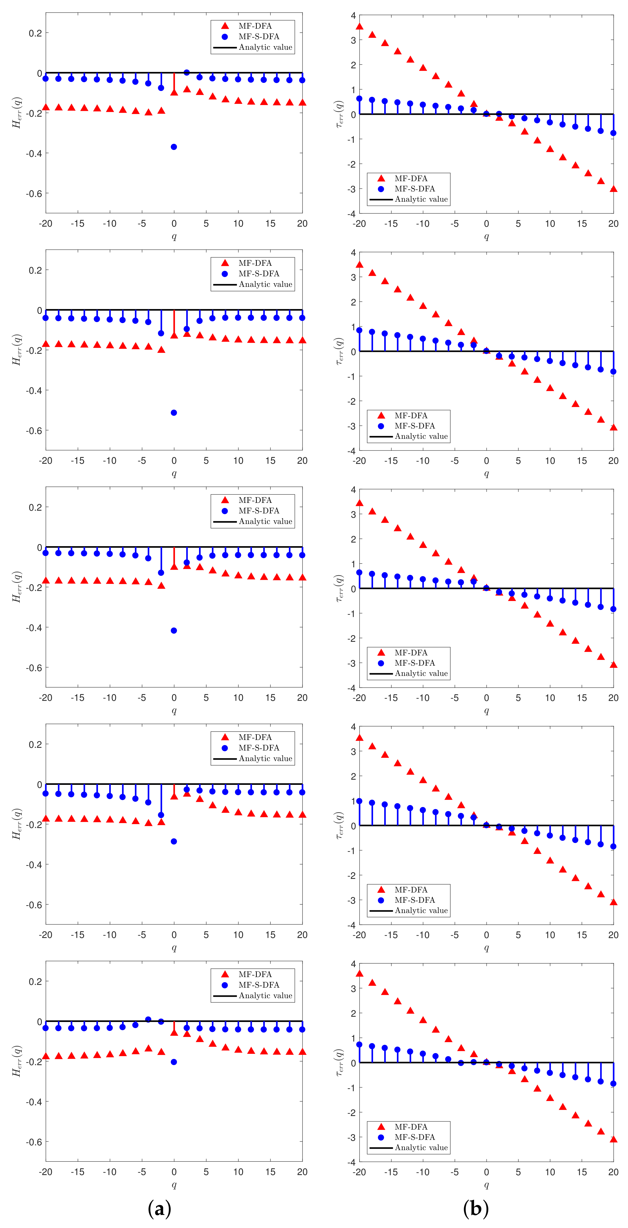
In this section, the parameter n m a x is set to 8, 9, 10, 11, 12 or 13 to calculate multifractal features. The H e r r ( q ) and τ e r r ( q ) with these parameters for the two methods are calculated, and the values are depicted in Figure 6. We observe that changing n m a x does not affect our previous conclusions. For both H ( q ) and τ ( q ) , the blue dots are closer to the black lines, which means that compared with MF-DFA, the numerical solutions of generalized Hurst exponent and the scale exponent of MF-S-DFA are more consistent with the theoretical solutions and can more effectively describe the multifractal characteristics of time series. Figure 6 represents the distribution of n m a x = 8 , 9 , 10 , 11 , 12 and 13, respectively, from top to bottom.
Similarly, as shown in Table 1 (smaller values are shown in bold), we observe that for each n m a x , the D H and D τ of MF-S-DFA are smaller than those of MF-DFA. The results show that MF-S-DFA is superior to traditional MF-DFA.

3.2. Multifractal Analysis with Different Domains of q

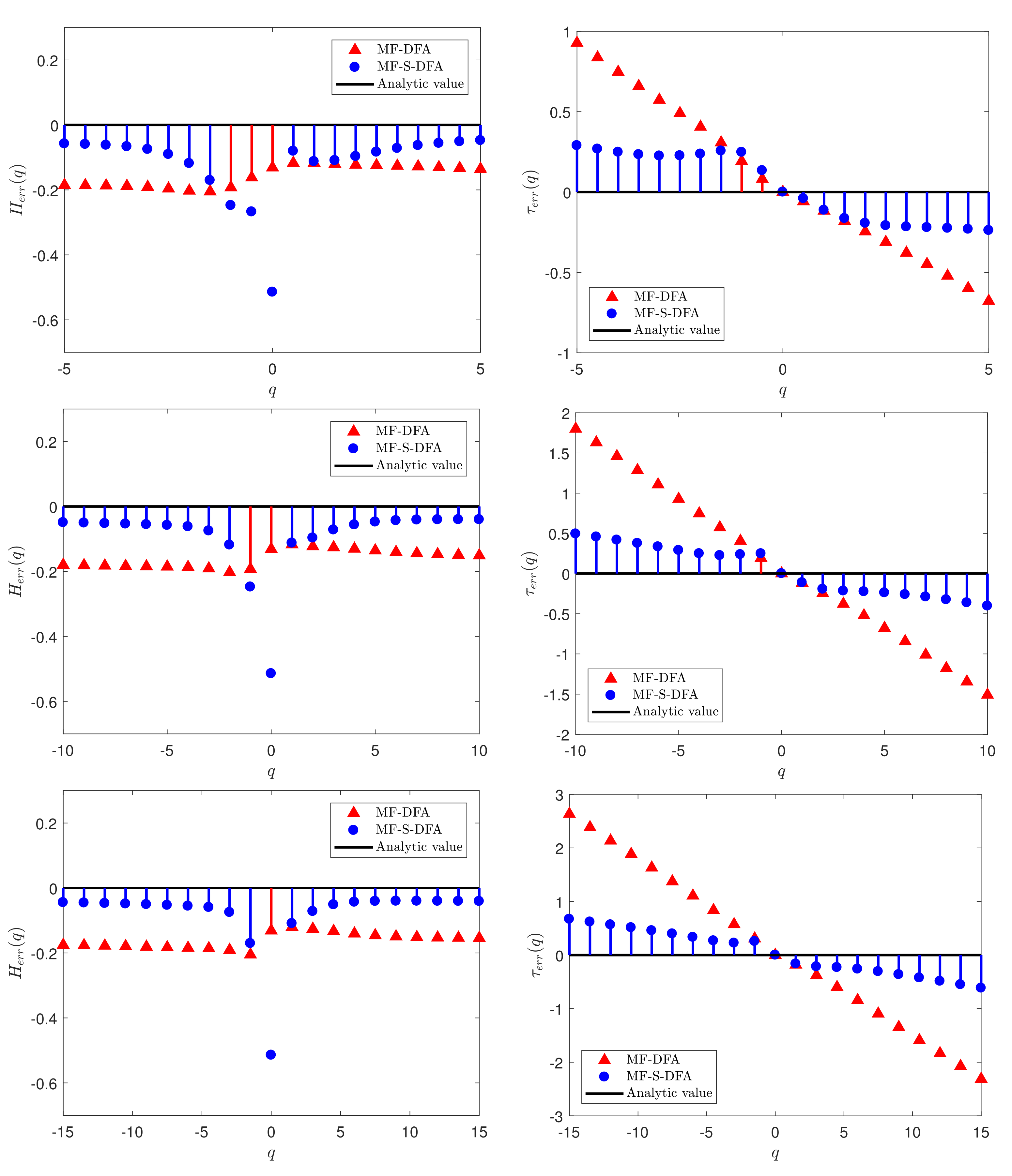
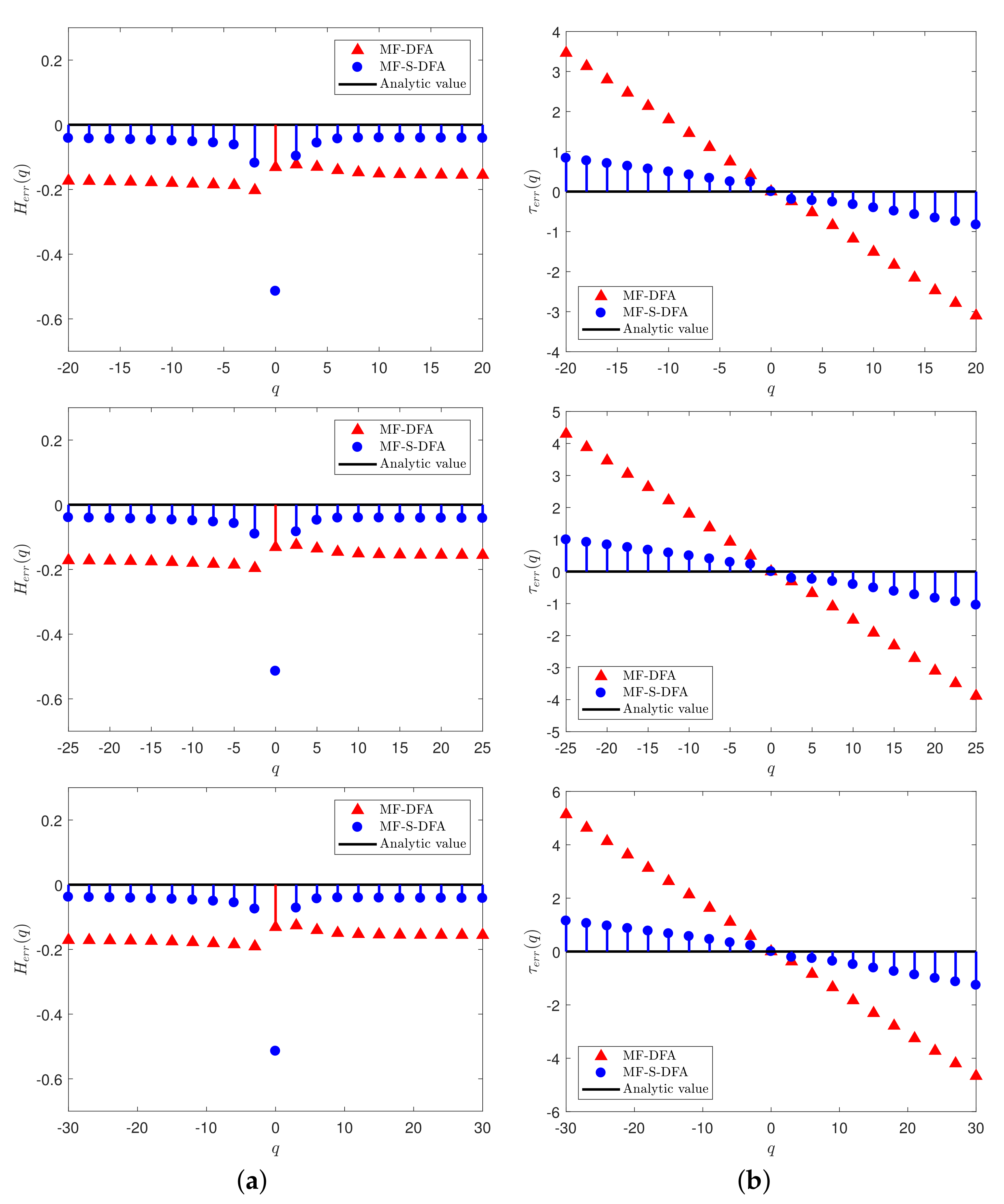
In this section, we focus on another parameter, q. A group of domains of q such as [ 5 , 5 ] , [ 10 , 10 ] , [ 15 , 15 ] , [ 20 , 20 ] , [ 25 , 25 ] and [ 30 , 30 ] are selected to calculate multifractal features. We also assess the two methods by comparing the H e r r ( q ) and τ e r r ( q ) . In Figure 7, the results indicate that our proposed method achieves better performance. In addition, we adopt the distance function D H and D τ to quantitatively describe the differences between MF-S-DFA and MF-DFA. We compute all the values of MF-DFA and MF-S-DFA under different domains of q in Table 2. For comparison of the two methods, a smaller value represent more excellent performance, and the smaller values are shown in bold in Table 2. Table 2 exhibits that the proposed MF-S-DFA performs significantly better than traditional MF-DFA.

3.3. Multifractal Analysis with Different p

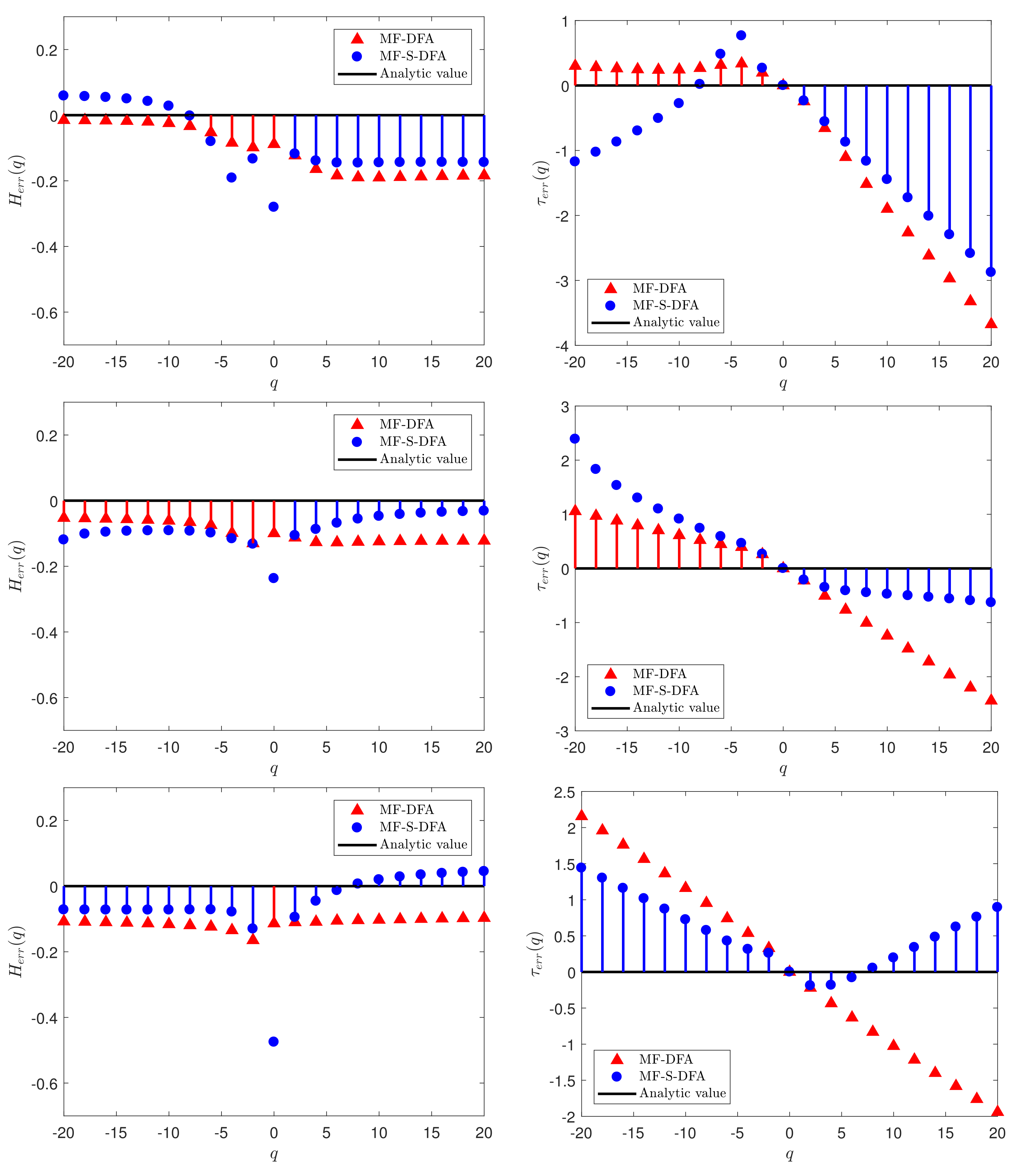
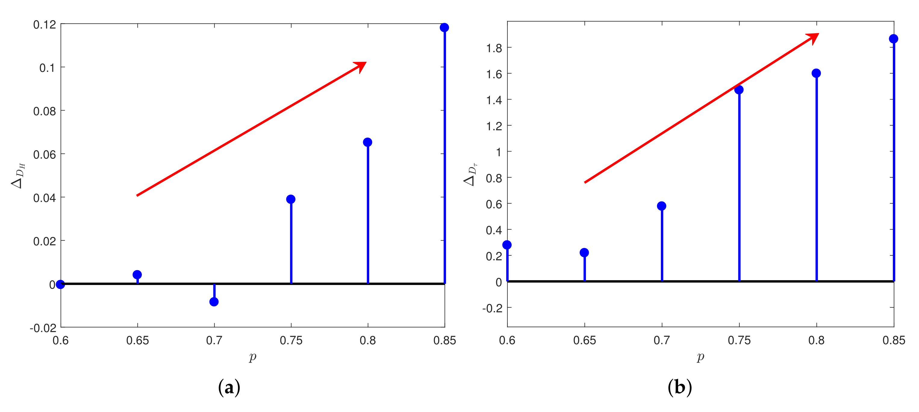
Now we investigate the parameter p, which is a significant parameter used to generate multiplicative cascade time series in p models. We choose the value of p with a set of varying values such as 0.60 , 0.65 , 0.70 , 0.75 , 0.80 and 0.85 to calculate the multifractal properties. As shown in Figure 8, for the relative errors H e r r ( q ) and τ e r r ( q ) under each p, most of the blue solid points representing MF-S-DFA are closer to the theoretical values than the red upper triangles representing MF-DFA. The same conclusion can be obtained from Table 3, and it can be seen that different from the previous two groups of experiments, when the value of p is slightly smaller, the advantages of MF-S-DFA are not obvious, especially based on D H . However, D τ , even when the p value is slightly small, still indicates the superiority of MF-S-DFA over MF-DFA. When the value of parameter p gradually increases, for the two error distance values D H and D τ , MF-S-DFA performs better than MF-DFA, and we can conclude that the superiority of our model becomes stronger with the increase of p. This can be seen in Figure 9.
In Figure 9a,b, the ordinates represent Δ D H = D H M F - D F A D H M F - S - D F A and Δ D τ = D τ M F - D F A D τ M F - S - D F A , respectively. Line segments with an arrow represent the trend of Δ D H and Δ D τ with the increase of p value. It can be seen that the trend of the values of Δ D H and Δ D τ increases with p, which also show that MF-S-DFA is superior to traditional MF-DFA.
Obviously, for all the above experiments, regardless of the generalized Hurst exponents H ( q ) or the scale exponents τ ( q ) , the D H and D τ curves under MF-S-DFA are weaker than those of MF-DFA. Therefore, under the framework of the original MF-DFA method, the proposed sign retention MF-S-DFA method greatly improves performance.

4. Application of MF-S-DFA

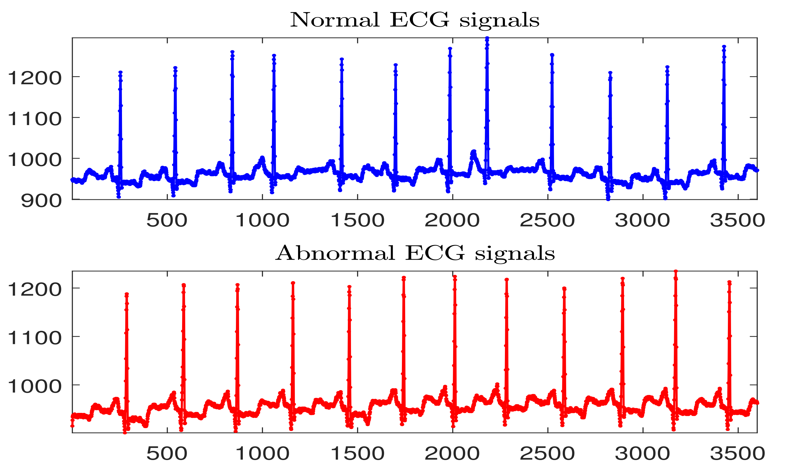
In this section, we consider applying the proposed method to real problems to verify whether MF-S-DFA is more efficient than conventional MF-DFA. We perform empirical analysis with ECG signals collected from the MIT-BIH arrhythmia database [29]. All data were sampled at a frequency of 360 Hz and a standard of 200 adu/mV, and each sample consisted of 3600 points. To ensure fairness in classification, 50 cases of normal ECG signals and 50 cases of abnormal ECG signals were selected. We use the generalized Hurst exponent H ( q ) extracted by MF-S-DFA and MF-DFA as the features of the ECG signals and then analyze them as input vectors of the support vector machine to compare the effectiveness of the two methods. Figure 10 shows a normal ECG signal and an abnormal ECG signal for 10 s.
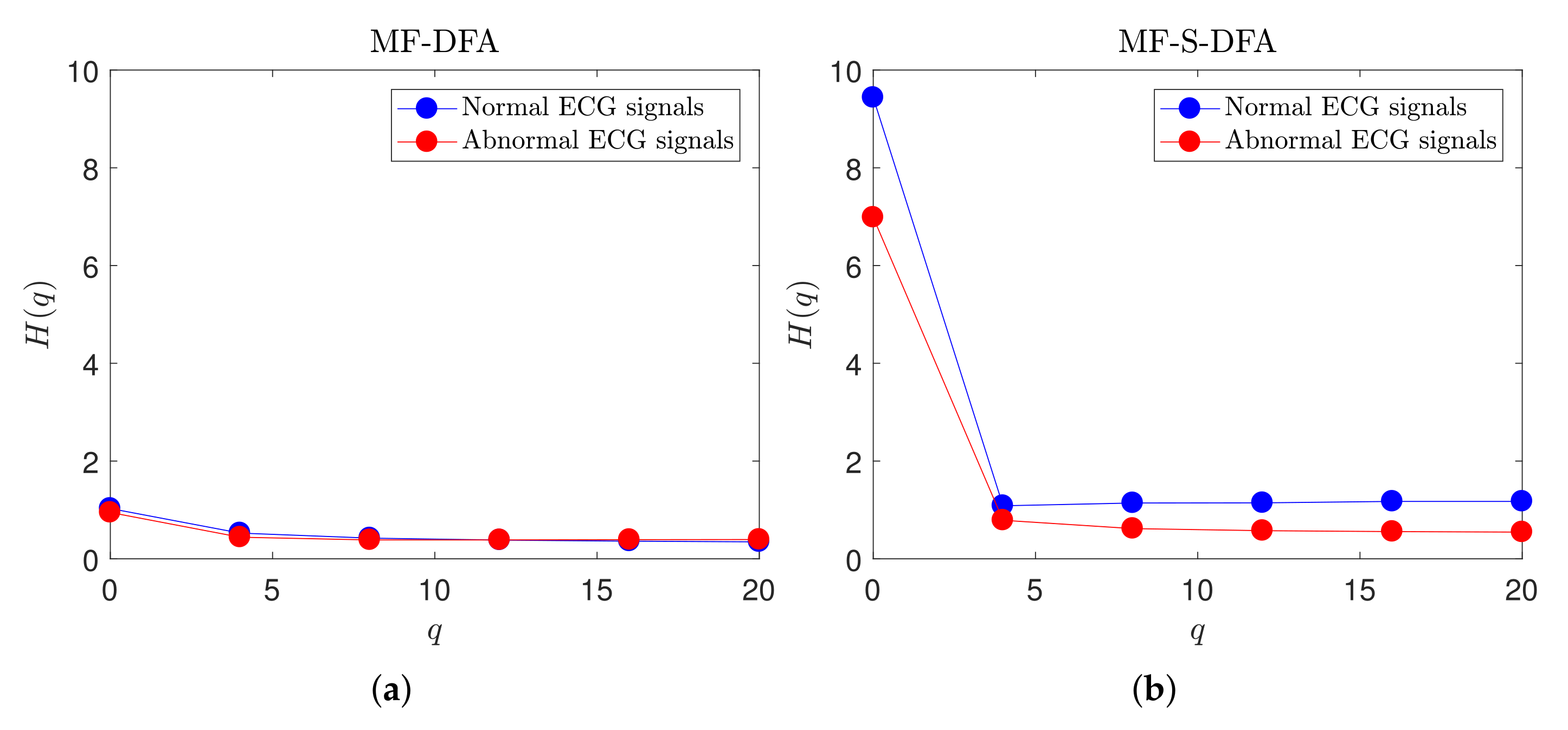
For feature extraction using MF-S-DFA and MF-DFA, we set the minimum segment size s m i n = 130 and the maximum segment size s m a x = 390, and the number of segments is 11 in total. We take the total number of q as 6, with the value between 0 and 20. As shown in Figure 11, the blue solid points represent normal ECG signals, and the red solid points represent abnormal ECG signals; (a) represents the generalized Hurst exponent H ( q ) by conventional MF-DFA; (b) represents the generalized Hurst exponent H ( q ) by MF-S-DFA. We fixed the x- and y-axis intervals of the two images. Obviously, compared with conventional MF-DFA, the generalized Hurst exponent extracted by MF-S-DFA shows a greater difference between normal ECG signals and abnormal ECG signals.
Afterwards, we use the obtained generalized Hurst exponent H ( q ) as the input vector for the support vector machine and put it into the SVM classifier for further verification. Accuracy, sensitivity and specificity were used to measure classification. The three indicators are calculated as follows.
Accuracy = TP + TN TP + FN + FP + TN ,
Sensitivity = TP TP + FN ,
Specificity = TN FP + TN ,
Among them, TP: abnormal marked as abnormal; FN: normal marked as abnormal; TN: normal marked as normal; FP: abnormal marked as normal.
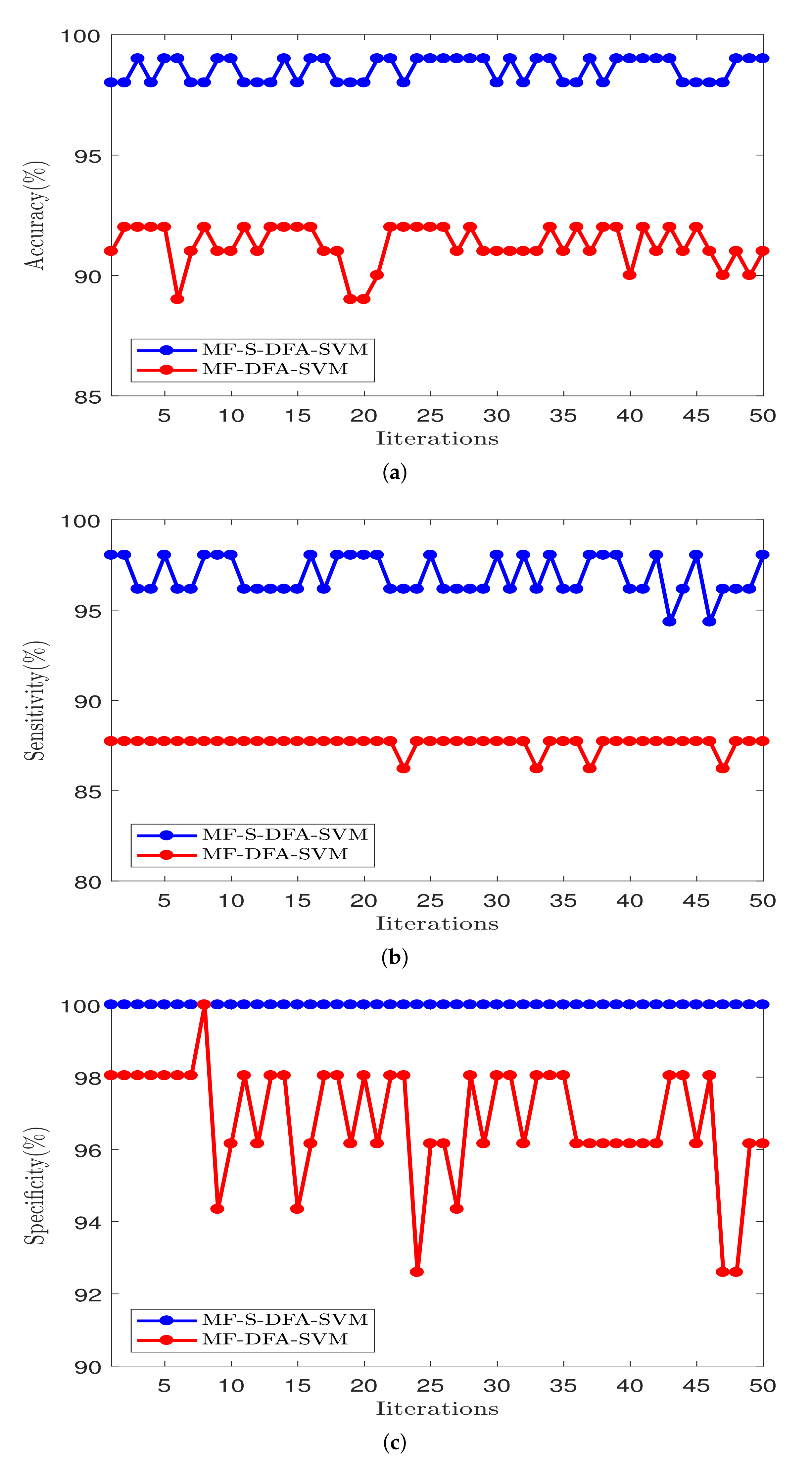
During classification, the SVM classifier uses a Gaussian kernel function and selects 90% of the dataset as the training set and 10% as the test set. We use k-fold cross-validation for classification validation, with k = 10, and calculate each classification evaluation index after 50 iterations. In Figure 12, the red line represents the classification evaluation index of MF-DFA-SVM, and the blue line represents the classification evaluation index of MF-S-DFA-SVM: (a) accuracy, (b) sensitivity and (c) specificity. It can be seen that the classification accuracy of the proposed MF-S-DFA is above 95%, while the classification accuracy of MF-DFA is far lower than 95%. In addition, the sensitivity and specificity of MF-DFA were higher than those of conventional MF-DFA. Therefore, classification by MF-S-DFA is superior to that by conventional MF-DFA.
In addition, we calculate the means and standard deviations of accuracy, sensitivity and specificity after 50 iterations, as shown in Table 4. The results show that accuracy, sensitivity and specificity of MF-S-DFA are significant in ECG signal classification. Compared with conventional MF-DFA, the proposed MF-S-DFA is more effective in practical applications.

5. Conclusions

In this paper, we proposed an MF-S-DFA algorithm based on conventional MF-DFA. The concept of the algorithm is to add sign retention into the MF-DFA algorithm to optimize the internal structure of classical MF-DFA. The results of various numerical experiments demonstrated that the proposed method can more effectively extract target features. Based on the p model, multiplication cascade time series were used to test the performance of the proposed MF-S-DFA. The generalized Hurst exponent H ( q ) , the scale exponent τ ( q ) and the singular spectrum f ( α ) were used to evaluate the performance of the proposed algorithm. It was concluded that, compared with conventional MF-DFA, the calculated values of MF-S-DFA were more consistent with the theoretical values. To further estimate the capabilities of the algorithm, we also compared H e r r ( q ) and τ e r r ( q ) , and the conclusions were consistent with the above. Subsequently, by changing the values of different parameters, n m a x , q and p, we compare d H e r r ( q ) and τ e r r ( q ) for MF-DFA and MF-S-DFA, and the optimized values were always more consistent with the theoretical values, which shows that processing non-stationary time series using MF-S-DFA can more accurately describe multi-fractal characteristics. Afterwards, we calculated distance function such as D H and D τ under different parameters and compared the performance of the two methods. The results indicated that MF-S-DFA has the lower error and provided better accuracy estimates, which indicated that MF-S-DFA using sign retention performed better than conventional MF-DFA. Besides, in ECG classification, we concluded that the proposed MF-S-DFA was more effective than conventional MF-DFA.

Author Contributions

Conceptualization, J.W. and M.Y.; methodology, J.W.; software, M.Y.; validation, M.Y., Y.Z. and J.W.; formal analysis, M.Y.; investigation, Y.Z.; resources, J.W.; data curation, M.Y.; writing—original draft preparation, M.Y.; writing—review and editing, J.W.; visualization, Y.Z.; supervision, J.W.; project administration, J.W.; funding acquisition, M.Y. and J.W. All authors have read and agreed to the published version of the manuscript.

Funding

The first author (Mengdie Yang) expresses thanks for the Jiangsu Graduate Research and Practice Innovation Plan in 2022 (SJCX22_0331). The corresponding author (Jian Wang) was supported by “The Startup Foundation for Introducing Talent of NUIST’, and Jiangsu Shuangchuang project (JSSCBS20210473).

Institutional Review Board Statement

Not applicable.

Informed Consent Statement

Not applicable.

Data Availability Statement

Not applicable.

Acknowledgments

The authors are grateful to the reviewers for their valuable suggestions and comments, which significantly improved the quality of this article.

Conflicts of Interest

The authors declare that there is no conflict of interests regarding the publication of this article.

References

  1. Xu, L.; Ivanov, P.C.; Hu, K.; Chen, Z.; Carbone, A.; Stanley, H.E. Quantifying signals with power-law correlations: A comparative study of detrended fluctuation analysis and detrended moving average techniques. Phys. Rev. E 2005, 71, 051101. [Google Scholar] [CrossRef] [PubMed] [Green Version]
  2. Jiang, Z.Q.; Xie, W.J.; Zhou, W.X.; Sornette, D. Multifractal analysis of financial markets: A review. Rep. Prog. Phys. 2019, 82, 125901. [Google Scholar] [CrossRef] [PubMed] [Green Version]
  3. Pratviel, Y.; Deschodt-Arsac, V.; Larrue, F.; Arsac, L.M. Tool Embodiment Is Reflected in Movement Multifractal Nonlinearity. Fractal Fract. 2022, 6, 240. [Google Scholar] [CrossRef]
  4. Wang, J.; Shao, W.; Kim, J. Automated classification for brain MRIs based on 2D MF-DFA method. Fractals 2020, 28, 2050109. [Google Scholar] [CrossRef]
  5. Kantelhardt, J.W.; Zschiegner, S.A.; Koscielny-Bunde, E.; Havlin, S.; Bunde, A.; Stanley, H.E. Multifractal detrended fluctuation analysis of nonstationary time series. Phys. A Stat. Mech. Its Appl. 2002, 316, 87–114. [Google Scholar] [CrossRef] [Green Version]
  6. Peng, C.K.; Buldyrev, S.V.; Havlin, S.; Simons, M.; Stanley, H.E.; Goldberger, A.L. Mosaic organization of DNA nucleotides. Phys. Rev. E. 1994, 49, 1685. [Google Scholar] [CrossRef] [Green Version]
  7. Podobnik, B.; Stanley, H.E. Detrended cross-correlation analysis: A new method for analyzing two nonstationary time series. Phys. Rev. Lett. 2008, 100, 084102. [Google Scholar] [CrossRef] [Green Version]
  8. Zhou, W.X. Multifractal detrended cross-correlation analysis for two nonstationary signals. Phys. Rev. E. 2008, 77, 066211. [Google Scholar] [CrossRef] [Green Version]
  9. Yuan, Y.; Zhuang, X.T.; Liu, Z.Y. Price—Volume multifractal analysis and its application in Chinese stock markets. Phys. A Stat. Mech. Its Appl. 2012, 391, 3484–3495. [Google Scholar] [CrossRef]
  10. Shao, W.; Wang, J. Does the “ice-breaking” of South and North Korea affect the South Korean financial market? Chaos Solitons Fractals 2020, 132, 109564. [Google Scholar] [CrossRef]
  11. Kim, K.; Yoon, S.M. Multifractal features of financial markets. Phys. A Stat. Mech. Its Appl. 2004, 344, 272–278. [Google Scholar] [CrossRef]
  12. Zhang, X.; Liu, H.; Zhao, Y.; Zhang, X. Multifractal detrended fluctuation analysis on air traffic flow time series: A single airport case. Phys. A Stat. Mech. Its Appl. 2019, 531, 121790. [Google Scholar] [CrossRef]
  13. Shang, P.; Lu, Y.; Kamae, S. Detecting long-range correlations of traffic time series with multifractal detrended fluctuation analysis. Chaos Solitons Fractals 2008, 36, 82–90. [Google Scholar] [CrossRef]
  14. Li, X.; Shang, P. Multifractal classification of road traffic flows. Chaos Solitons Fractals 2007, 31, 1089–1094. [Google Scholar] [CrossRef]
  15. Zhang, C.; Ni, Z.; Ni, L. Multifractal detrended cross-correlation analysis between PM2.5 and meteorological factors. Phys. A Stat. Mech. Its Appl. 2015, 438, 114–123. [Google Scholar] [CrossRef]
  16. Lee, C.K. Multifractal characteristics in air pollutant concentration time series. Water Air Soil Pollut. 2002, 135, 389–409. [Google Scholar] [CrossRef]
  17. Stan, C.; Cristescu, M.T.; Luiza, B.I.; Cristescu, C.P. Investigation on series of length of coding and non-coding DNA sequences of bacteria using multifractal detrended cross-correlation analysis. J. Theor. Biol. 2013, 321, 54–62. [Google Scholar] [CrossRef]
  18. Gutierrez, J.M.; Rodrıguez, M.A.; Abramson, G. Multifractal analysis of DNA sequences using a novel chaos-game representation. Phys. A Stat. Mech. Its Appl. 2001, 300, 271–284. [Google Scholar] [CrossRef]
  19. Mandal, S.; Sinha, N. Arrhythmia diagnosis from ECG signal analysis using statistical features and novel classification method. J. Mech. Med. Biol. 2021, 21, 2150025. [Google Scholar] [CrossRef]
  20. Wang, J.; Shao, W.; Kim, J. ECG Classification Comparison Between MF-DFA and MF-DXA. Fractals 2021, 29, 2150029. [Google Scholar] [CrossRef]
  21. Riedi, R. An improved multifractal formalism and self-similar measures. J. Math. Anal. Appl. 1995, 189, 462–490. [Google Scholar] [CrossRef] [Green Version]
  22. Wang, J.; Jiang, W.; Shao, W. Convergence investigation of multifractal analysis based on Lp-norm constraint. Fractals 2022. [Google Scholar] [CrossRef]
  23. Lee, Y.J.; Kim, N.W.; Choi, K.H.; Yoon, S.M. Analysis of the informational efficiency of the EU carbon emission trading market: Asymmetric MF-DFA approach. Energies 2020, 13, 2171. [Google Scholar] [CrossRef]
  24. Wang, J.; Shao, W. Multifractal analysis with detrending weighted average algorithm of historical volatility. Fractals 2021, 29, 2150193. [Google Scholar] [CrossRef]
  25. Lavicka, H.; Kracik, J. Fluctuation analysis of electric power loads in Europe: Correlation multifractality vs. Distribution function multifractality. Phys. A Stat. Mech. Its Appl. 2020, 545, 123821. [Google Scholar] [CrossRef] [Green Version]
  26. Sosa-Herrera, J.A.; Rodriguez-Romo, S. Kernel density approach to error estimation of MF-DFA measures on time series. Phys. A Stat. Mech. Its Appl. 2019, 526, 120863. [Google Scholar] [CrossRef]
  27. Meneveau, C.; Sreenivasan, K.R. Simple multifractal cascade model for fully developed turbulence. Phys. Rev. Lett. 1987, 59, 1424. [Google Scholar] [CrossRef]
  28. Halsey, T.C.; Jensen, M.H.; Kadanoff, L.P.; Procaccia, I.; Shraiman, B.I. Fractal measures and their singularities: The characterization of strange sets. Phys. Rev. A 1986, 33, 1141. [Google Scholar] [CrossRef]
  29. Moody, G.B.; Mark, R.G. The impact of the MIT-BIH arrhythmia database. IEEE Eng. Med. Biol. Mag. 2001, 20, 45–50. [Google Scholar] [CrossRef]
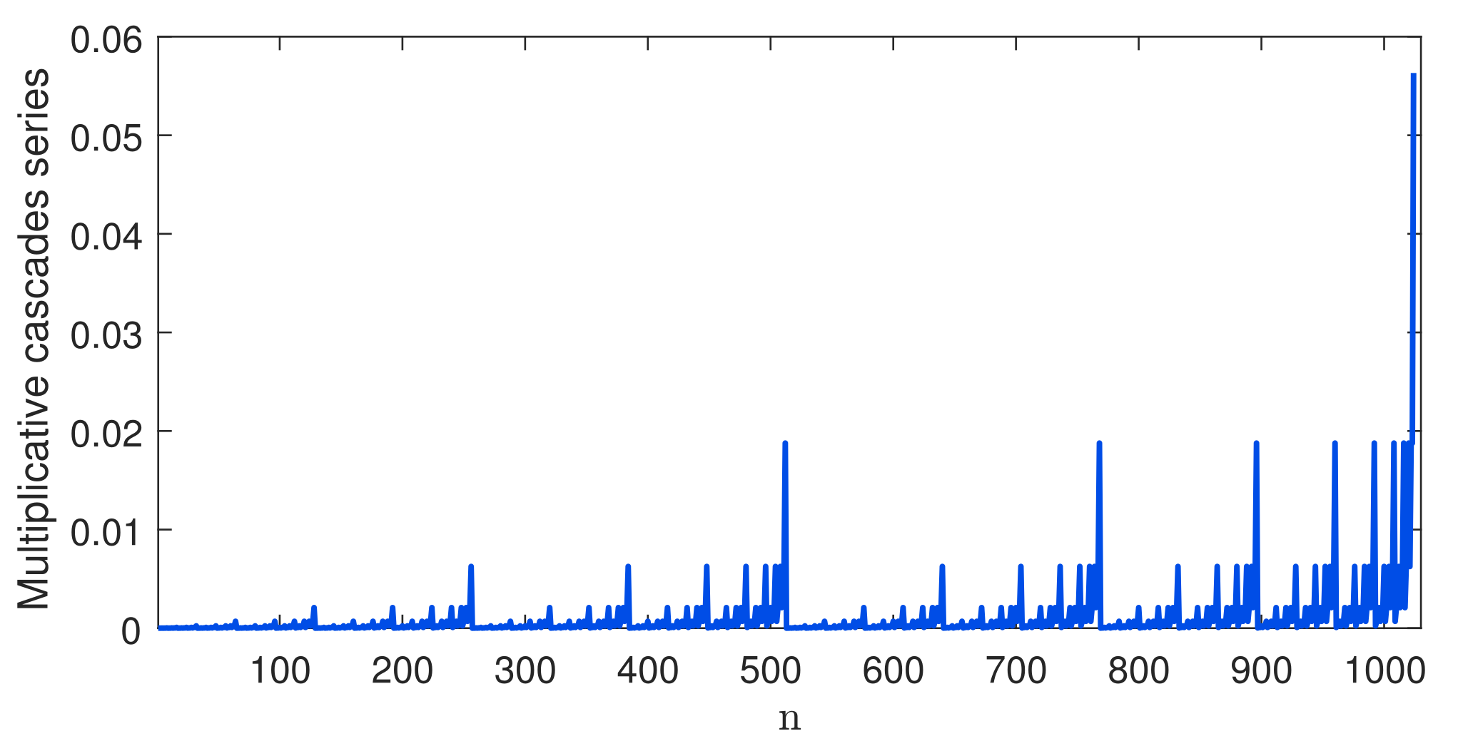
Figure 1. Multiplicative cascades series under p-model with p = 0.75 and n m a x = 10.
Fractalfract 06 00365 g001
Figure 2. (a) The time series. (b) Fitting the time series. (c) f v 2 ( s ) obtained with traditional MF-S-DFA. A color version of the figure is available in the web version of the article.
Fractalfract 06 00365 g002
Figure 3. Multifractal analysis of the constructed multiplicative cascade time series of (a) generalized Hurst exponent H ( q ) calculated by MF-DFA and MF-S-DFA and analytical value and (b) mass exponent spectrum τ ( q ) calculated by MF-DFA and MF-S-DFA and analytical value. A color version of the figure is available in the web version of the article.
Fractalfract 06 00365 g003
Figure 4. Multifractal analysis of the constructed multiplicative cascades time series comparison of the singular spectrum f ( α ) under different parameters n m a x . (af) represent n m a x = 8 , 9 , 10 , 11 , 12 and 13, respectively. A color version of the figure is available in the web version of the article.
Fractalfract 06 00365 g004
Figure 5. Multifractal analysis of the constructed multiplicative cascade time series: (a) relative error H e r r ( q ) of MF-DFA and MF-S-DFA algorithms, (b) relative error τ e r r ( q ) of MF-DFA and MF-S-DFA algorithms. A color version of the figure is available in the web version of the article.
Fractalfract 06 00365 g005
Figure 6. Comparison of MF-DFA and MF-S-DFA for different parameters of n m a x : (a) H e r r ( q ) and (b) τ e r r ( q ) . From top to bottom, n m a x = 8 , 9 , 10 , 11 , 12 and 13, respectively. A color version of the figure is available in the web version of the article.
Fractalfract 06 00365 g006aFractalfract 06 00365 g006b
Figure 7. Comparison of MF-DFA and MF-S-DFA with theoretical values under different domains of q: (a) H e r r ( q ) and (b) τ e r r ( q ) . From top to bottom, q = [ 5 , 5 ] , [ 10 , 10 ] , [ 15 , 15 ] , [ 20 , 20 ] , [ 25 , 25 ] and [ 30 , 30 ] , respectively. A color version of the figure is available in the web version of the article.
Fractalfract 06 00365 g007aFractalfract 06 00365 g007b
Figure 8. Comparison of MF-DFA and MF-S-DFA with theoretical values under different parameters p: (a) H e r r ( q ) and (b) τ e r r ( q ) . From top to bottom, p = 0.60 , 0.65 , 0.70 , 0.75 , 0.80 and 0.85 , respectively. A color version of the figure is available in the web version of the article.
Fractalfract 06 00365 g008aFractalfract 06 00365 g008b
Figure 9. The difference between D H and D τ for MF-DFA and MF-S-DFA at different parameters of p: (a) Δ D H and (b) Δ D τ .
Fractalfract 06 00365 g009
Figure 10. Normal and abnormal 10 s ECG segment. A color version of the figure is available in the web version of the article.
Fractalfract 06 00365 g010
Figure 11. Generalized Hurst exponent H ( q ) extracted by (a) MF-DFA and (b) MF-S-DFA. A color version of the figure is available in the web version of the article.
Fractalfract 06 00365 g011
Figure 12. Classification evaluation index: (a) accuracy, (b) sensitivity and (c) specificity. A color version of the figure is available in the web version of the article.
Fractalfract 06 00365 g012
Table 1. D H and D τ for two methods with different lengths of simulation data.
n max    8910111213
MF-DFA0.15500.15980.16350.15570.15660.1488
D H MF-S-DFA0.11800.08940.12470.10440.08700.0570
MF-DFA1.95391.98971.99711.95851.99701.9816
D τ MF-S-DFA0.65850.42780.52650.46610.59200.4746
Table 2. D H and D τ for two methods with different domains of q.
q    [ 5 , 5 ] [ 10 , 10 ] [ 15 , 15 ] [ 20 , 20 ] [ 25 , 25 ] [ 30 , 30 ]
MF-DFA0.15970.16250.16350.16350.16320.1629
D H MF-S-DFA0.15950.13930.12940.12470.12250.1213
MF-DFA0.49101.00021.50241.99712.48932.9811
D τ MF-S-DFA0.21290.30460.41390.52650.63970.7526
Table 3. D H and D τ for two methods with different values of p.
p    0.60 0.65 0.70 0.75 0.80 0.85
MF-DFA0.12930.10160.11290.16350.22590.2942
D H MF-S-DFA0.12980.09760.12140.12470.16080.1762
MF-DFA1.59951.16091.27811.99712.81433.6819
D τ MF-S-DFA1.32230.94300.70180.52651.21691.8197
Table 4. Classification evaluation metrics for MF-S-DFA-SVM and MF-DFA-SVM: accuracy, sensitivity and specificity.
MethodAccuracySensitivitySpecificity
MF-S-DFA-SVM 98.30 % ± 0.7618 96.95 % ± 0.1005 99.96 % ± 0.0527
MF-DFA-SVM 91.36 % ± 0.9227 87.54 % ± 0.0853 96.77 % ± 0.1207
Publisher’s Note: MDPI stays neutral with regard to jurisdictional claims in published maps and institutional affiliations.