The Oscillatory Flow of Oldroyd-B Fluid with Magnetic Disturbance

Abstract

The magnetic field intensity will be nondeterminacy with the flow of charged particles thrown out by solar activities, the overlap of adjacent magnetic islands or non-axisymmetric magnetic interference in tokamaks and so on. The model of a generalized Oldroyd-B fluid with fractional derivative under oscillating pressure gradient and magnetic field with some disturbance will be considered in this paper. The disturbance is regarded as the background noise of the system, and the model is described by a fractional stochastic differential equation. Time and space are discretized by L1, L2 schemes based on piecewise linear interpolation and the central difference quotient method. We demonstrate the effects of the amplitude and period of the oscillating pressure gradient, magnetic parameter, fractional parameters and noise on the velocity field, and two special cases are given.

1. Introduction

Fractional calculus is a generalization of classical integral calculus. In recent years, it has been widely used in diverse fields of science and engineering [1,2]. The main reason for using derivatives of fractional order in applications is that it can obtain the global connection with power-law kernel in time and space, and it provides a unique idea to describe the memory processes and inheritance properties of different substances. With the development of viscoelastic fluids [3,4,5,6], the fractional order operator is widely applied to them, which have attracted more and more attention in many fields such as academic, chemical and petrochemical industries. Some related works about the theoretical analysis and numerical simulation of fractional calculus equations are various, such as Laplace transform, Hankel transform, finite difference method, finite element method, spectral method and so on. Generally, the magnetic field has a stabilizing effect on instability, therefore, magnetohydrodynamic (MHD) has great value in science and industry. Recently, Shen et al. [7] studied MHD viscoelastic fluid with a heat source, which introduced the time-dependent fractional derivative in formulating the boundary layer equations, and obtained the numerical solution by using the finite difference method and L1 algorithm. Zhang et al. [8] studied the unsteady two-dimensional (2D) flow analysis of MHD fractional Maxwell fluid induced by variable pressure gradient, and used the implicit finite difference method to compare with the exact solution. Feng et al. [9] considered the finite element method for a 2D generalized Oldroyd-B fluid in a magnetic field on convex domains, which has a special time-space coupled derivative. However, the magnetic field intensity is not necessarily a constant, for instance, it may be variable in the interior of the earth. Due to the importance of variable magnetic fields in chemical engineering and geophysics, some scholars consider the dynamic behavior of viscoelastic fluid under a variable magnetic field [10,11].

Unfortunately, there are complex physical fields in the practical environment, and the magnetic field intensity may not be completely represented by several perfect curves. It may be disturbed by other factors, such as the flow of charged particles thrown out by solar activities, the overlap of adjacent magnetic islands and non-axisymmetric magnetic disturbance in tokamaks. Because of these disturbances, the behavior of material properties in random magnetic field has attracted more and more attention [12,13,14]. Although most papers ignore the possible randomness of magnetic field when discussing the dynamic behavior of MHD, some researchers have made some achievements in studying the model of fluid driven by random external force. Xu et al. [15] proved the global existence and uniqueness of a weak solution of stochastic time-space fractional incompressible Navier–Stokes equations driven by white noise. P.A. Razafimandimby [16] studied the stochastic equation describing the motions of 2D incompressible linear viscoelastic fluids subject to periodic boundary conditions and driven by random external forces. Manil T. Mohan [17] established the unique global solvability, the existence of a unique ergodic and strongly mixing invariant measure of the stochastic 2D viscoelastic fluid equations, which arises from the Oldroyd model for the non-Newtonian fluid flows perturbed by multiplicative Gaussian noise. There are many studies of fluid driven by random forces or disturbed by noise, refer to [18,19,20,21]. These articles prove the existence and uniqueness of solutions from the theoretical view, however, few papers use numerical methods to analyze viscoelastic fluids driven by random external force. The exact solution of the stochastic differential equation is too difficult to obtain, and the finite difference method [22,23,24] and finite element method [25,26] are simple and effective numerical methods.

In this paper, we regard the disturbance in the magnetic field as background noise and describe the model with a fractional stochastic differential equation. The model is numerically analyzed by L1, L2 formulas based on linear interpolation and central difference quotient method, and the influence of the relevant parameters on the velocity field is described graphically.

2. Mathematical Model

The oscillatory flow of Oldroyd-B fluid under the effect of a magnetic field with perturbations in a uniform rectangular duct is considered. The continuity and momentum equations for an incompressible fluid are:

$$\nabla \mathbf{V}=0.$$

(1)

and:

$$\rho (\frac{\mathrm{d}\mathbf{V}}{\mathrm{d}t}+(\mathbf{V}·\nabla )\mathbf{V})=-\nabla \mathbf{p}+\nabla ·\mathbf{S}+{\mathbf{F}}_b.$$

(2)

The dynamic behavior of a complex MHD between parallel plates does not always satisfy the classical law, and its mechanical evolution process has obvious memory effects. In many already published papers, fractional derivatives are widely used in the fluid model, and fit well with the experimental data of viscoelastic fluid [27,28]. The Laplace transformation of Riemann–Liouvile fractional derivative contains a fractional derivative term; however, the initial value of fractional order is difficult to obtain and the physical meaning is unclear in engineering. Therefore, the Caputo fractional derivative is often used in engineering and scientific applications [29,30]. The constitutive equation of fractional Oldroyd-B fluid is given as follows:

$$(1+{\lambda }^{\alpha }{\mathcal{D}}_t^{\alpha })\mathbf{S}=\mu (1+{\theta }^{\beta }{\mathcal{D}}_t^{\beta }){\mathbf{A}}_1.$$

(3)

where $\mathbf{V}$ is the fluid velocity, $\rho ,\mathbf{p},\mathbf{S}$ and ${\mathbf{F}}_b$ are the density of the fluid, the pressure, the extra stress tensor and the body force, respectively. $\mu ,\lambda ,\theta$ are material constants, which represent the viscosity coefficient, the relaxation and retardation times. ${\mathbf{A}}_1=\nabla \mathbf{V}+{(\nabla \mathbf{V})}^T$ is the first Rivlin–Ericksen tensor and ${\mathcal{D}}_t^{\alpha }\mathbf{S}$ and ${\mathcal{D}}_t^{\beta }{\mathbf{A}}_1$ are defined by:

$$\begin{array}{c}\hfill {\mathcal{D}}_t^{\alpha }\mathbf{S}=D_t^{\alpha }\mathbf{S}+(\mathbf{V}·\nabla )\mathbf{S}-(\nabla \mathbf{V})\mathbf{S}-\mathbf{S}{(\nabla \mathbf{V})}^{\mathbf{T}},\\ \hfill {\mathcal{D}}_t^{\beta }{\mathbf{A}}_1=D_t^{\beta }{\mathbf{A}}_1+(\mathbf{V}·\nabla ){\mathbf{A}}_1-(\nabla \mathbf{V}){\mathbf{A}}_1-{\mathbf{A}}_1{(\nabla \mathbf{V})}^{\mathbf{T}}.\end{array}$$

(4)

$D_t^{\alpha }$, and $D_t^{\beta }$ are the Caputo time-fractional derivatives of arbitrary order $\alpha ,\beta$. Caputo fractional derivative of order $\alpha >0$ for a function $f:(0,\infty )\to R$ can be written as [31]:

$$D_t^{\alpha }f\left(t\right)=\frac{\mathbf{1}}{\mathsf{\Gamma }(n-\alpha )}{\int }_0^t{(t-s)}^{n-\alpha -1}{f}^n\left(s\right)ds.$$

(5)

where $0\le n-1<\alpha <n$. It should be noted that when $\alpha =\beta =1$. Equation (3) is simplified as the ordinary Oldroyd-B model and when $\theta =0$. Equation (3) is simplified as the fractional Maxwell model.

For the unidirectional flow of the fractional Oldroyd-B fluid in the horizontal rectangular pipe, the velocity field is:

$$\mathbf{V}(u,v,w)=\left[u\right(y,z,t),0,0].$$

(6)

Furthermore, we consider that the fluid is permeated by a non-uniform magnetic field $(B_0+ϵ,0,0)$, $B_0$ is the deterministic magnetic field intensity, $ϵ$ is a perturbation factor of the system, which applies in the positive y-direction. $\sigma {(B_0+ϵ)}^2$ represents the magnetic body force in a low magnetic Reynolds number and $\sigma$ represents the electrical conductivity of the fluid. The momentum equation with the pressure gradient in the x-direction is:

$$\begin{array}{cc}\hfill (1+{\lambda }^{\alpha }{D}_t^{\alpha })\frac{\partial u}{\partial t}=& \nu (1+{\theta }^{\beta }{D}_t^{\beta })(\Delta u)-\frac{1}{\rho }(1+{\lambda }^{\alpha }{D}_t^{\alpha })\frac{\partial \mathbf{p}}{\partial x}\hfill \\ \hfill & -\frac{\sigma }{\rho }(1+{\lambda }^{\alpha }{D}_t^{\alpha })u{(B_0+ϵ)}^2.\hfill \end{array}$$

(7)

where $\nu =\frac{\mu }{\rho }$ is the kinematical viscosity, and $\Delta$ is the Laplace operator, $\Delta u=\frac{{\partial }^{2}u(y,z,t)}{{\partial }^2{y}^2}+\frac{{\partial }^{2}u(y,z,t)}{{\partial }^2{z}^2}$. It is provided that the pressure is $\frac{1}{\rho }\frac{\partial \mathbf{p}}{\partial x}=-kcos\left(\omega t\right)$, which is a harmonic periodic. $k,\omega$ are constants, which represent the amplitude and periodic parameters of the pressure gradient. Combined with Equation (7), we obtain:

$$(1+{\lambda }^{\alpha }{D}_t^{\alpha })\frac{\partial u}{\partial t}=\nu (1+{\theta }^{\beta }{D}_t^{\beta })(\Delta u)-M(1+{\lambda }^{\alpha }{D}_t^{\alpha })u+g(u,ϵ)+f(y,z,t).$$

(8)

where $M=\frac{\sigma B_0^2}{\rho }$ is a magnetic parameter, and $f(y,z,t)=kcos\left(\omega t\right)+k{\omega }^{\alpha }cos(\omega t+\frac{\alpha \pi }{2})$. We regard the term with disturbance as the noise of the background field, which is usually represented by addictive noise. Using a stochastic differential equation to describe this situation:

$$(1+{\lambda }^{\alpha }{D}_t^{\alpha })\frac{\partial u}{\partial t}=\nu (1+{\theta }^{\beta }{D}_t^{\beta })(\Delta u)-M(1+{\lambda }^{\alpha }{D}_t^{\alpha })u+f(y,z,t)+\xi \frac{dW}{dt}.$$

(9)

where $\xi$ is a constant, which denotes the intensity of noise. W is a standard Wiener process defined on a filtered probability space $(\mathsf{\Omega },\mathcal{F},{\mathcal{F}}_t,\mathcal{P})$ [32]. In this paper, the initial and boundary conditions are follows:

$$\begin{array}{c}\hfill u(y,z,0)={\mathsf{\Phi }}_1(y,z),u_t(y,z,0)={\mathsf{\Phi }}_2(y,z),0\le y\le L_1,0\le z\le L_2.\\ \hfill u(0,z,t)=0,u(L_1,z,t)=0,u(y,0,t)=0,u(y,L_2,t)=0,0<t\le T.\end{array}$$

(10)

where $L_1,L_2,T$ are constants, ${\mathsf{\Phi }}_1,{\mathsf{\Phi }}_2$ are known functions.

3. Numerical Discretization

The space $(y,z)\in [0,L_1]\times [0,L_2]$ are uniformly divided into $M_1\times M_2$ grids. Let $y_i=i{h}_1,z_j=j{h}_2,i=0,1,\cdots ,M_1,j=0,1,\cdots ,M_2$, where $h_1=\frac{L_1}{M_1}$ and $h_2=\frac{L_2}{M_2}$ are space steps in the y and z direction, respectively. Then, we divide the time into N grids, let $\tau =\frac{T}{N}$ be the time step and $t_n=n\tau ,n=0,1,\cdots ,N$.

Denote:

$u_{ij}^n=u(x_i,y_j,t_n),f_{ij}^n=f(x_i,y_j,t_n),W^n=W\left(t_n\right)$, $u_{ij}^{n-\frac{1}{2}}=\frac{u_{ij}^n+u_{ij}^{n-1}}{2},f_{ij}^{n-\frac{1}{2}}=\frac{f_{ij}^n+f_{ij}^{n-1}}{2}.$

${\delta }_t{u}_{ij}^n=\frac{u_{ij}^n-u_{ij}^{n-1}}{\tau },$${\delta }_y^2{u}_{ij}^n=\frac{u_{i+1,j}^n-2u_{ij}^n+u_{i-1,j}^n}{h_1^2},{\delta }_z^2{u}_{ij}^n=\frac{u_{i,j+1}^n-2u_{ij}^n+u_{i,j-1}^n}{h_2^2},{\delta }_t{W}^n=\frac{W^n-W^{n-1}}{\tau }$.

The implicit difference scheme of Crank–Nicolson is used to discretize on the time layer of $n-\frac{1}{2}$:

$$\begin{array}{cc}\hfill (1+{\lambda }^{\alpha }{D}_t^{\alpha })\frac{\partial u_{ij}^{n-\frac{1}{2}}}{\partial t}=& \nu (1+{\theta }^{\beta }{D}_t^{\beta })(\Delta u_{ij}^{n-\frac{1}{2}})-M(1+{\lambda }^{\alpha }{D}_t^{\alpha })u_{ij}^{n-\frac{1}{2}}\hfill \\ \hfill & +f(y_i,z_j,t_{n-\frac{1}{2}})+\xi \frac{d{W}^{n-\frac{1}{2}}}{dt}.\hfill \end{array}$$

(11)

Note $\gamma =1+\alpha ,1<\gamma <2$, the L1, L2 formulas based on piecewise linear interpolation are used, then:

$$\begin{array}{cc}\hfill D_t^{\alpha }{u}_{ij}^{n-\frac{1}{2}}=& \frac{D_t^{\alpha }{u}_{ij}^n+D_t^{\alpha }{u}_{ij}^{n-1}}{2}\hfill \\ \hfill =& \frac{{\tau }^{-\alpha }}{2\mathsf{\Gamma }(2-\alpha )}(a_0^{\left(\alpha \right)}{u}_{ij}^n-\sum _{k=1}^{n-1}(a_{n-k-1}^{\left(\alpha \right)}-a_{n-k}^{\left(\alpha \right)})u_{ij}^k-a_{n-1}^{\left(\alpha \right)}{u}_{ij}^0\hfill \\ \hfill & +a_0^{\left(\alpha \right)}{u}_{ij}^{n-1}-\sum _{k=1}^{n-2}(a_{n-k-2}^{\left(\alpha \right)}-a_{n-k-1}^{\left(\alpha \right)})u_{ij}^k-a_{n-2}^{\left(\alpha \right)}{u}_{ij}^0)+R_1\hfill \\ \hfill =& \frac{{\tau }^{1-\alpha }}{2\mathsf{\Gamma }(2-\alpha )}(\sum _{k=1}^n{a}_{n-k}^{\left(\alpha \right)}{\delta }_t{u}_{ij}^k+\sum _{k=1}^{n-1}{a}_{n-k-1}^{\left(\alpha \right)}{\delta }_t{u}_{ij}^k)+R_1\hfill \end{array}$$

(12)

where $|R_1|<C{\tau }^{(2-\alpha )}$.

$$\begin{array}{cc}\hfill D_t^{\gamma }{u}_{ij}^{n-\frac{1}{2}}=& \frac{D_t^{\gamma }{u}_{ij}^n+D_t^{\gamma }{u}_{ij}^{n-1}}{2}=\frac{{\tau }^{1-\gamma }}{\mathsf{\Gamma }(3-\gamma )}\hfill \\ \hfill & (a_0^{\left(\gamma \right)}{\delta }_t{u}_{ij}^n-\sum _{k=1}^{n-1}(a_{n-k-1}^{\left(\gamma \right)}-a_{n-k}^{\left(\gamma \right)}){\delta }_t{u}_{ij}^k-a_{n-1}^{\left(\gamma \right)}{\left(u_t\right)}_{ij}^0)+R_2\hfill \end{array}$$

(13)

where $|R_2|<C{\tau }^{(3-\gamma )}$.

Similarly, we have:

$$\begin{array}{cc}\hfill D_t^{\beta }{u}_{ij}^{n-\frac{1}{2}}& =\frac{D_t^{\beta }{u}_{ij}^n+D_t^{\beta }{u}_{ij}^{n-1}}{2}\hfill \\ \hfill & =\frac{{\tau }^{1-\beta }}{2\mathsf{\Gamma }(2-\beta )}(\sum _{k=1}^n{a}_{n-k}^{\left(\beta \right)}{\delta }_t{u}_{ij}^k+\sum _{k=1}^{n-1}{a}_{n-k-1}^{\left(\beta \right)}{\delta }_t{u}_{ij}^k)+R_3\hfill \end{array}$$

(14)

where $|R_3|<C{\tau }^{(2-\beta )}$.

As for the Laplace operator, $\Delta u^{n-\frac{1}{2}}=\frac{\Delta u_{ij}^n+\Delta u_{ij}^{n-1}}{2}=\frac{{\delta }_y^2{u}_{ij}^n+{\delta }_z^2{u}_{ij}^n+{\delta }_y^2{u}_{ij}^{n-1}+{\delta }_z^2{u}_{ij}^{n-1}}{2}$, and:

$$\begin{array}{cc}\hfill D_t^{\beta }\Delta u_{ij}^{n-\frac{1}{2}}=& \frac{{\tau }^{1-\beta }}{2\mathsf{\Gamma }(2-\beta )}(\sum _{k=1}^n{a}_{n-k}^{\left(\beta \right)}{\delta }_t({\delta }_y^2{u}_{ij}^k+{\delta }_z^2{u}_{ij}^k)\hfill \\ \hfill & +\sum _{k=1}^{n-1}{a}_{n-k-1}^{\left(\beta \right)}{\delta }_t({\delta }_y^2{u}_{ij}^k+{\delta }_z{u}_{ij}^k))+R_4\hfill \end{array}$$

(15)

where $|R_4|<C{\tau }^{(2-\beta )}$.

The coefficient $a_l^{\theta }$ is:

$$a_l^{\theta }=\left\{\begin{array}{c}{(l+1)}^{1-\theta }-l^{1-\theta },0<\theta <1\hfill \\ {(l+1)}^{2-\theta }-l^{2-\theta },1<\theta <2\hfill \end{array}l=0,1,\cdots ,N-1.\right.$$

(16)

Then central finite difference formula is used to approximate $\frac{d{W}^{n-\frac{1}{2}}}{dt}$:

$$\frac{d{W}^{n-\frac{1}{2}}}{dt}\approx \frac{W^n-W^{n-1}}{\tau }={\delta }_t{W}^n,n=1,2,\cdots ,N$$

(17)

Applying the Wiener process, $W\left(t_n\right)-W\left(t_{n-1}\right)\sim N(0,t_n-t_{n-1})$. That is, $\frac{W^n-W^{n-1}}{\sqrt{\tau }}\sim N(0,1)$. Omitting the small quantity term $R_i,i=1,\cdots ,4$, we get the following difference equation in this paper:

$$\begin{array}{cc}\hfill & {\lambda }^{\alpha }\frac{{\tau }^{1-\gamma }}{\mathsf{\Gamma }(3-\gamma )}(a_0^{\left(\gamma \right)}{\delta }_t{u}_{ij}^n-\sum _{k=1}^{n-1}(a_{n-k-1}^{\left(\gamma \right)}-a_{n-k}^{\left(\gamma \right)}){\delta }_t{u}_{ij}^k-a_{n-1}^{\left(\gamma \right)}{\left(u_t\right)}_{ij}^0)+{\delta }_t{u}_{ij}^n\hfill \\ \hfill & +M{\lambda }^{\alpha }\frac{{\tau }^{1-\alpha }}{2\mathsf{\Gamma }(2-\alpha )}(\sum _{k=1}^n{a}_{n-k}^{\left(\alpha \right)}{\delta }_t{u}_{ij}^k+\sum _{k=1}^{n-1}{a}_{n-k-1}^{\left(\alpha \right)}{\delta }_t{u}_{ij}^k)+M\frac{u_{ij}^n+u_{ij}^{n-1}}{2}\hfill \\ \hfill & -\nu \frac{{\delta }_y^2{u}_{ij}^n+{\delta }_z^2{u}_{ij}^n+{\delta }_y^2{u}_{ij}^{n-1}+{\delta }_z^2{u}_{ij}^{n-1}}{2}-\nu {\theta }^{\beta }\frac{{\tau }^{1-\beta }}{2\mathsf{\Gamma }(2-\beta )}\hfill \\ \hfill & (\sum _{k=1}^n{a}_{n-k}^{\left(\beta \right)}{\delta }_t({\delta }_y^2{u}_{ij}^k+{\delta }_z^2{u}_{ij}^k)+\sum _{k=1}^{n-1}{a}_{n-k-1}^{\left(\beta \right)}{\delta }_t({\delta }_y^2{u}_{ij}^k+{\delta }_z{u}_{ij}^k))\hfill \\ \hfill =& \frac{f_{ij}^n+f_{ij}^{n-1}}{2}+\xi {\delta }_t{W}^n.\hfill \end{array}$$

(18)

The initial and boundary conditions are discretized into:

$$\begin{array}{cc}\hfill u_{ij}^0={\mathsf{\Phi }}_1& (y_i,z_j),{\left(u_t\right)}_{ij}^0={\mathsf{\Phi }}_2(y_i,z_j),i=0,1,\cdots ,M_1,j=0,1,\cdots ,M_2.\hfill \\ & u_{0j}^n=u_{M_{1}j}^n=u_{i0}^n=u_{i{M}_2}^n=0,n=0,1,\cdots ,N.\hfill \end{array}$$

(19)

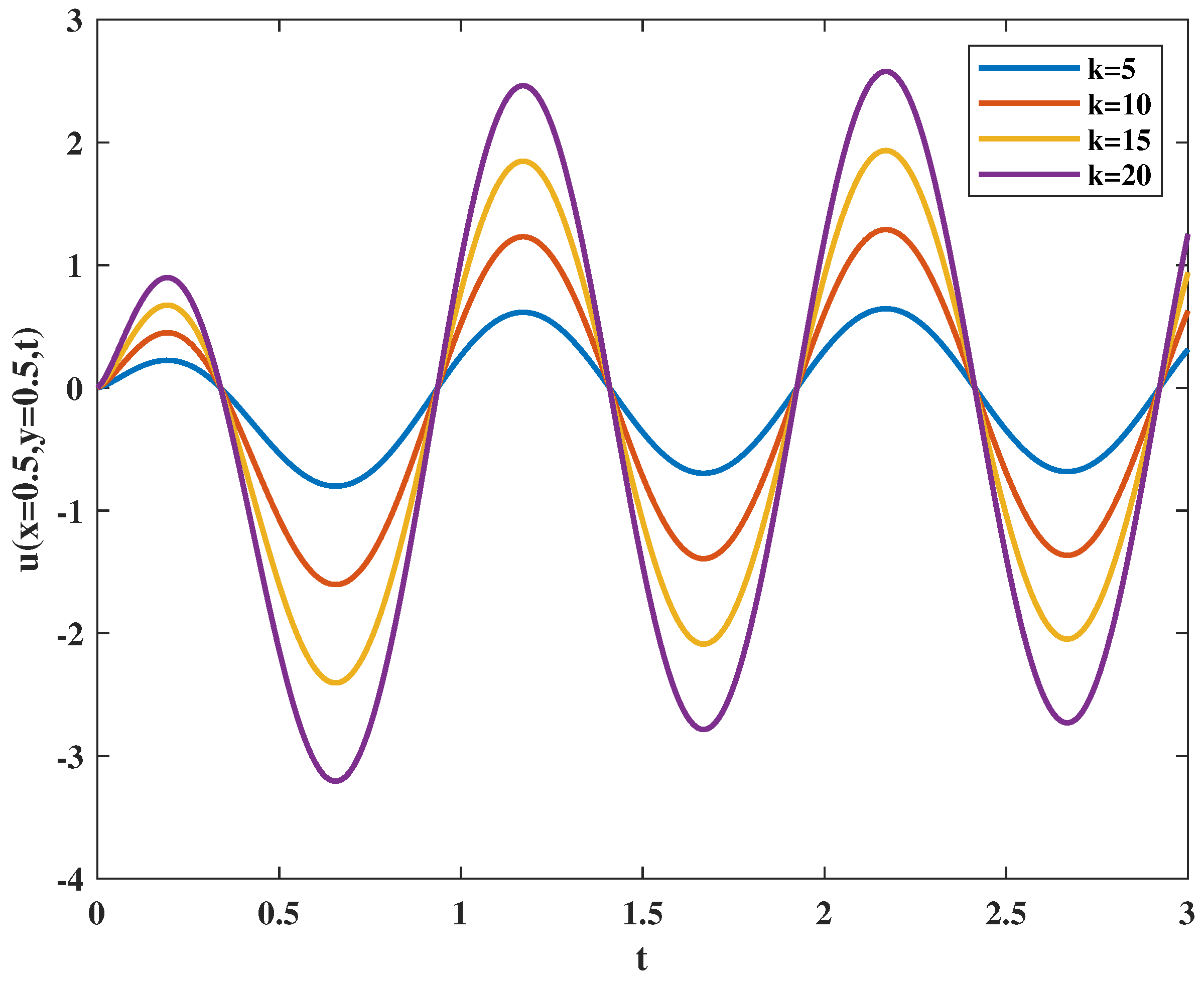
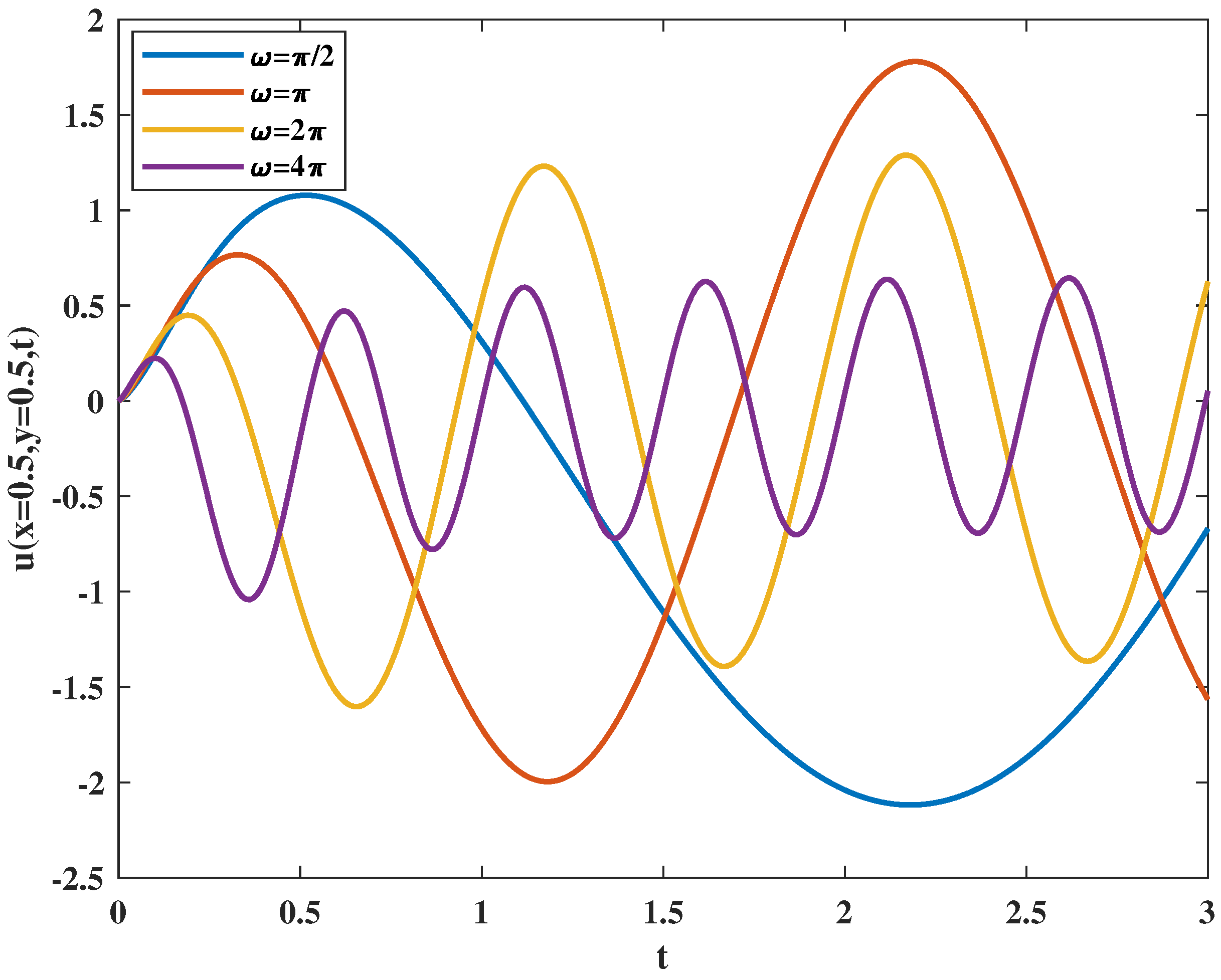
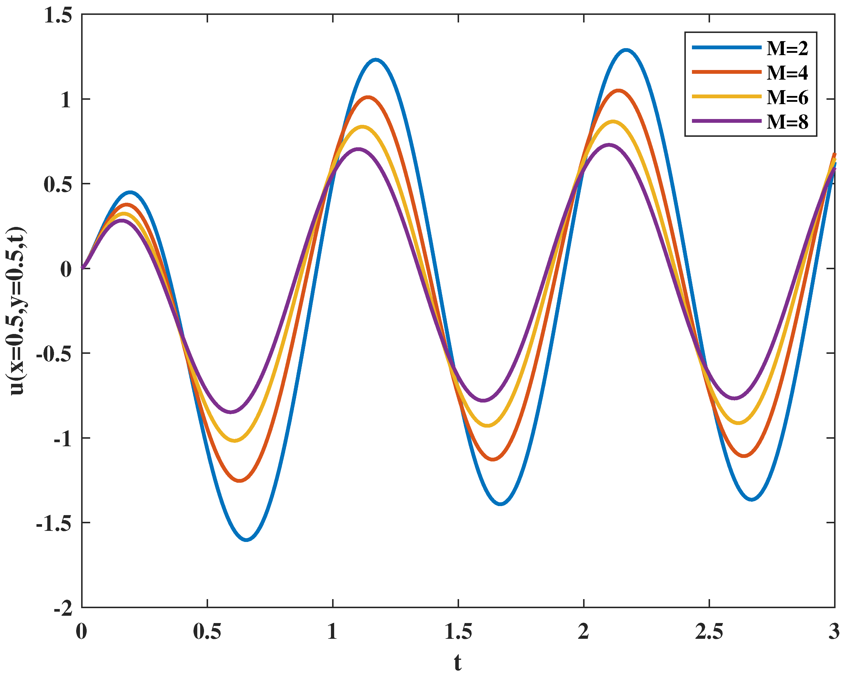
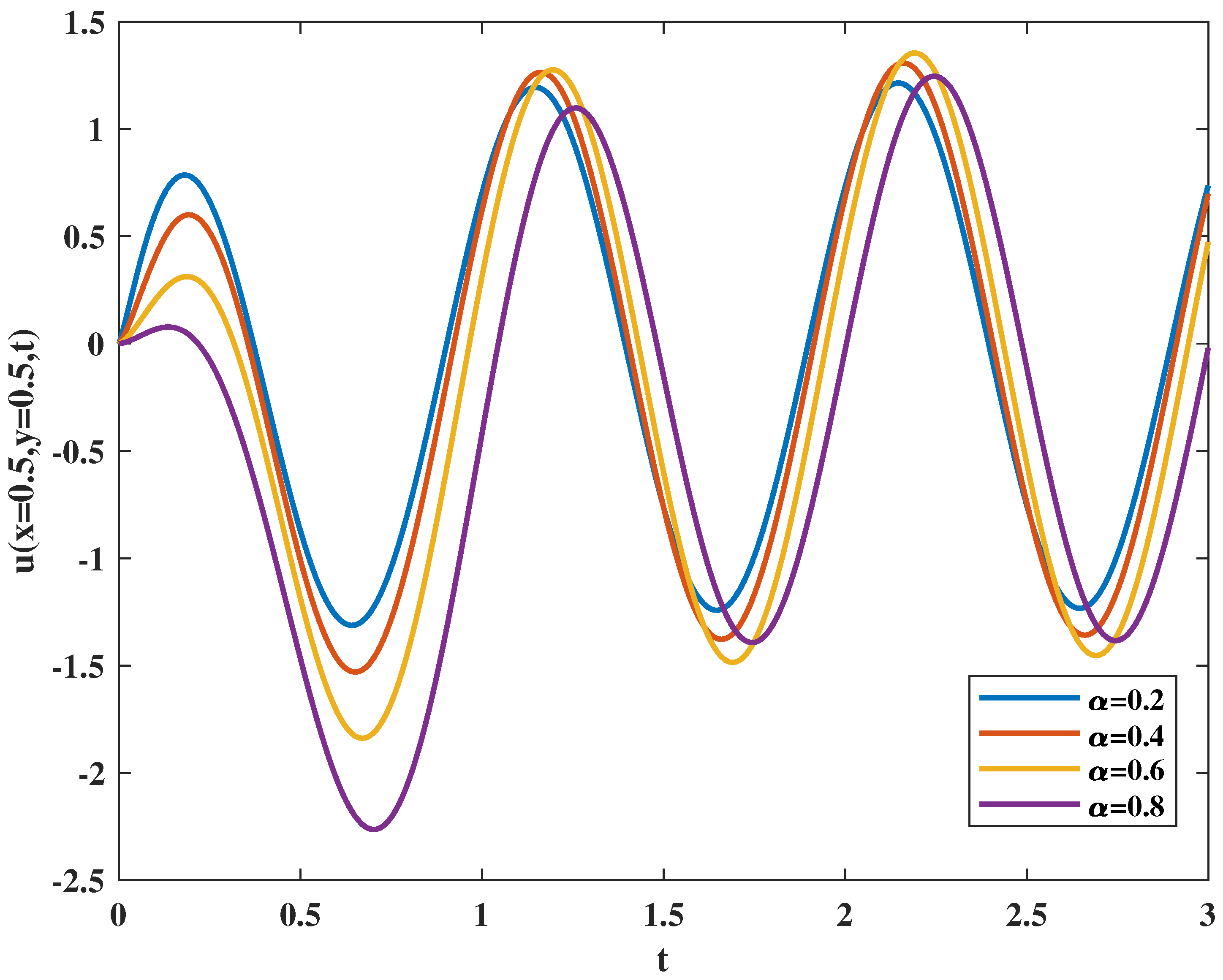
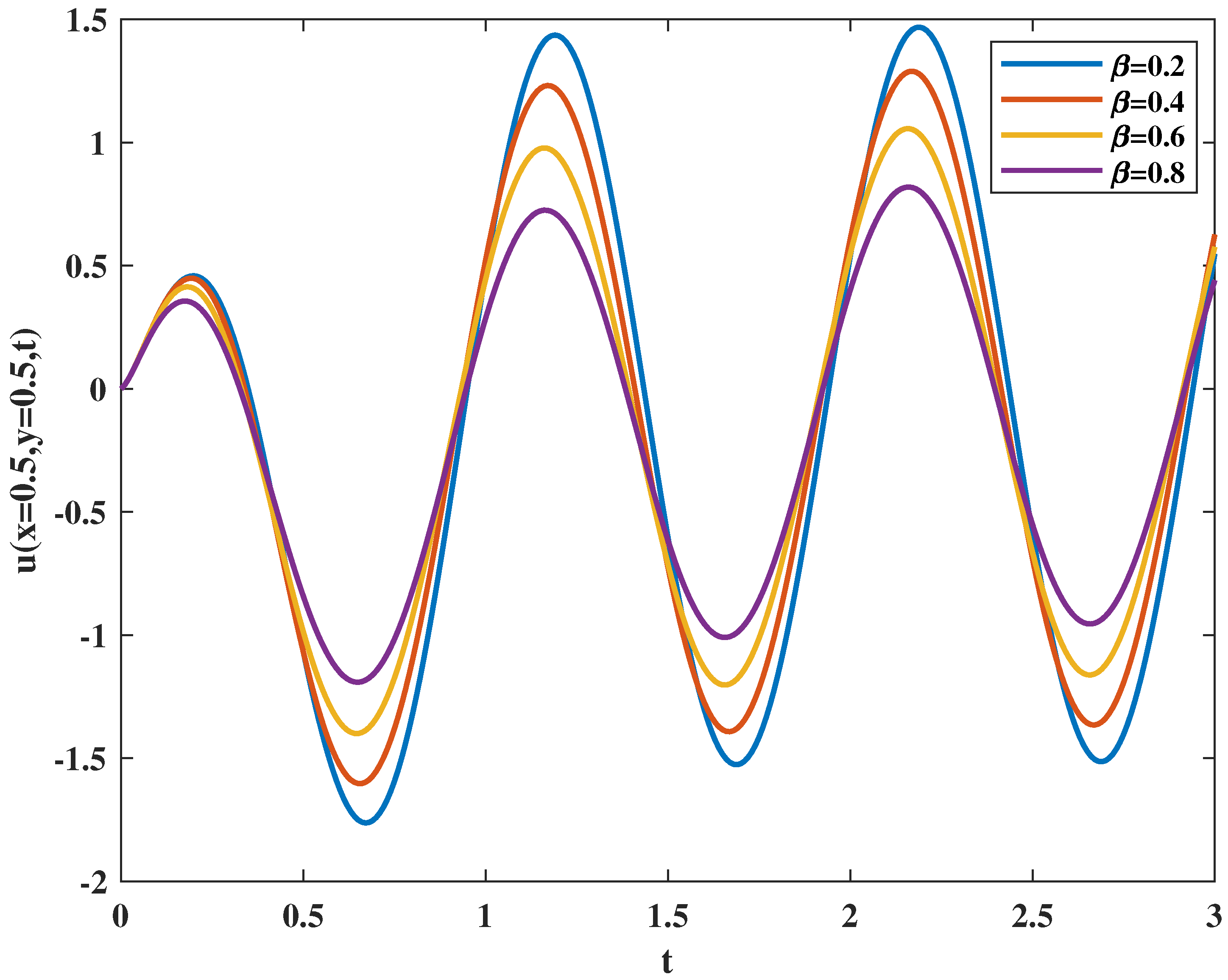
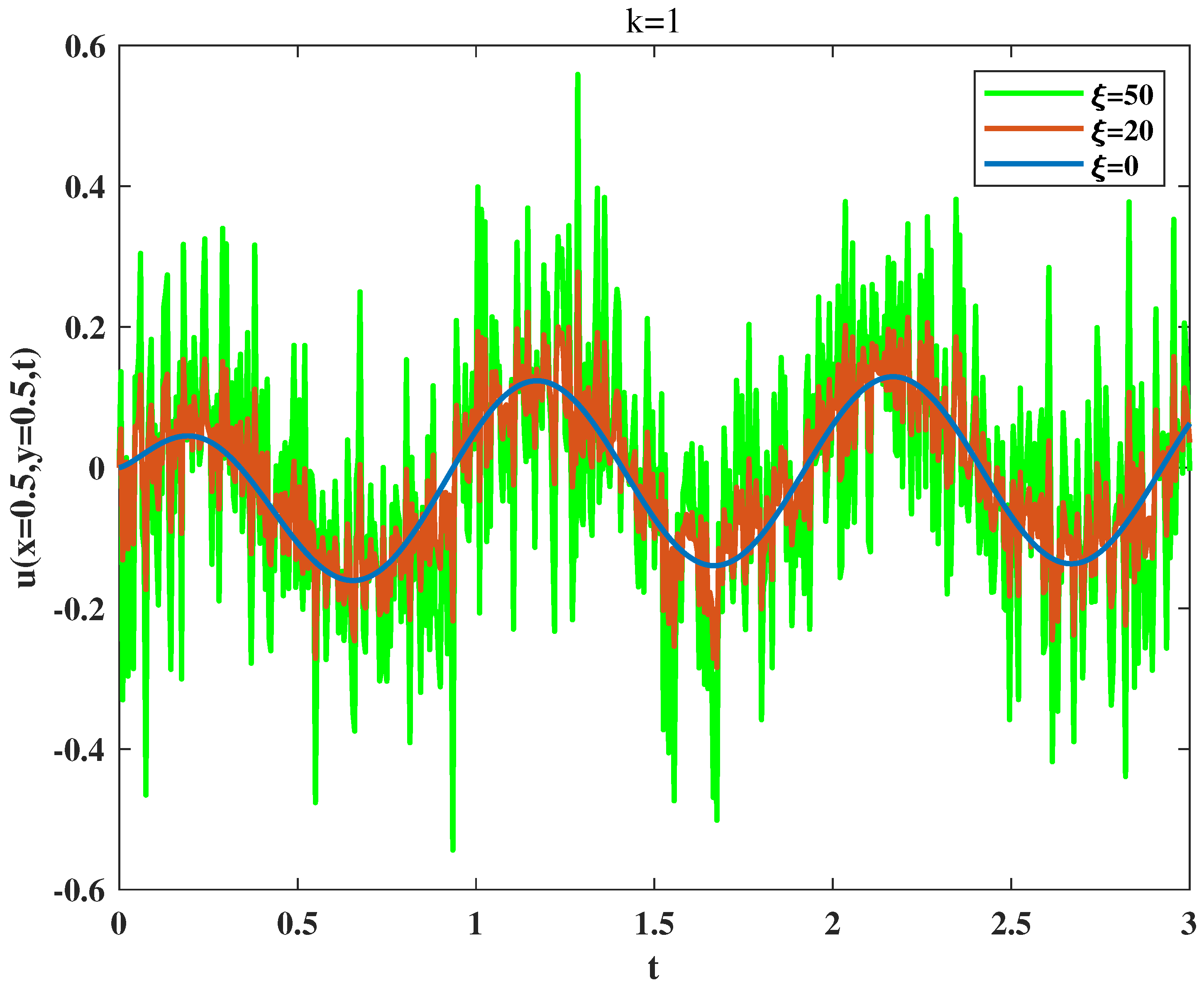
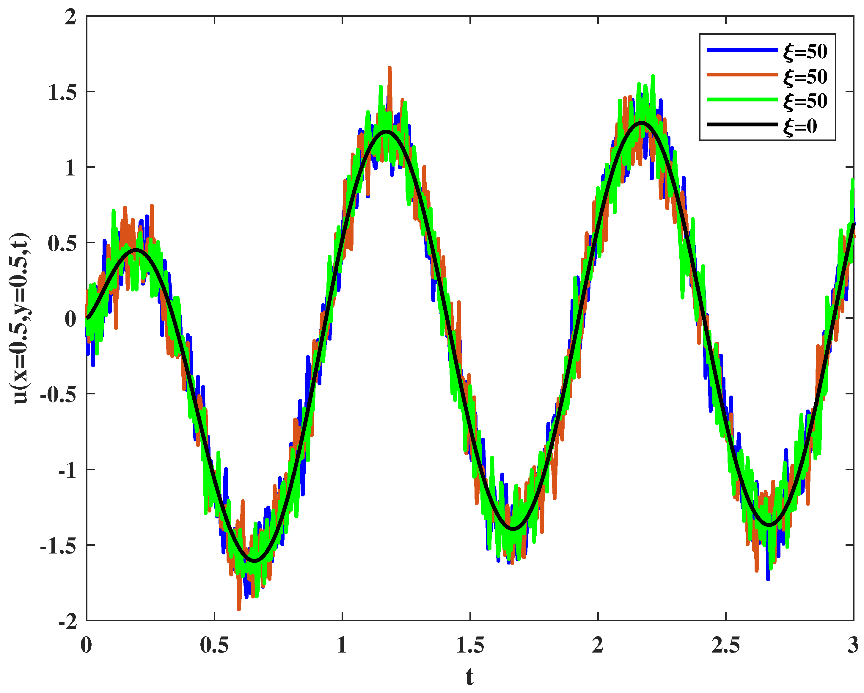
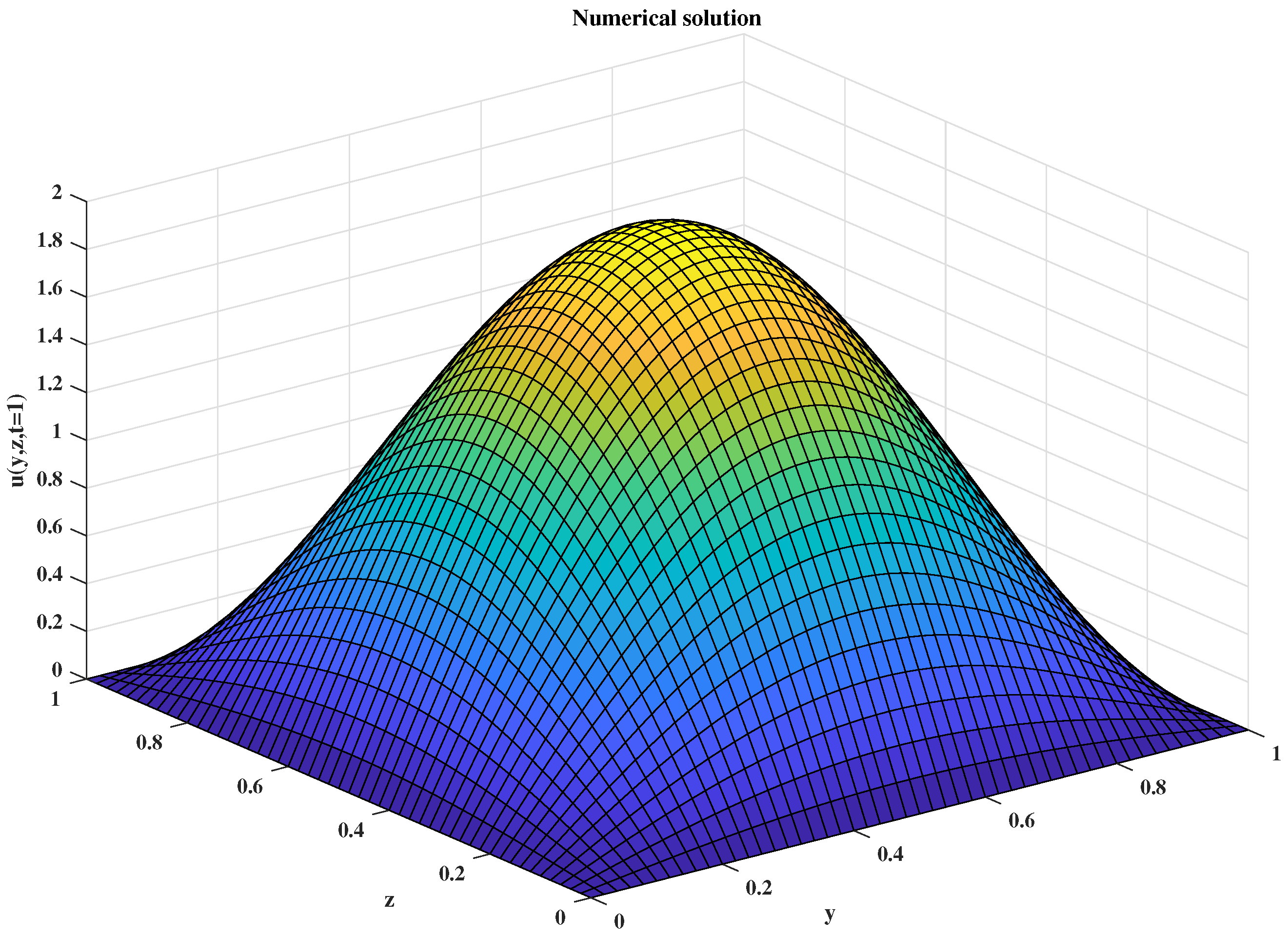
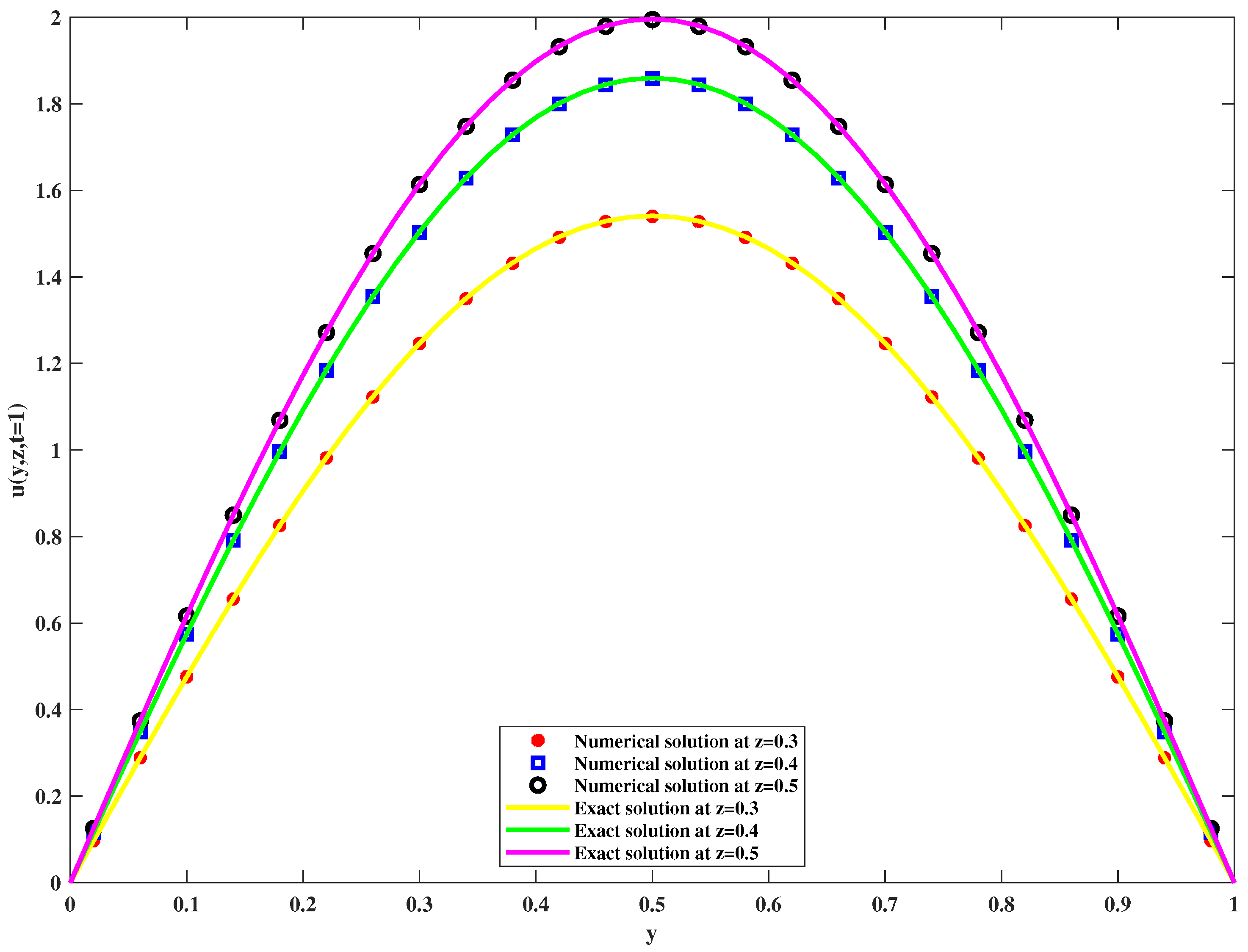
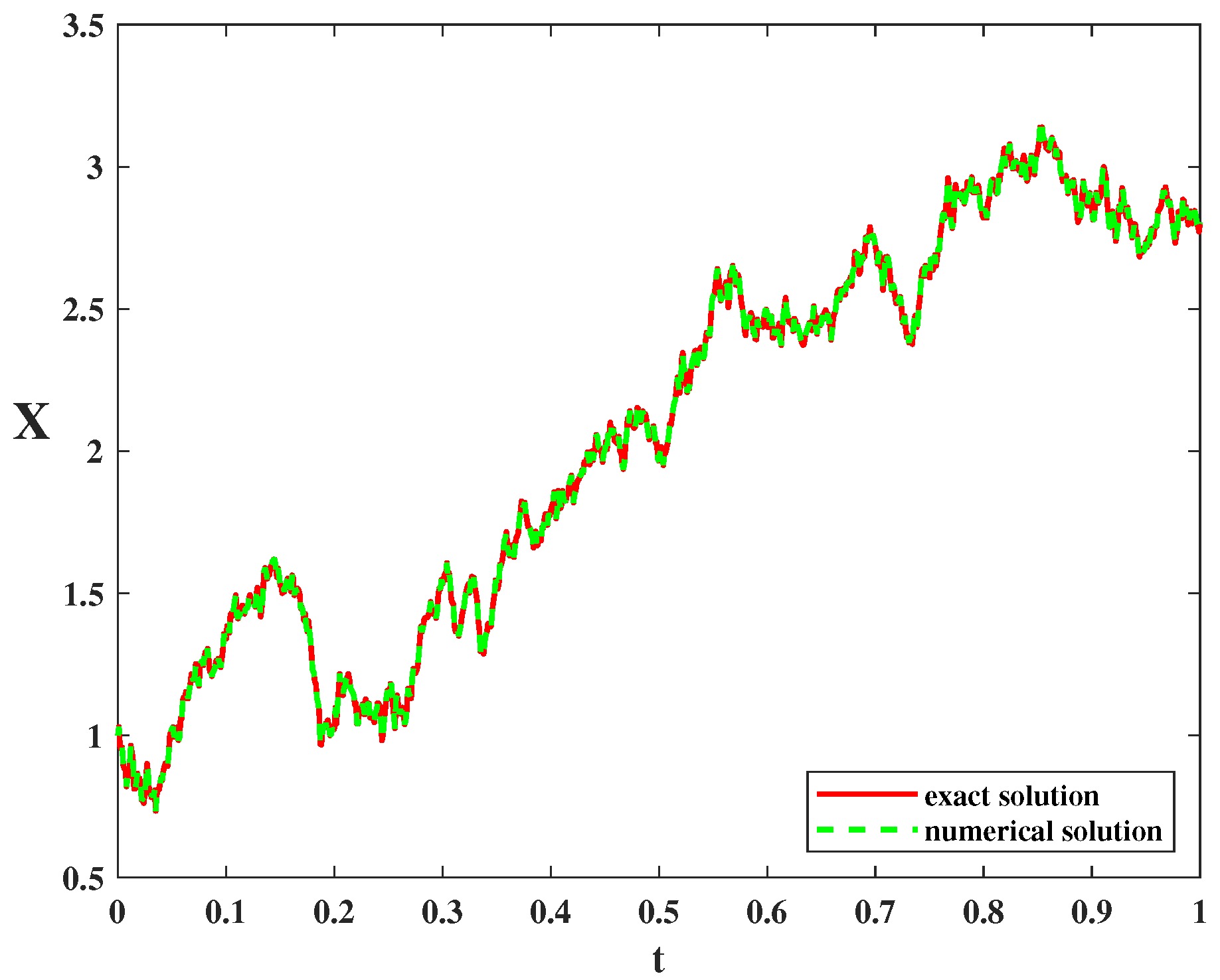
4. Results and Discussion

Oldroyd-B fluid with oscillating pressure gradient, magnetic field and addictive noise is considered:

$$\begin{array}{cc}\hfill & (1+{\lambda }^{\alpha }{D}_t^{\alpha })\frac{\partial u}{\partial t}=\nu (1+{\theta }^{\beta }{D}_t^{\beta })(\Delta u)-M(1+{\lambda }^{\alpha }{D}_t^{\alpha })u+f(y,z,t)+\xi \frac{dW}{dt}\hfill \\ \hfill & u(y,z,0)=0,u_t(y,z,0)=0,0\le y\le 1,0\le z\le 1.\hfill \\ \hfill & u(0,z,t)=0,u(L_1,z,t)=0,u(y,0,t)=0,u(y,L_2,t)=0,0<t\le T.\hfill \end{array}$$

where $f(y,z,t)=kcos\left(\omega t\right)+k{\omega }^{\alpha }cos(\omega t+\frac{\alpha \pi }{2})$, $\xi$ is a constant, which denotes the size of the noise.

The effect of parameters on the amplitude and period of velocity field is presented. Select a point $(y=0.5,z=0.5)$ in the fluid and observe its variation over time with $\lambda =2,\nu =0.2,\theta =1.5,\xi =0$. Figure 1 shows the effect on the fluid velocity when the amplitude of the pressure change. It can be seen that the change is consistent with our feelings. When the amplitude of pressure gradient increases, the amplitude of velocity increases, but the period of velocity remains unchanged. Figure 2 shows the influence of the period of the pressure gradient on the velocity field. When the period of the pressure gradient becomes smaller with the increase of $\omega$, not only the amplitude but also the period of the velocity field becomes smaller.

Figure 3 shows the effect of the magnetic parameter on velocity, it illustrates that the amplitude of fluid oscillation decreases when magnetic parameter M increases. Figure 4 and Figure 5 present the influence of fractional parameters on velocity. Figure 4 demonstrates that by increasing the fractional parameter $\alpha$, the amplitude of fluctuation increases slightly. However, the degree of oscillation decreases when the fractional parameter $\beta$ increases as shown in Figure 5.

In addition, the impact of the sizes of noise to the solution behavior is discussed, and solutions vary with time under different intensities of noise are presented. Figure 6 and Figure 7 describe the variation of solutions at the midpoint $(y=0.5,z=0.5)$ with time under fixed parameters, such as $\alpha =0.5,\beta =0.4,\gamma =1.5,M=0.5,k=10,\omega =2\pi$, and fixed Brownian path by using the command $‘randn(‘state’,100)’$ in MATLAB. It can be noted that the amplitude of the velocity field is only slightly disturbed under small noise size, which becomes stronger and stronger with growing the scales of noise in a certain range, but the intrinsic shape of velocity is not changed. When the intensity of noise continues increasing, which will even become the dominant factor in the whole system, the flow velocity will be disordered. It can be concluded that the smaller the inherent amplitude in the system is, the worse the anti-interference ability (Figure 6 and Figure 7).

We also observe the influence of different Brownian paths with the same intensity of noise on the velocity. Figure 8 shows the comparison of velocity among three different Brownian paths and without noise. It can be seen that for different Brownian paths, the velocity may be increasing or decreasing. It is worth emphasizing that it is similar to the stochastic resonance phenomenon in the signal, the presence of noise sometimes can enhance the velocity.

Special case I. Consider a mixed diffusion-wave equation without white noise, which has an analytic solution when $\xi =0$. When other parameters and known functions are $\lambda =1$, $M=1$, $\nu =1$, $\theta =1$, $\alpha =0.7$, $\beta =0.8$, $\gamma =1.6$, $f(y,z,t)=sin\left(\pi y\right)sin\left(\pi z\right)[\frac{\mathsf{\Gamma }\left(4\right)t^{3-\gamma }}{\mathsf{\Gamma }(4-\gamma )}+3t^2+\frac{\mathsf{\Gamma }\left(4\right)t^{3-\alpha }}{\mathsf{\Gamma }(4-\alpha )}+(1+2{\pi }^2)(t^3+1)+2{\pi }^2\frac{\mathsf{\Gamma }\left(4\right)t^{3-\beta }}{\mathsf{\Gamma }(4-\beta )}]$, ${\mathsf{\Phi }}_1=sin\left(\pi y\right)sin\left(\pi z\right),{\mathsf{\Phi }}_2=0$, the exact solution to the equation is $u(y,z,t)=(t^3+1)sin\left(\pi y\right)sin\left(\pi z\right)$.

We apply the finite difference method to obtain the numerical solution at $t=1$, which is presented in Figure 9. Figure 10 shows the analytical solution at $t=1$.

Several fixed lines for comparing are selected, z = 0.3, 0.4, 0.5. Figure 11 presents the velocity distribution with y. By comparison, we can find that the numerical solution fits well with the analytical solution.

Special case II. Brownian motion with drift is considered,

$$\frac{dX\left(t\right)}{dt}=a+\xi \frac{dW\left(t\right)}{dt},X\left(0\right)=X_0.$$

where a and $\xi$ are constants. It is worth noting that Equation (9) is simplified as the above stochastic differential equation when $\lambda =0$, $\nu =0$, $M=0$, $\theta =0$, $f=a$, and $u(y,z,t)$ are only dependent on t. The exact solution is:

$$X\left(t\right)=X_0+at+\xi W\left(t\right).$$

Taking $a=1$, $\xi =1$, and $X_0=1$, and the central finite difference method with a step size $\tau =\frac{1}{1000}$ is applied.

Figure 12 shows the simulation of a single Brownian path. It can be seen that the finite difference method is very effective for the approximation of stochastic differential equations.

5. Conclusions

The flow model of Oldroyd-B fluid subjected to magnetic field, oscillating pressure gradient and background noise is considered in this paper. By comparison, we can observe that the amplitude of the velocity field increases with the increasing of the amplitude of the oscillating pressure gradient, and the large period of the oscillating pressure gradient can increase the period and the amplitude of the velocity field. It can also be seen that the enhancing of magnetics and diffusion can reduce oscillation. However, the convection can slightly enhance the amplitude of velocity. In addition, by fading the noise and comparing it with the ideal case, it is concluded that the stronger the noise, the more obvious the velocity oscillation; however, the existence of small noise does not change the general trend of velocity variation. The uncertainty of velocity variation is revealed by different Brownian paths with the same intensity. We can control the relevant parameters artificially to make the stochastic resonance phenomenon apply better to engineering.

References

1. Sun, H.G.; Yong, Z.; Baleanu, D.; Wen, C.; Chen, Y.Q. A new collection of real world applications of fractional calculus in science and engineering. Commun. Nonlinear Sci. Numer. Simul. 2018, 64, 213–231. [Google Scholar] [CrossRef]
2. Rasheed, A.; Anwar, M.S. Simulations of variable concentration aspects in a fractional nonlinear viscoelastic fluid flow. Commun. Nonlinear Sci. Numer. Simul. 2018, 65, 216–230. [Google Scholar] [CrossRef]
3. Tanner, R.I. Notes on the Rayleigh parallel problem for a viscoelastic fluid. Z. Angew. Math. Phys. 1962, 13, 573–580. [Google Scholar] [CrossRef]
4. Guillop’E, C.; Saut, J.C. Existence results for the flow of viscoelastic fluids with a differential constitutive law. Nonlinear Anal. Theory Methods Appl. 1990, 15, 849–869. [Google Scholar] [CrossRef] [Green Version]
5. Baranovskii, E.S.; Artemov, M.A. Global Existence Results for Oldroyd Fluids with Wall Slip. Acta Appl. Math. Int. J. Appl. Math. Math. Appl. 2017, 147, 197–210. [Google Scholar] [CrossRef]
6. Baranovskii, E.S. Steady Flows of an Oldroyd Fluid with Threshold Slip. Commun. Pure Appl. Anal. 2019, 18, 735–750. [Google Scholar] [CrossRef] [Green Version]
7. Shen, B.; Zheng, L.; Chen, S. Fractional boundary layer flow and radiation heat transfer of MHD viscoelastic fluid over an unsteady stretching surface. AIP Adv. 2015, 5, 107–133. [Google Scholar] [CrossRef] [Green Version]
8. Zhang, Y.; Zhao, H.; Liu, F.; Bai, Y. Analytical and numerical solutions of the unsteady 2D flow of MHD fractional Maxwell fluid induced by variable pressure gradient. Comput. Math. Appl. 2017, 75, 965–980. [Google Scholar] [CrossRef]
9. Feng, L.; Liu, F.; Turner, I. Finite difference/finite element method for a novel 2D multi-term time-fractional mixed sub-diffusion and diffusion-wave equation on convex domains. Commun. Nonlinear Sci. Numer. Simul. 2019, 70, 354–371. [Google Scholar] [CrossRef]
10. Kumar, P.; Mohan, H.; Singh, G.J. Rayleigh-Taylor Instability of Rotating Oldroydian Viscoelastic Fluids in Porous Medium in Presence of a Variable Magnetic Field. Transp. Porous Media 2004, 56, 199–208. [Google Scholar] [CrossRef]
11. Bhatti, M.M.; Ellahi, R.; Zeeshan, A. Study of variable magnetic field on the peristaltic flow of Jeffrey fluid in a non-uniform rectangular duct having compliant walls. J. Mol. Liq. 2016, 222, 101–108. [Google Scholar] [CrossRef]
12. Sugama, H.; Okamoto, M.; Wakatani, M. Vlasov Equation in the Stochastic Magnetic Field. J. Phys. Soc. Jpn. 1992, 62, 514–523. [Google Scholar] [CrossRef]
13. Park, J.K.; Boozer, A.H.; Menard, J.E.; Garofalo, A.M.; Schaffer, M.J.; Hawryluk, R.J.; Kaye, S.M.; Gerhardt, S.P.; Sabbagh, S.A.; Team, N. Importance of plasma response to nonaxisymmetric perturbations in tokamaksa). Phys. Plasmas 2009, 16, 056115. [Google Scholar] [CrossRef]
14. Wang, Q.; Zha, X.; Lu, H.; Wang, X.; Wu, B.; Zhu, S. Numerical Modeling on Heat Transport Across Stochastic Magnetic Field. Contrib. Plasma Phys. 2016, 56, 830–836. [Google Scholar] [CrossRef]
15. Xu, L.; Shen, T.; Yang, X.; Liang, J. Analysis of time fractional and space nonlocal stochastic incompressible Navier-Stokes equation driven by white noise. Comput. Math. Appl. 2019, 78, 1669–1680. [Google Scholar] [CrossRef]
16. Razafimandimby, P.A. On Stochastic Models Describing the Motions of Randomly Forced Linear Viscoelastic Fluids. J. Inequalities Appl. 2010, 2010, 932053. [Google Scholar] [CrossRef] [Green Version]
17. Mohan, M.T. Well posedness, large deviations and ergodicity of the stochastic 2D Oldroyd model of order one. Stoch. Process. Their Appl. 2020, 130, 4513–4562. [Google Scholar] [CrossRef]
18. Manna, U.; Mukherjee, D. Strong Solutions of Stochastic Models for Viscoelastic Flows of Oldroyd Type. Nonlinear Anal. 2017, 165, 198–242. [Google Scholar] [CrossRef] [Green Version]
19. Razafimandimby, P.A.; Sango, M. Strong solution for a stochastic model of two-dimensional second grade fluids: Existence, uniqueness and asymptotic behavior. Nonlinear Anal. 2012, 75, 4251–4270. [Google Scholar] [CrossRef] [Green Version]
20. Cipriano, F.; Didier, P.; Guerra, S. Well-posedness of stochastic third grade fluid equation. J. Differ. Equations 2021, 285, 496–535. [Google Scholar] [CrossRef]
21. Chen, J.; Chen, Z. Stochastic non-Newtonian fluid motion equations of a nonlinear bipolar viscous fluid. J. Math. Anal. Appl. 2010, 369, 486–509. [Google Scholar] [CrossRef] [Green Version]
22. Doan, T.S.; Huong, P.T.; Kloeden, P.E.; Vu, A.M. Euler-Maruyama scheme for Caputo stochastic fractional differential equations. J. Comput. Appl. Math. 2020, 380, 112989. [Google Scholar] [CrossRef]
23. Yang, Z.; Zheng, X.; Zang, H.; Wang, H. Strong convergence of Euler-Maruyama scheme to a variable-order fractional stochastic differential equation driven by a multiplicative white noise. Chaos Solitons Fractals 2020, 142, 110392. [Google Scholar] [CrossRef]
24. Zhou, Y.; Wang, Q.; Zhang, Z. Physical Properties Preserving Numerical Simulation of Stochastic Fractional Nonlinear Wave Equation. Commun. Nonlinear Sci. Numer. Simul. 2021, 99, 105832. [Google Scholar] [CrossRef]
25. Liu, X.; Yang, X. Mixed finite element method for the nonlinear time-fractional stochastic fourth-order reaction-diffusion equation. Comput. Math. Appl. 2021, 84, 39–55. [Google Scholar] [CrossRef]
26. Li, J.; Liu, Q.; Yue, J. Numerical analysis of fully discrete finite element methods for the stochastic Navier-Stokes equations with multiplicative noise. Appl. Numer. Math. 2021, 170, 398–417. [Google Scholar] [CrossRef]
27. Friedrich, C. Relaxation and retardation functions of the Maxwell model with fractional derivatives. Rheol. Acta 1991, 30, 151–158. [Google Scholar] [CrossRef]
28. Song, D.Y.; Jiang, T.Q. Study on the constitutive equation with fractional derivative for the viscoelastic fluids—Modified Jeffreys model and its application. Rheol. Acta 1998, 37, 512–517. [Google Scholar] [CrossRef]
29. Tong, D.; Zhang, X.; Zhang, X. Unsteady helical flows of a generalized Oldroyd-B fluid. J. Non-Newton. Fluid Mech. 2009, 156, 75–83. [Google Scholar] [CrossRef]
30. Liu, Y.; Zhang, H.; Jiang, X. Fast evaluation for magnetohydrodynamic flow and heat transfer of fractional Oldroyd-B fluids between parallel plates. ZAMM J. Appl. Math. Mech. Z. Angew. Math. Mech. 2021, 101, e202100042. [Google Scholar] [CrossRef]
31. Podlubny, I. Fractional Differential Equations. Math. Sci. Eng. 1999, 198, 41–117. [Google Scholar]
32. Lord, G.J.; Powell, C.E.; Shardlow, T. An Introduction to Computational Stochastic PDEs; Cambridge University Press: Cambridge, UK, 2014. [Google Scholar]
Figure 1. Velocity varies with amplitude of pressure gradient k.
Fractalfract 06 00322 g001
Figure 2. Velocity varies with period parameter of pressure gradient ω .
Fractalfract 06 00322 g002
Figure 3. Velocity varies with magnetic parameter M.
Fractalfract 06 00322 g003
Figure 4. Velocity varies with fractional parameter α .
Fractalfract 06 00322 g004
Figure 5. Velocity varies with fractional parameter β .
Fractalfract 06 00322 g005
Figure 6. Velocity varies with intensity of noise ξ when k = 10 .
Fractalfract 06 00322 g006
Figure 7. Velocity varies with intensity of noise ξ when k = 1 .
Fractalfract 06 00322 g007
Figure 8. Velocity varies with different Brown paths.
Fractalfract 06 00322 g008
Figure 9. Numerical solution of velocity distribution.
Fractalfract 06 00322 g009
Figure 10. Exact solution of velocity distribution.
Fractalfract 06 00322 g010
Figure 11. Comparison of exact solution and numerical solution in special case I.
Fractalfract 06 00322 g011
Figure 12. Comparison of exact solution and numerical solution in special case II.
Fractalfract 06 00322 g012
Publisher’s Note: MDPI stays neutral with regard to jurisdictional claims in published maps and institutional affiliations.