Hidden and Coexisting Attractors in a Novel 4D Hyperchaotic System with No Equilibrium Point

Abstract

The investigation of chaotic systems containing hidden and coexisting attractors has attracted extensive attention. This paper presents a four-dimensional (4D) novel hyperchaotic system, evolved by adding a linear state feedback controller to a 3D chaotic system with two stable node-focus points. The proposed system has no equilibrium point or two lines of equilibria, depending on the value of the constant term. Complex dynamical behaviors such as hidden chaotic and hyperchaotic attractors and five types of coexisting attractors of the simple 4D autonomous system are investigated and discussed, and are numerically verified by analyzing phase diagrams, Poincaré maps, the Lyapunov exponent spectrum, and its bifurcation diagram. The short unstable cycles in the hyperchaotic system are systematically explored via the variational method, and symbol codings of the cycles with four letters are realized based on the topological properties of the trajectory projection on the 2D phase space. The bifurcations of the cycles are explored through a homotopy evolution approach. Finally, the novel 4D system is implemented by an analog electronic circuit and is found to be consistent with the numerical simulation results.

1. Introduction

The research of chaotic systems has been a topic of interest due to their many engineering applications [1,2]. In 1979, Rössler put forward the concept of hyperchaos and proposed the hyperchaotic Rössler system [3]. As we know, for an autonomous dynamical system, the minimum dimension of the phase space to produce hyperchaos should be at least four. Hyperchaotic systems have two or more positive Lyapunov exponents; thus, they have extensive application values and more complex dynamic behaviors than ordinary chaotic systems [4]. The investigation of hyperchaotic systems has attracted much attention and achieved fruitful results [5,6]. A 4D hyperchaotic system was proposed by adding a nonlinear controller to the first equation of the Lorenz chaotic system [7], and hyperchaos can also be generated from the generalized Lorenz Equation [8]. A hyperchaotic system constructed from the Lü system was found to produce many kinds of scroll chaotic attractors [9]. A 5D hyperchaotic system based on a modified generalized Lorenz system with three positive Lyapunov exponents was reported [10]. An effective method to construct hyperchaotic systems with multiple positive Lyapunov exponents was formulated [11]. A 7D hyperchaotic system with five positive Lyapunov exponents was constructed, which can exhibit complex dynamical behaviors [12].

Recent research has involved categorizing periodic and chaotic attractors as either self-excited or hidden [13]. Most famous chaotic and hyperchaotic systems, such as the classical Lorenz, Chen, Lü, and Sprott systems [14,15,16,17], have more than one equilibrium point, and their chaotic attractors with typical parameter values are self-excited. The basin of attraction of a self-excited attractor is known to intersect with small neighborhoods of unstable equilibria, whereas that of a hidden attractor intersects with no open neighborhoods of equilibria. Chaotic systems without equilibrium points [18,19,20,21,22], with only stable equilibria [23,24], and with an infinite number of equilibria [25,26,27] have hidden chaotic attractors. The first hidden chaotic attractor with stable equilibria was investigated in a generalized Chua system [28]. Since then, different types of chaotic and hyperchaotic systems with hidden attractors have been reported on extensively. A quadratic hyperjerk system with no equilibrium was introduced, which can produce hidden chaotic attractors [29]. Hidden hyperchaotic attractors with three positive Lyapunov exponents were generated in a 5D hyperchaotic Burke–Shaw system with only one stable fixed point [30]. A 5D system with self-excited attractors and two types of hidden attractors with the variation of parameters was proposed [31]. A 6D coupled hidden attractor system was introduced, and the basins of attraction were analyzed [32].

Many complex dynamical systems have complicated characteristics of coexisting attractors, which is referred to as multistability. A nonlinear dynamical system with such behaviors can produce two or more attractors at the same time according to the initial values of the system. Recent research indicates that the multistability of a dynamical system is related to the existence of hidden attractors. Coexisting attractors and multistability have been widely studied in the literature. A 3D chaotic system with multiple attractors was found, the complex dynamical behaviors of the system were derived, and the circuit to realize the chaotic attractor of the system was given [33]. Furthermore, a 4D chaotic system with a plane as the equilibrium and coexisting attractors was analyzed [34]. A 4D system including chaotic or hyperchaotic attractors with no equilibrium point, a line of equilibrium points, and unstable equilibrium points, was constructed [35] and was found to exhibit multistability between different attractors. Multistability and coexisting attractors was discovered in a 4D chaotic system with only one unstable equilibrium [36] and multiple unstable equilibrium points [37]. An extended Lü system containing coexisting chaotic, periodic, and point attractors for different initial values was introduced [38]. Complex coexisting attractors can also be generated in a 4D chaotic laser system [39], a cyclic symmetry chaotic system [40], and a 4D memristor chaotic system [41].

As mentioned in the above literature, there are few examples of hyperchaotic systems which have both hidden and coexisting attractors. This paper proposes a 4D system which can generate a hidden hyperchaotic attractor when it has no equilibrium point and five types of coexisting attractors for different initial values. The short unstable periodic orbits embedded in the hidden hyperchaotic attractor are encoded and calculated systematically, and the cycles whose period changes with the parameter values are explored through the homotopy evolution approach. The proposed system is implemented by an analog electronic circuit, and the results are in good agreement with the phase portraits from the numerical simulation, which testifies to its feasibility. It should be noted that, compared to previous hyperchaotic systems with no equilibria, the proposed 4D system has richer and more complex dynamic characteristics; the most salient features are its multiple coexisting attractors and multistability. It is obvious that our proposed hyperchaotic system with coexisting hidden attractors and riddled basins exhibits some behaviors previously unobserved, which satisfies the relevant criteria put forward by Sprott for the publication of a new chaotic system [42].

The rest of this paper is organized as follows. Section 2 describes the mathematical model of the new 4D hyperchaotic system and shows some of its basic dynamical properties. In Section 3, the complex dynamical structure of the proposed hyperchaotic system is further revealed by common nonlinear analysis tools, and various types of coexisting attractors are discussed. A periodic orbit analysis for the new system using the variational method is presented in Section 4. A corresponding analog circuit for the implementation of the novel 4D system is designed in Section 5. Section 6 presents the conclusions and recommendations for future work.

2. The Novel 4D Hyperchaotic System

Consider a 3D chaotic system [24],

$$\begin{array}{ccc}\hfill \frac{dx}{dt}& =& a(y-x)+kxz\hfill \\ \hfill \frac{dy}{dt}& =& -cy-xz\hfill \\ \hfill \frac{dz}{dt}& =& -b+xy,\hfill \end{array}$$

(1)

where a, b, c, and k are parameters. When $(a,b,c,k)=(10,100,11.2,-0.2)$, the system has a hidden chaotic attractor with two stable equilibrium points. The dynamical properties, periodic orbit analysis, and circuit realization of the 3D chaotic system have been investigated [24].

Based on the method for constructing new 4D hyperchaotic systems proposed by Li et al. [43], we can make the original 3D system become 4D by adding a linear state feedback controller to the first equation of system (1) so as to meet the minimal dimension required for generating hyperchaos. This creates the opportunity to possess two positive Lyapunov exponents along with one zero and one negative Lyapunov exponent. Thus, we obtain a 4D autonomous system,

$$\begin{array}{ccc}\hfill \frac{dx}{dt}& =& a(y-x)+kxz+w\hfill \\ \hfill \frac{dy}{dt}& =& -cy-xz\hfill \\ \hfill \frac{dz}{dt}& =& -b+xy\hfill \\ \hfill \frac{dw}{dt}& =& -my,\hfill \end{array}$$

(2)

where $x,y,z$, and w are state variables, and a, b, c, k, and m are the real parameters. Setting the right side of each equation of system (2) to zero, the equilibrium points can be easily calculated. Obviously, when $b\ne 0$, system (2) has no equilibrium point, and Hopf, pitchfork, or homoclinic bifurcations that usually take place in dynamical systems with equilibrium points will not occur. When $b=0$, system (2) has two lines of equilibria, $(0,0,z,0)$ and $(\frac{w}{a},0,0,w)$. System (2) has no equilibrium point when $b\ne 0$, and the basin of attraction of the hyperchaotic attractor does not intersect with small neighborhoods of equilibria. However, system (2) has infinite equilibria when $b=0$, although the basin of attraction of the chaotic attractor may intersect with the equilibrium points in some regions in this situation, and an infinite number of the other equilibrium points are located outside the basin of attraction. Thus, system (2) belongs to the new category of hidden attractors, which is unique because of the existence of two different types of hidden attractors. We discuss the new system with no equilibrium point.

When the parameters of system (2) are taken as $(a,b,c,k,m)=(10,100,2.7,-0.2,1)$ and the initial conditions $(x_0,y_0,z_0,w_0)$ are set as $(1,1,1,1)$, the system has a hidden hyperchaotic attractor, with phase portraits as depicted in Figure 1. The corresponding four Lyapunov exponents can be calculated using the method of Ramasubramanian et al. [44]: $L_1=0.7796,L_2=0.1058,L_3=0,L_4=-12.7177,$ as shown in Figure 2. The Kaplan–Yorke dimension is characterized by its Lyapunov exponents, $D_{KY}=3+(L_1+L_2+L_3)/\left|L_4\right|=3.0696$, which indicate that the hidden hyperchaotic attractor has a fractal dimension. Figure 3 also displays different sections of 2D Poincaré maps for system (2) under the current parameters.

The dynamical properties of system (2) can be examined as follows:

(1) Symmetry and invariance. System (2) is invariant under the coordinate transformation $(x,y,z,w)\to (-x,-y,z,-w),$ i.e., it has rotational symmetry around the z-axis, which means that any orbit that is not itself invariant under the transformation must have its conjugate orbit;

(2) Since the divergence of system (2) is defined as

$$\nabla ·V=\frac{\partial \stackrel{·}{x}}{\partial x}+\frac{\partial \stackrel{·}{y}}{\partial y}+\frac{\partial \stackrel{·}{z}}{\partial z}+\frac{\partial \stackrel{·}{w}}{\partial w}=-a+kz-c,$$

(3)

the system is dissipative under the condition $-a+kz-c<0$. Consequently, each volume containing the trajectory of the system eventually converges to zero at an exponential rate $-a+kz-c$;

(3) A well-known prominent characteristic of hyperchaotic dynamics is its sensitive dependence on initial values. When the parameters of system (2) are fixed at $(a,b,c,k,m)=(10,100,2.7,-0.2,1)$ and the initial values change slightly, the time-series diagram of the system generated from two very close initial values within the simulation time $t=200$ is as plotted in Figure 4.

3. Complex Dynamical Structure of the Proposed Hyperchaotic System

The new system (2) exhibits abundant complicated dynamical characteristics in a wide range of parameters, which can be explored by numerical analysis. We fixed parameters a, c, k, and m while varying b. Using nonlinear analysis tools such as phase diagrams, Lyapunov exponents, and bifurcation diagrams, the system can show periodic solutions, quasi-periodic solutions, chaos, and hyperchaos for different parameters. Coexisting attractors refer to the multistability phenomena for certain parameter values, where different attractors exist depending on different initial conditions. Interestingly, compared with similar chaotic systems, when taking different parameters and initial values, system (2) can display various types of coexisting attractors.

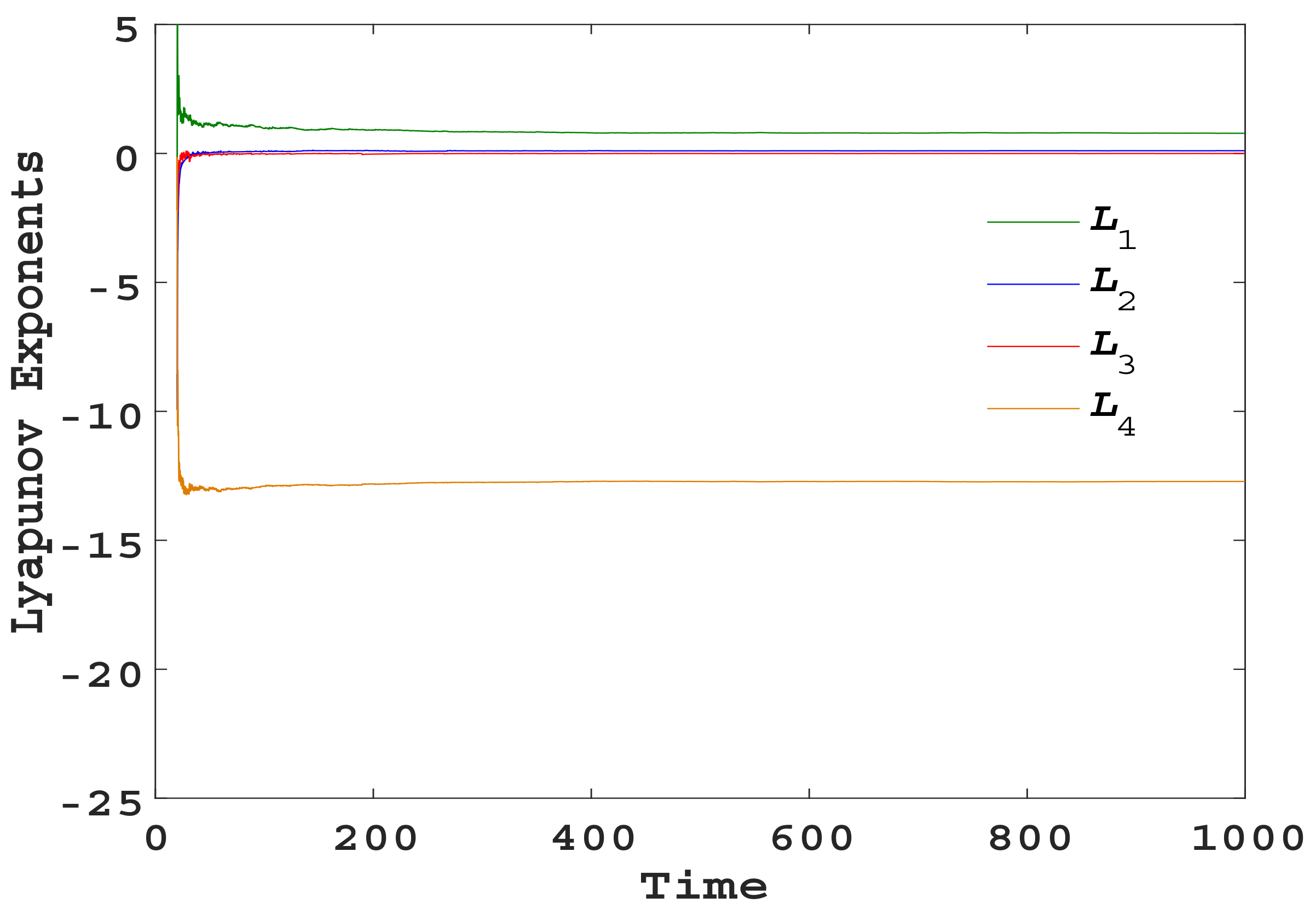
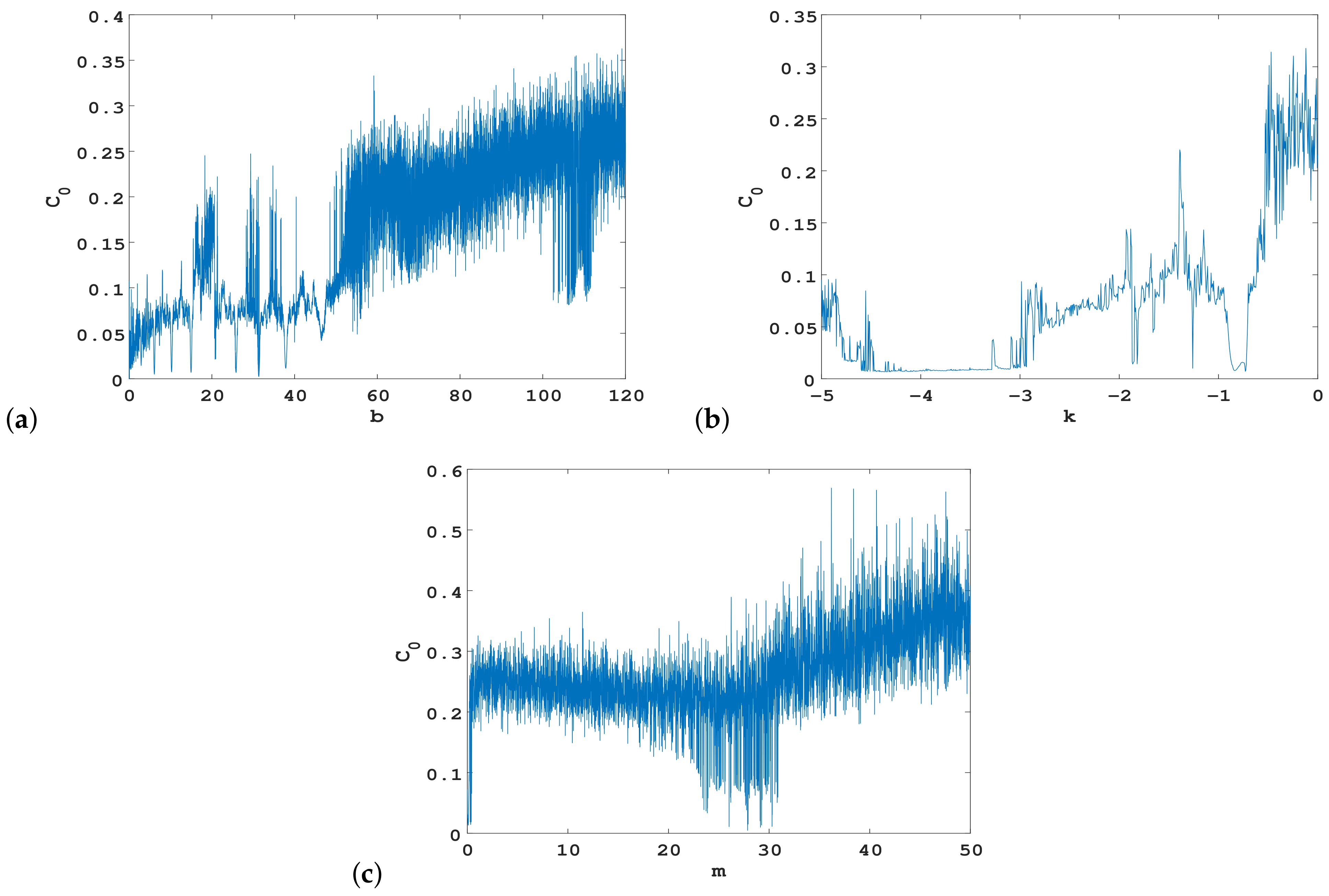
3.1. Lyapunov Exponents, Bifurcation Diagram, and $C_0$ Complexity Analysis

To explore the influence of b on the dynamics of the new 4D system, we fixed parameters $(a,c,k,m)=(10,2.7,-0.2,1)$, and varied b in the interval $[0,120]$. As we know, the main dynamical properties of system (2) can be analyzed by its Lyapunov exponent spectrum and bifurcation diagram. We took the initial values as $(x_0,y_0,z_0,w_0)=(1.67610,-0.37856,3.69140,1.45851).$ Figure 5a,b show the changes of four Lyapunov exponents with the increase of b, and Figure 5c gives the corresponding bifurcation diagram with respect to b. It can be observed that the Lyapunov exponent spectrum well coincides with the bifurcation diagram. It can be clearly seen from Figure 5 that system (2) indeed produces hyperchaotic attractors with two positive Lyapunov exponents for a wide range of $b.$ Three-dimensional projections of attractors for some typical values of b, are shown in Figure 6, and the corresponding Lyapunov exponents and fractal dimensions are tabulated in

Table 1. Lyapunov exponents and Kaplan–Yorke dimension of system (2) with $a=10,c=2.7$, $k=-0.2$, and $m=1.$

b	${\mathit{L}}_1$	${\mathit{L}}_2$	${\mathit{L}}_3$	${\mathit{L}}_4$	${\mathit{D}}_{\mathit{KY}}$	Dynamics
10	0	−0.0377	−0.4173	−11.6842	1.0	Periodic
20	0.0483	0	−0.2258	−11.9110	2.24	Chaos
38	0	−0.0227	−0.0243	−12.0242	1.0	Periodic
42	0	0	−0.1340	−11.9278	2.0	Quasi-periodic
50	0.0182	0	−0.2922	−11.7656	2.06	Chaos
120	0.9302	0.0850	0	−12.8638	3.08	Hyperchaos

, from which the intricate topological structure and abundant hyperchaotic dynamic properties of system (2) can be seen.

The $C_0$ complexity analysis relating to different parameters in new system (2) was also investigated, as shown in Figure 7. Compared with Figure 5, we can see that when the system is in a periodic state, the value of the $C_0$ complexity is small, whereas when the system is in a chaotic state or hyperchaotic state, the value of $C_0$ fluctuates between 0.1 and 0.4, which is significantly larger than that of the periodic state. Therefore, there is a positive correlation between the $C_0$ complexity measure and Lyapunov exponents, which can reflect the dynamic characteristics and complexity of the system.

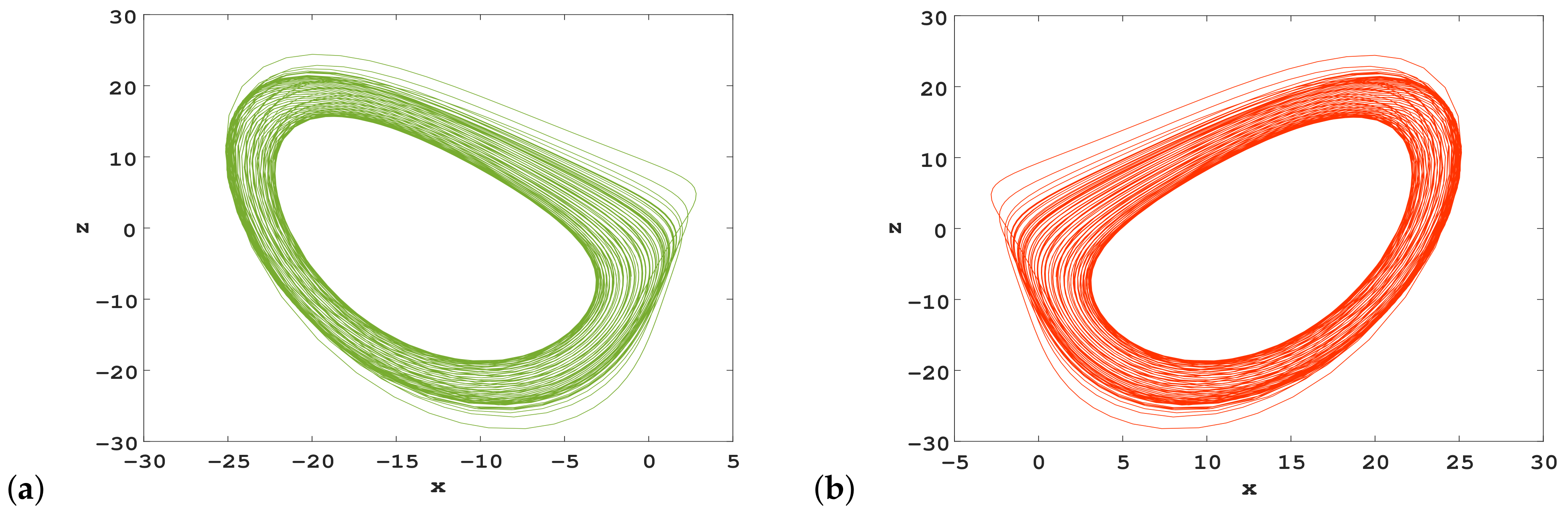
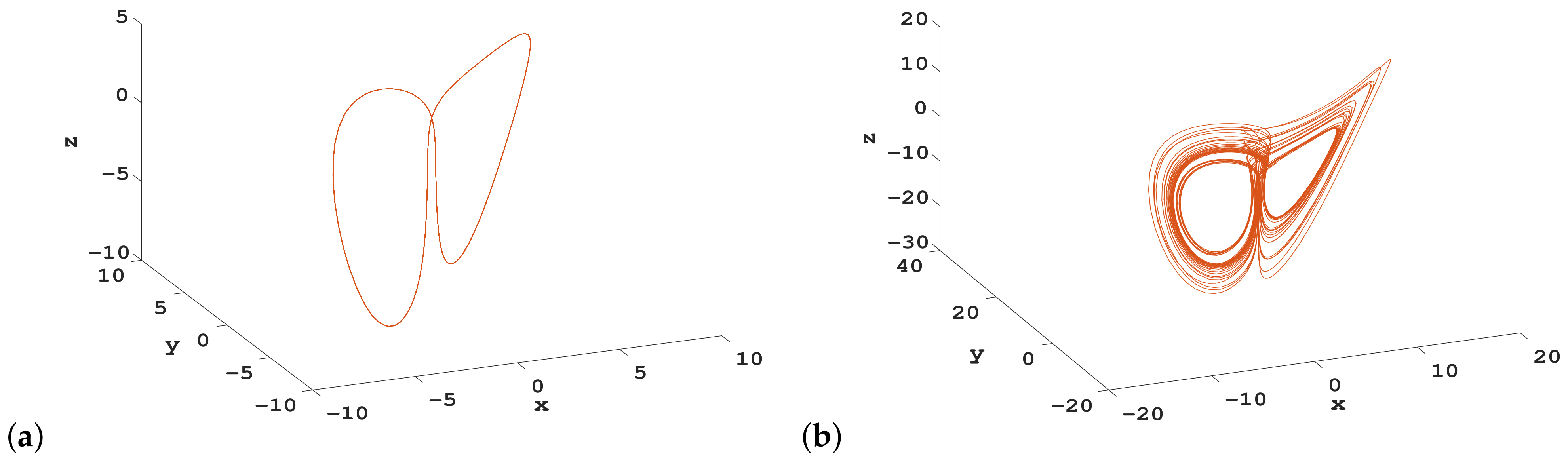
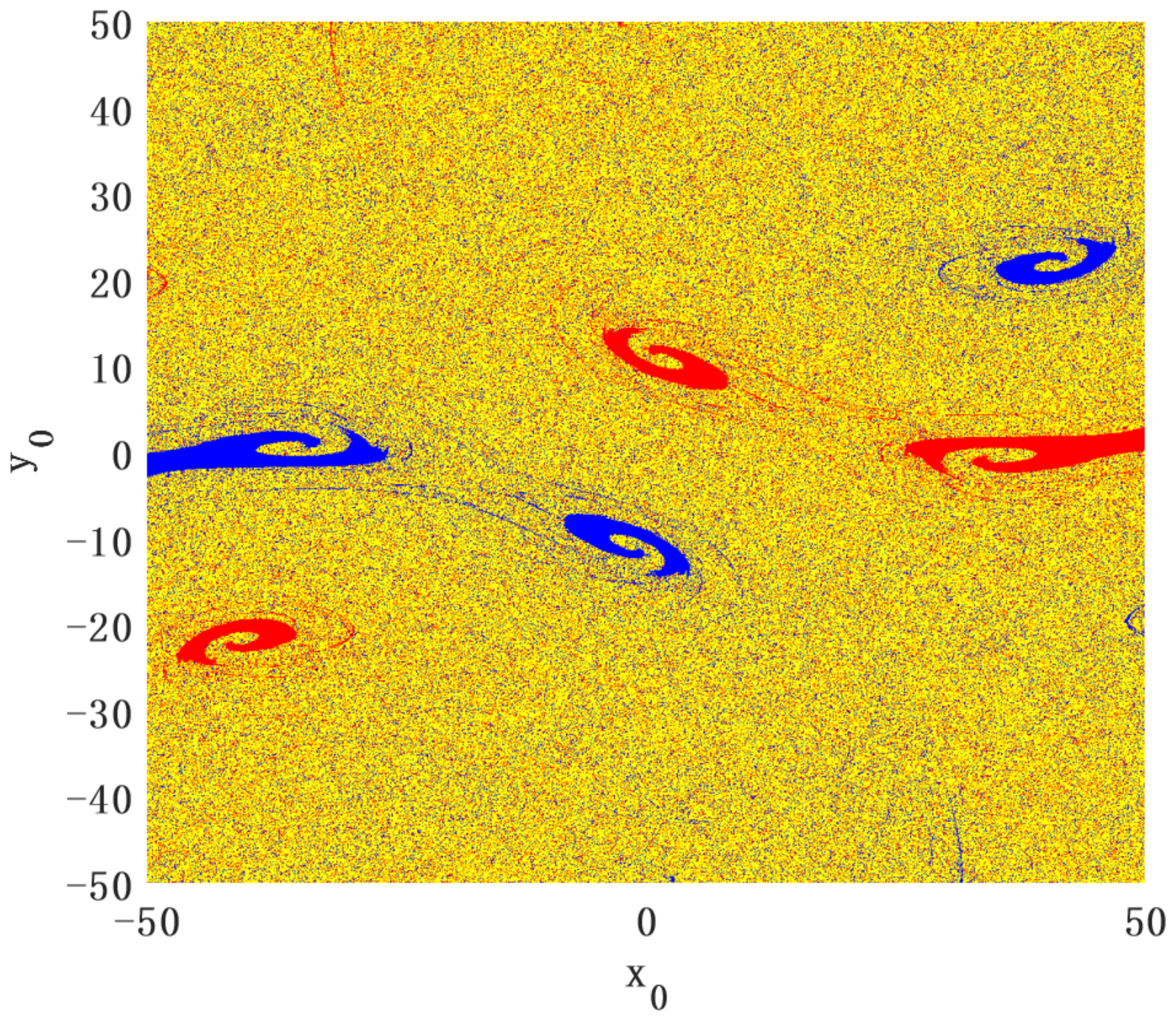
3.2. Coexisting Attractors

As discussed above, system (2) shows many complex dynamics, such as hyperchaos, chaos, and quasi-periodic and periodic motions. Several coexisting attractors of system (2) will be present under some appropriate parameters, indicating that hidden multistability emerges. A system with coexisting attractors is very sensitive to the initial values, noise, and system parameters. Importantly, under sudden disturbance, the state of the system can easily change and switch from an ideal state to another state that may be undesirable. However, multistability can make systems more flexible without adjusting parameters, and can be used with the correct control strategy to induce switching between various coexistence states. The coexisting attractors of system (2) satisfying different initial values may exhibit various dynamical behaviors.

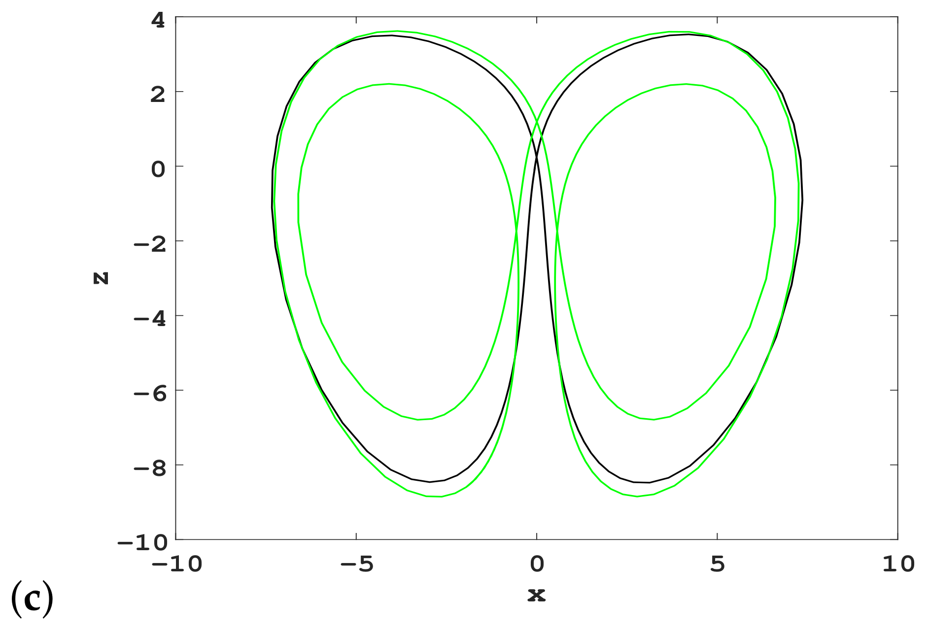
3.2.1. Coexistence of Chaotic and Periodic Attractors

When we take the parameters $(a,b,c,k,m)=(10,12,2.7,-0.2,1),$ the dynamic behavior of system (2) may change greatly in the long run:

(a) For initial values $(x_0,y_0,z_0,w_0)=(1,1,1,1),$ the Lyapunov exponents can be calculated as $L_1=0.037,L_2=0,L_3=-0.2098,$ and $L_4=-11.9386,$ and the fractal dimension of the system is estimated to be $2.1765$. A hidden chaotic attractor with no equilibrium point can be revealed, whose 2D phase portrait is shown in Figure 8a;

(b) For initial values $(x_0,y_0,z_0,w_0)=(-0.9,-1,-8,-1.7),$ the trajectory of the system converges to a stable periodic orbit, as shown in Figure 8b. The Lyapunov exponents of the system are found to be $L_1=0,L_2=-0.0144,L_3=-0.6047,$ and $L_4=-11.5121,$ and the Kaplan–Yorke dimension is $1.0$.

Hence, for parameters $(a,b,c,k,m)=(10,12,2.7,-0.2,1)$, system (2) has intricate dynamics with coexisting chaotic and periodic attractors, as shown in Figure 8c.

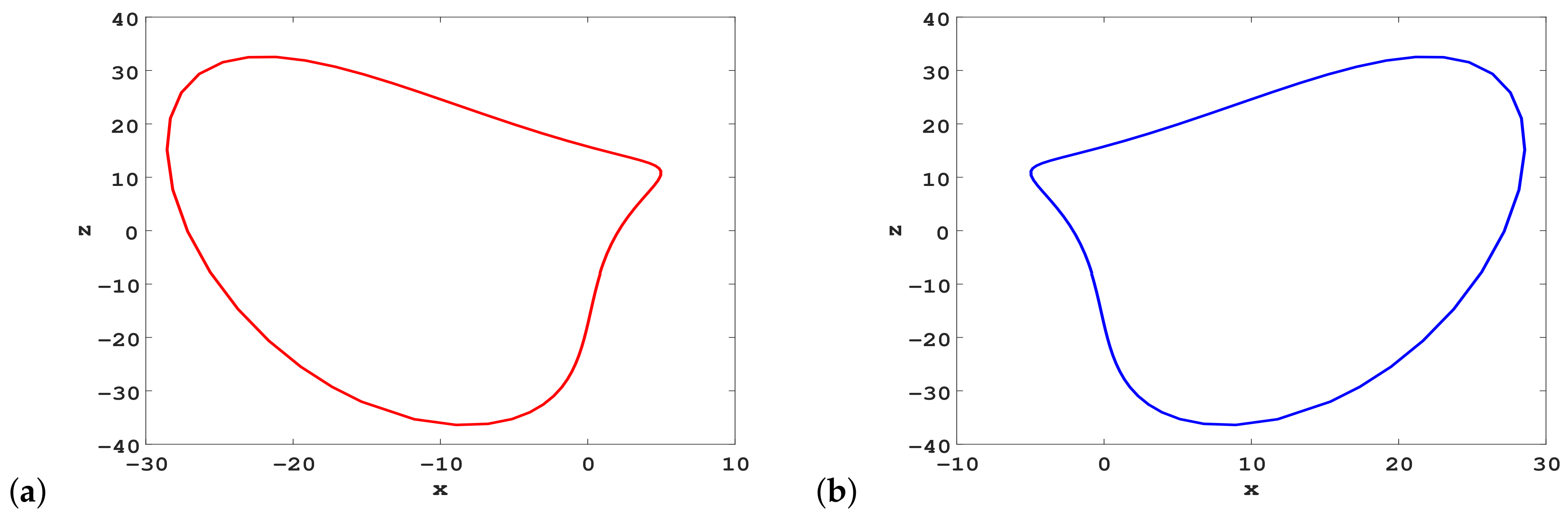
3.2.2. Coexistence of Quasi-Periodic and Periodic Attractors

When we take the parameters $(a,b,c,k,m)=(10,24,2.7,-0.2,1)$ and change the initial values, the dynamic behavior of system (2) may produce different coexisting attractors:

(a) For initial values $(x_0,y_0,z_0,w_0)=(0.885798,0.890960,-7.338199,1.357681),$ the Lyapunov exponents of system (2) are calculated as $L_1=0,L_2=0,L_3=-0.7809,$ and $L_4=-11.3183,$ and the Kaplan–Yorke dimension of the system can be estimated as $2.0$. Because there are two zeros and two negative Lyapunov exponents, system (2) experiences dynamical motion, which is called a quasi-periodic attractor, as depicted in Figure 9a;

(b) For initial values $(x_0,y_0,z_0,w_0)=(-0.8,-0.8,-6.8,-1.8),$ the trajectory of the system converges to a periodic orbit, as shown in Figure 9b. The Lyapunov exponents are found to be $L_1=0,L_2=-0.004,L_3=-0.5976,$ and $L_4=-11.4953,$ and the Kaplan–Yorke dimension is $1.0$.

Hence, for parameters $(a,b,c,k,m)=(10,24,2.7,-0.2,1)$, quasi-periodic and periodic attractors of system (2) coexist, as shown in Figure 9c.

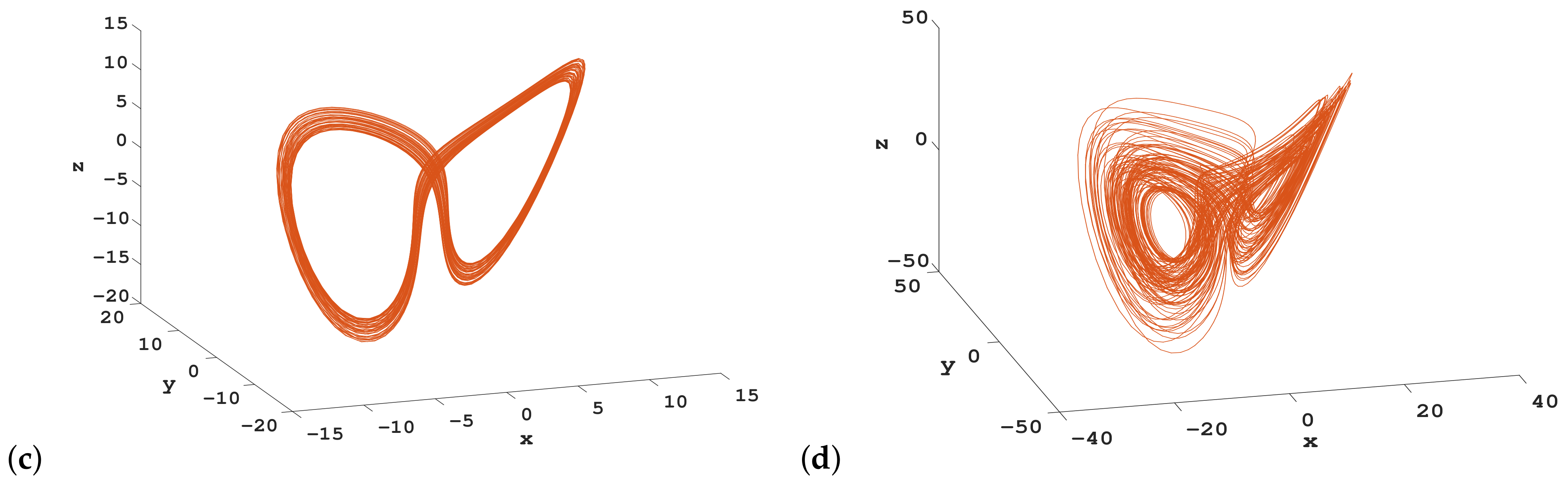
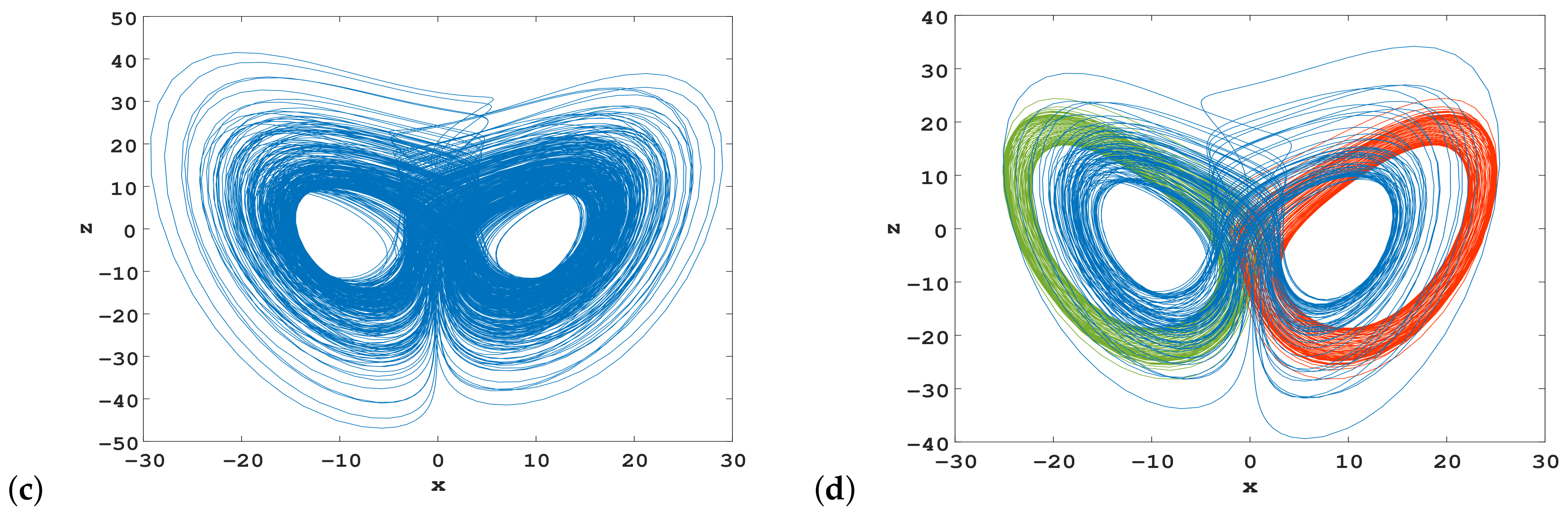
3.2.3. Coexistence of Chaotic and Quasi-Periodic Attractors

Let the parameters $(a,b,c,k,m)=(10,40,2.7,-0.2,2)$ and choose initial values $(1,2,5.2,1)$. The corresponding Lyapunov exponents are $L_1=0.0177,L_2=0,L_3=-0.1730,$ and $L_4=-11.9126,$ which means the attractor is chaotic. The corresponding fractal dimension is $2.0876$. The projection of this chaotic attractor onto the 2D phase space is presented in Figure 10a.

Choosing the same parameter values and taking initial values $(1,1,1,1)$, the four Lyapunov exponents are $L_1=0,L_2=0,L_3=-0.1686,$ and $L_4=-11.9045,$ which implies that system (2) has a quasi-periodic attractor, whose projection onto the 2D phase space is presented in Figure 10b.

Thus, for parameters $(a,b,c,k,m)=(10,40,2.7,-0.2,2)$, system (2) has complex dynamics with coexisting chaotic and quasi-periodic attractors, as illustrated in Figure 10c.

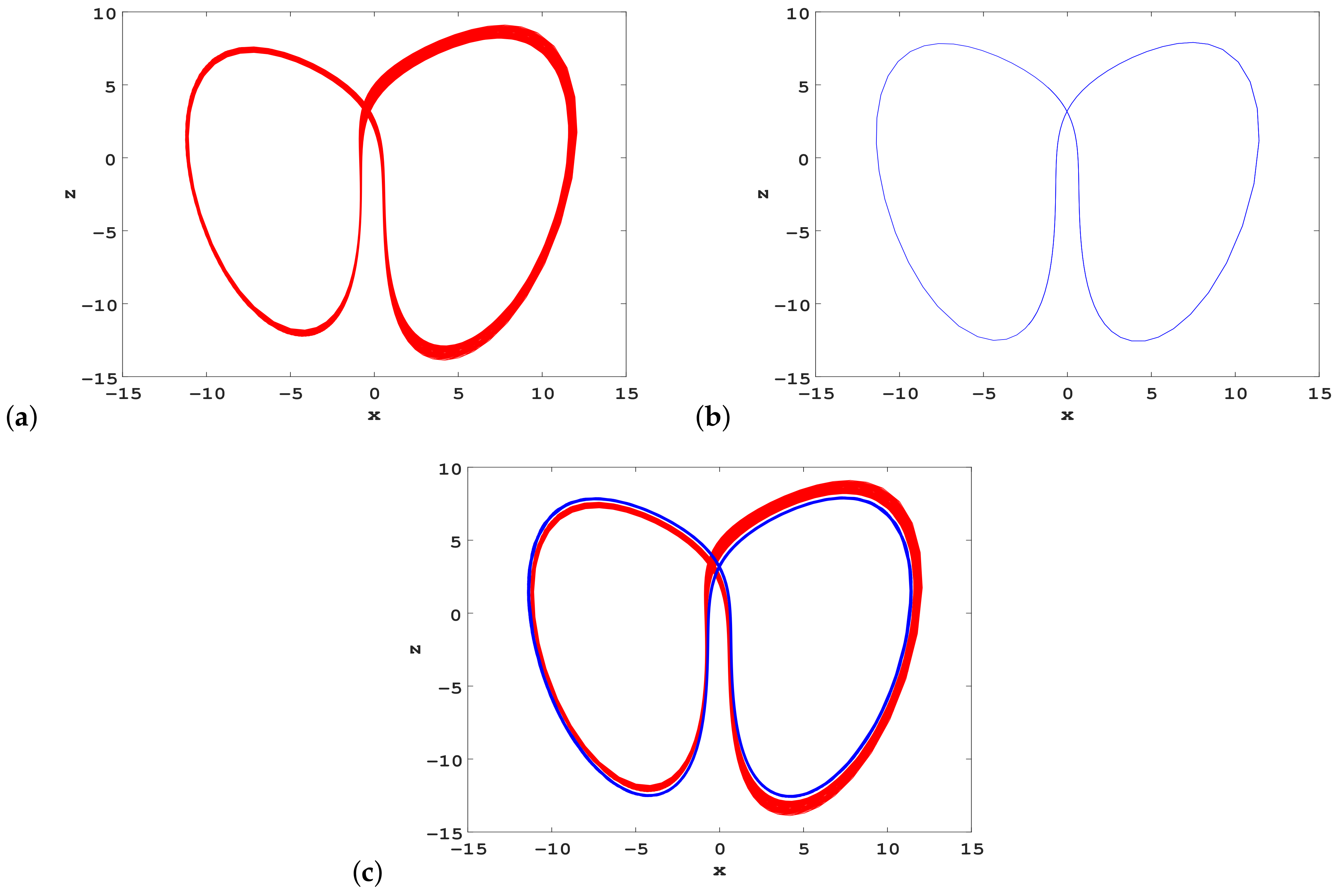
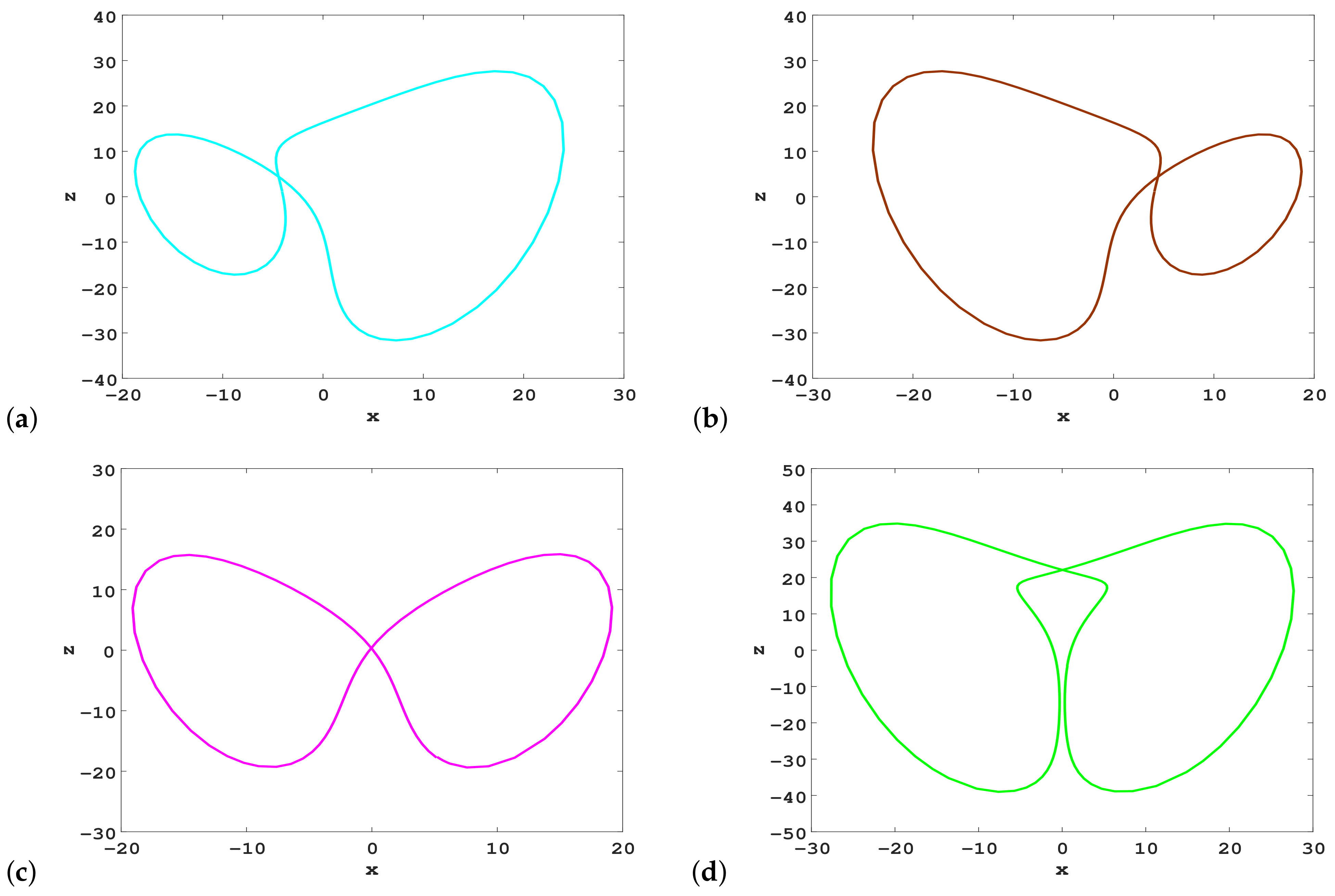
3.2.4. Coexistence of Hidden Periodic Attractors

Fixing the parameters $(a,b,c,k,m)=(10,10,2.7,-0.2,2)$ and choosing initial values $(-0.05,0.15,-0.04,-3.77)$, system (2) has a periodic attractor with projection onto the x–z plane, as presented in Figure 11a. The four Lyapunov exponents are $L_1=0,L_2=-0.0688,L_3=-0.0699,$ and $L_4=-12.0132$.

Choosing initial values $(-0.61,-0.38,-1.33,-0.79)$, one obtains the corresponding Lyapunov exponents $L_1=0,L_2=-0.0234,L_3=-0.0245,$ and $L_4=-12.1119$, which also implies a periodic attractor. The projection of the periodic attractor onto the 2D phase space is displayed in Figure 11b and has a different topology from the periodic attractor in Figure 11a.

Thus, we can conclude that two periodic attractors in system (2) coexist with parameters $(a,b,c,k,m)=(10,10,2.7,-0.2,2)$, as depicted in Figure 11c.

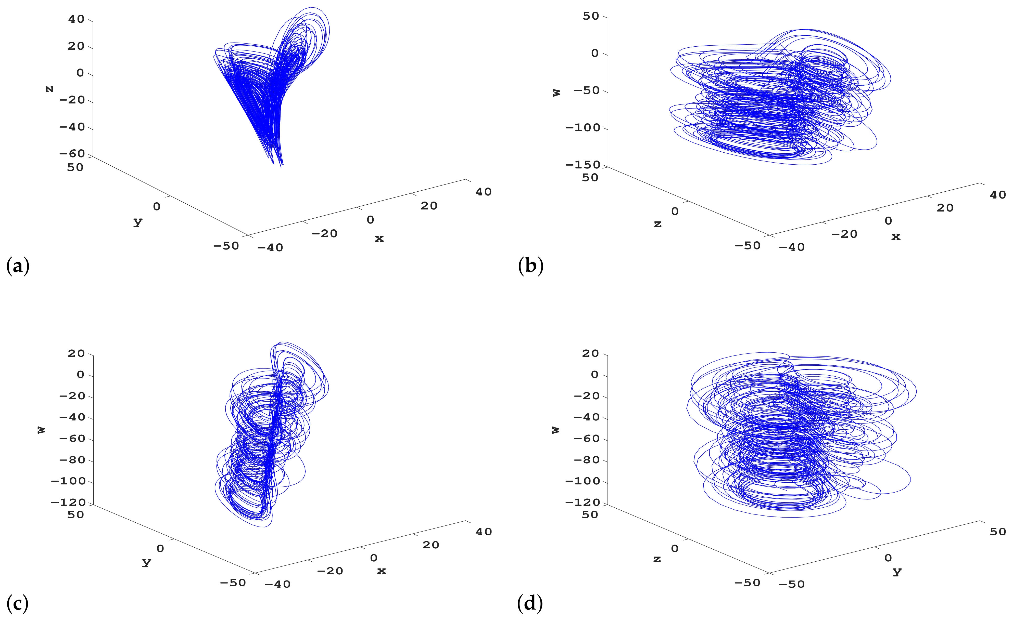
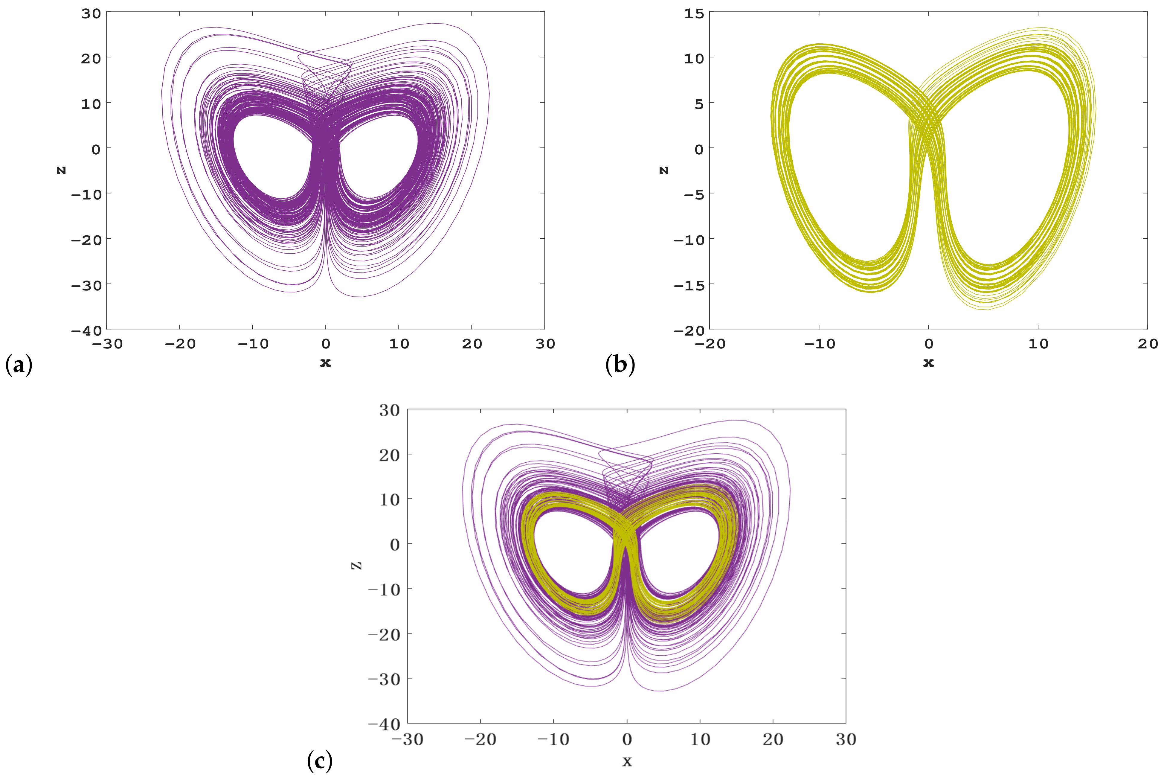
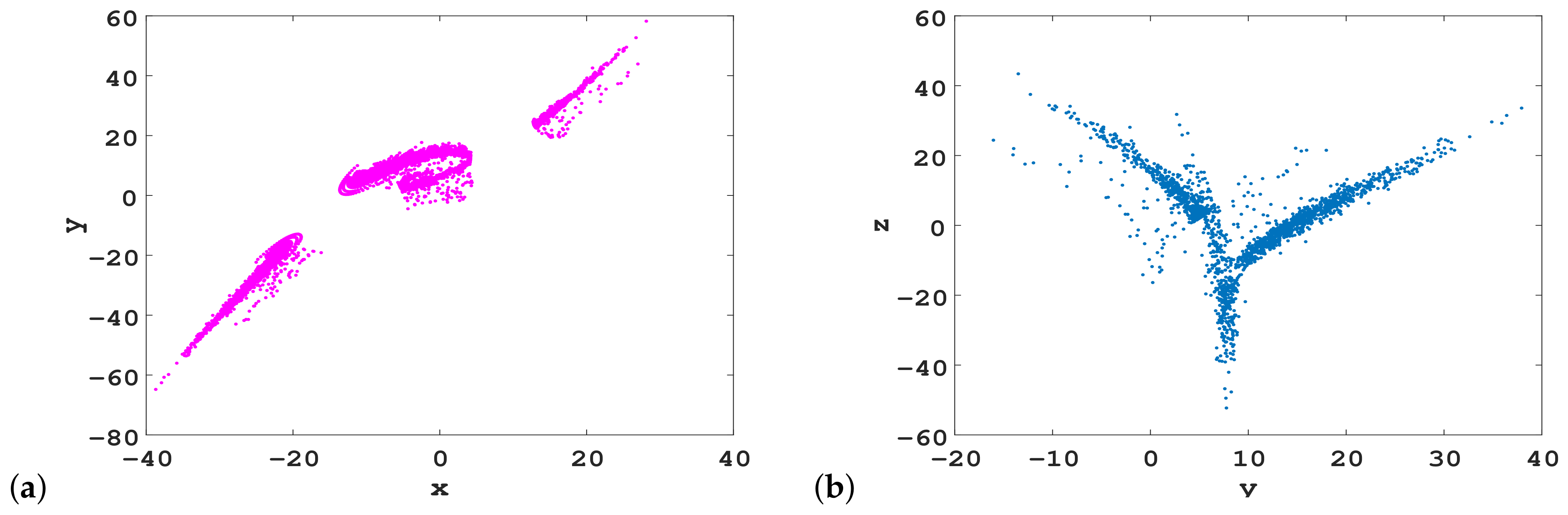
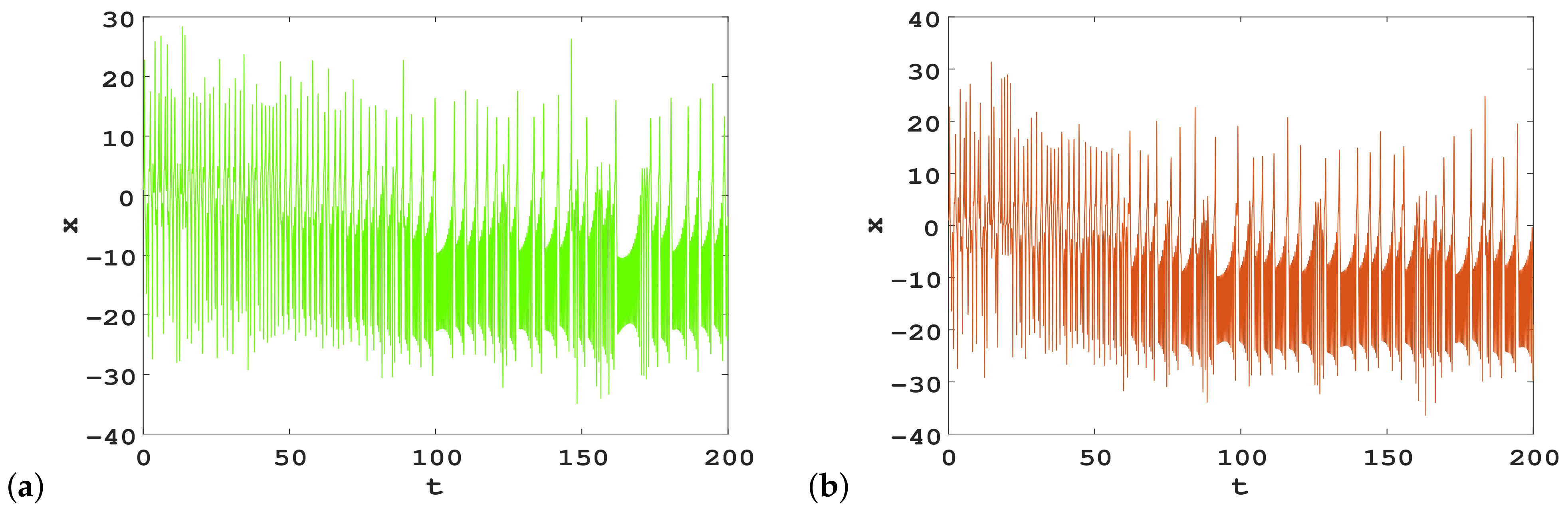
3.2.5. Coexistence of Hidden Hyperchaotic Attractors

Fixing the parameters $(a,b,c,k,m)=(10,70,2.7,-0.2,5)$ and taking the initial values $(1,-1,1,4)$, system (2) has an asymmetrical hidden hyperchaotic attractor with projection onto the x–z plane, as shown in Figure 12a. The four Lyapunov exponents are $L_1=0.2069,L_2=0.1033,L_3=-0.1665,$ and $L_4=-12.0257$. The corresponding fractal dimension is $3.0119$.

Based on the symmetry about the z-axis of system (2), if we choose initial values $(-1,1,1,-4)$, the other asymmetrical hidden hyperchaotic attractor can be obtained, whose 2D phase portrait is shown in Figure 12b. The two attractors have the same Lyapunov exponents and fractal dimension.

Choosing the same parameters and taking initial values $(1,1,1,1)$, the four Lyapunov exponents are $L_1=0.4159,L_2=0.2456,L_3=0,$ and $L_4=-12.6681$, and the Kaplan–Yorke dimension is $3.0521$. A symmetrical hidden hyperchaotic attractor can be found, whose projection onto the 2D phase space is presented in Figure 12c.

Through the above analysis, we can observe that system (2) simultaneously has three coexisting hidden hyperchaotic attractors under parameters $(a,b,c,k,m)=(10,70,2.7,-0.2,5)$, as shown in Figure 12d. The basins of attraction of three coexisting hidden hyperchaotic attractors can also be calculated, as shown in Figure 13, where the yellow area denotes the basin of attraction of a symmetrical hyperchaotic attractor, while the red and blue areas represent the basin of attraction of an asymmetrical hyperchaotic attractor presented in Figure 12a,b, respectively. Riddled basins can be observed in Figure 13, which means that the dynamical behaviors of the proposed 4D system are extremely sensitive to the initial values.

4. Analysis of Unstable Cycles for New 4D Hyperchaotic System via Variational Approach

In this section, we employ the variational calculation approach for the unstable periodic orbit search and establish an appropriate symbolic encoding for the found cycles. We also analyze the continuous deformations of cycles by the homotopy evolution method, which shows applicable flexibility under different circumstances. We aim to accurately find the encircling way of the orbit in the new 4D hyperchaotic system and develop an effective way to classify periodic orbits. Several short periodic orbits in system (2) are located, and the evolution law of the period of cycle alteration with parameters is discussed, which indicates that the proposed method is effective at analyzing unstable periodic orbits.

4.1. Variational Method for Calculations

Strange attractors in hyperchaotic systems are densely covered by countless unstable periodic orbits. Therefore, extracting unstable cycles usually has an important influence on understanding their properties. Many numerical methods are employed to extract the periodic orbits of various systems [45]. We utilized the variational method in this paper, which has shown its reliability and efficiency [46]. The basic physical idea is to make an initial loop guess about the shape of the periodic orbit, and then gradually evolve it into a real periodic orbit. Initialization is important in the variational calculations, as it determines whether the calculated periodic orbit is the one of interest, and it can be implemented by various means [47].

Using the variational method to locate periodic orbits, a discretization equation,

$$\left(\begin{array}{cc}\stackrel{\wedge }{A}& -\stackrel{\wedge }{v}\\ \stackrel{\wedge }{a}& 0\end{array}\right)\left(\genfrac{}{}{0pt}{}{\delta \stackrel{\sim }{x}}{\delta \lambda }\right)=\delta \tau \left(\genfrac{}{}{0pt}{}{\lambda \stackrel{\wedge }{v}-\stackrel{\wedge }{\stackrel{\sim }{v}}}{0}\right),$$

(4)

can be derived to solve for $\delta \stackrel{\sim }{x}$ and $\delta \lambda$, so as to achieve the location of the cycle and period [46]. Compared to other numerical methods, as a result of the use of a continuum of points, the variational method has the advantage of numerical stability. Furthermore, we do not need to choose a Poincaré section beforehand. The variational method can be used to calculate the stable or unstable periodic orbits of various systems [48,49,50]. In addition, the continuous deformation of cycles with the variation of parameters can be studied based on the variational method, and the bifurcation phenomenon can be observed by analyzing whether the number or stability of cycles has changed. Next, we use the variational method to extract the unstable cycles in system (2).

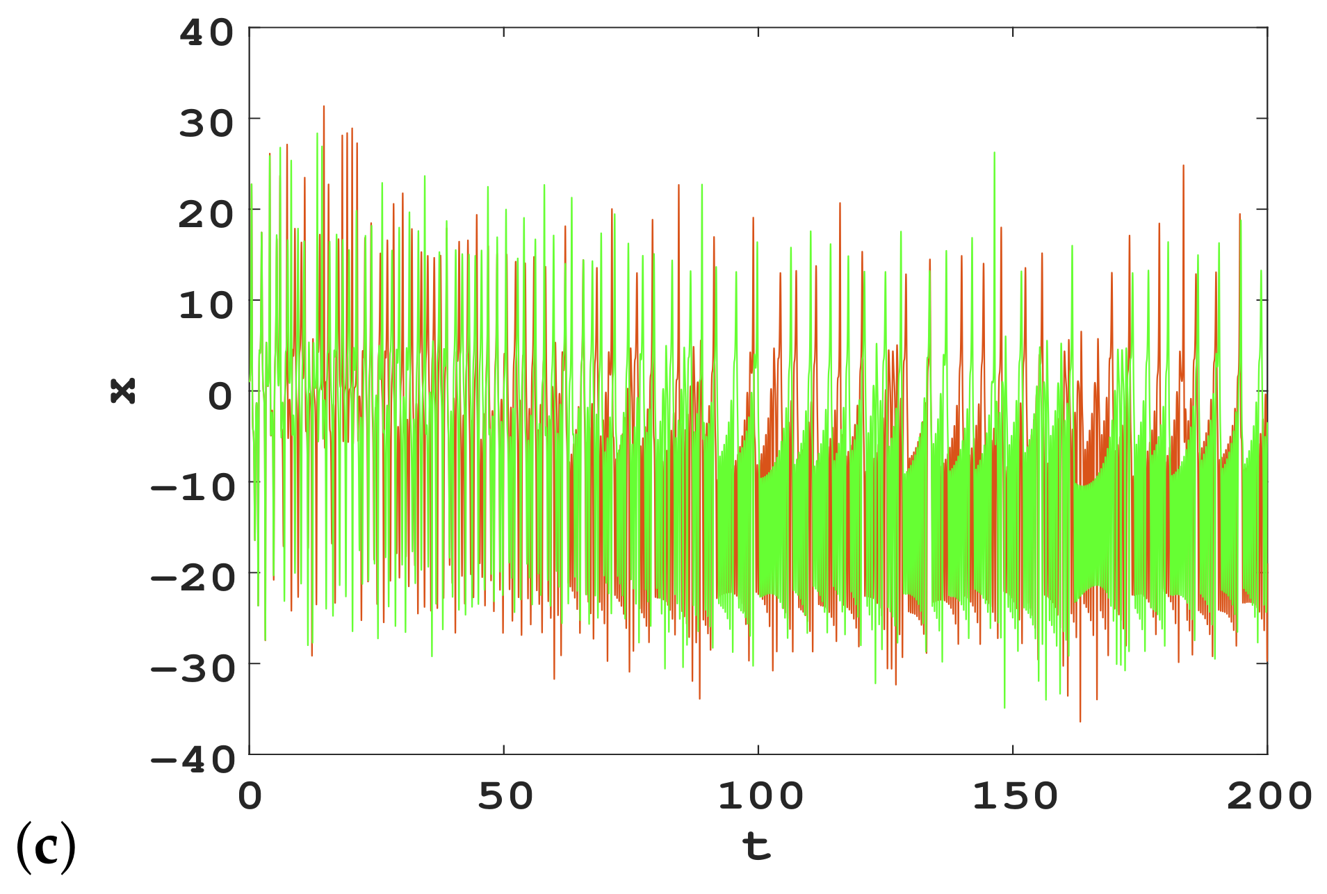
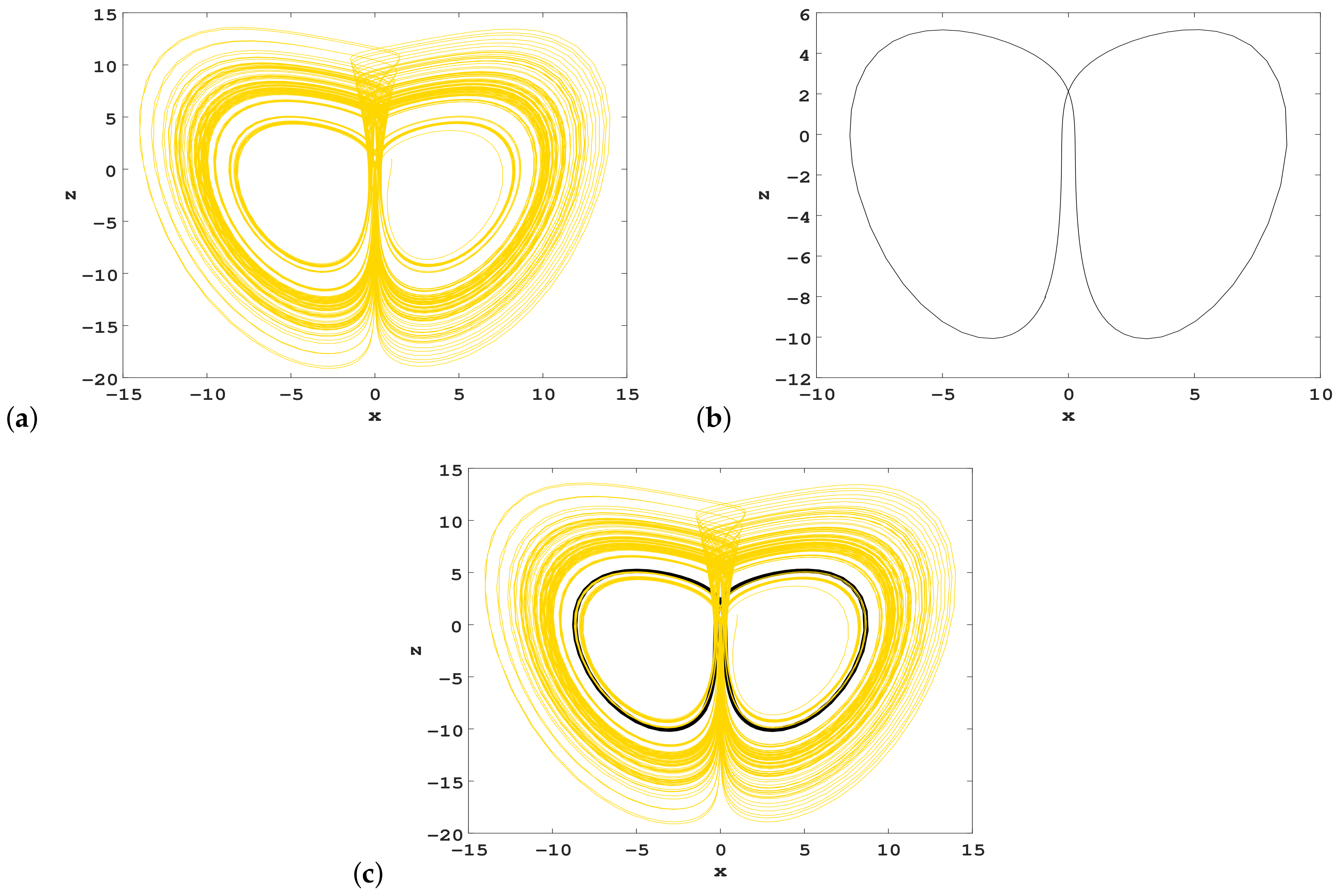
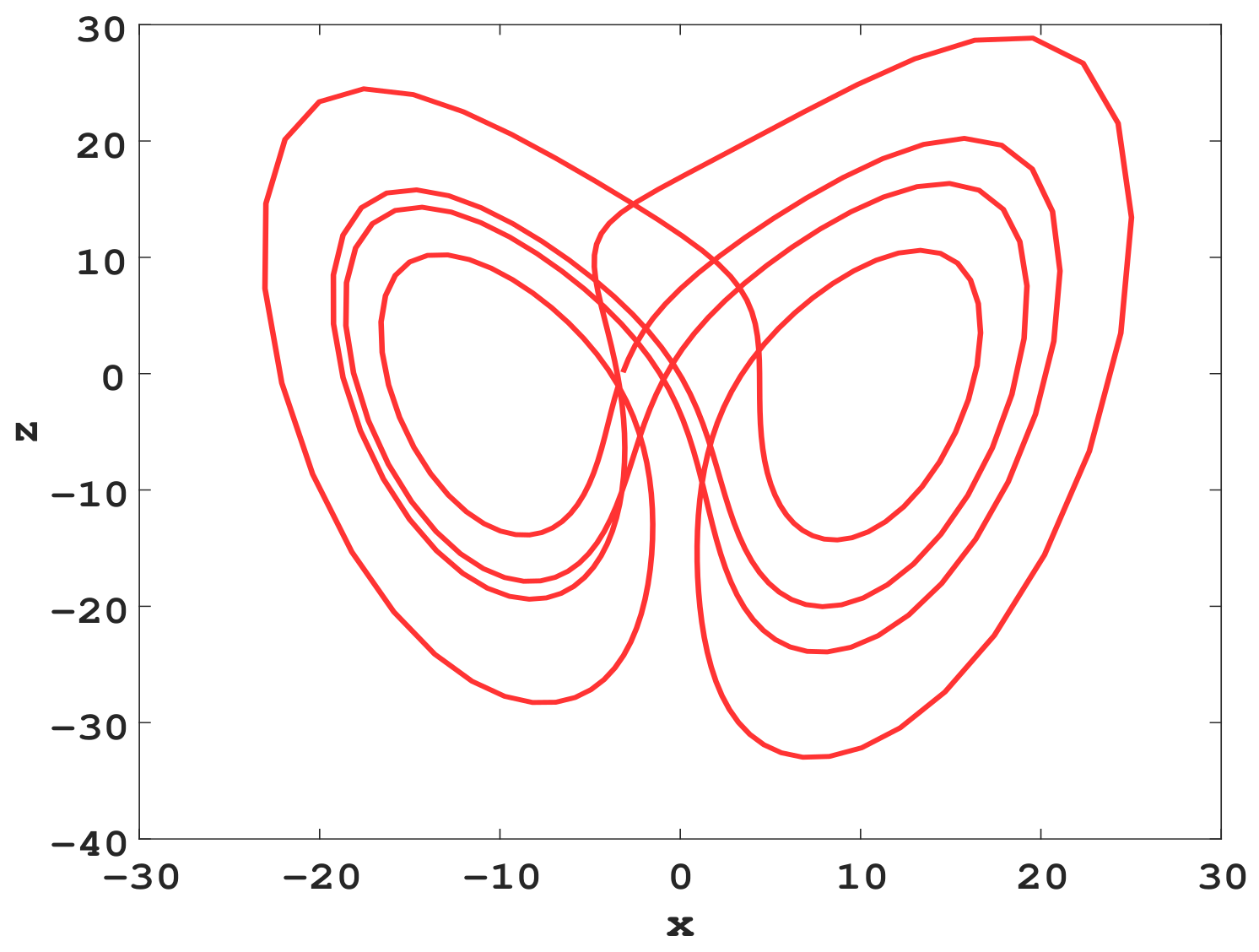
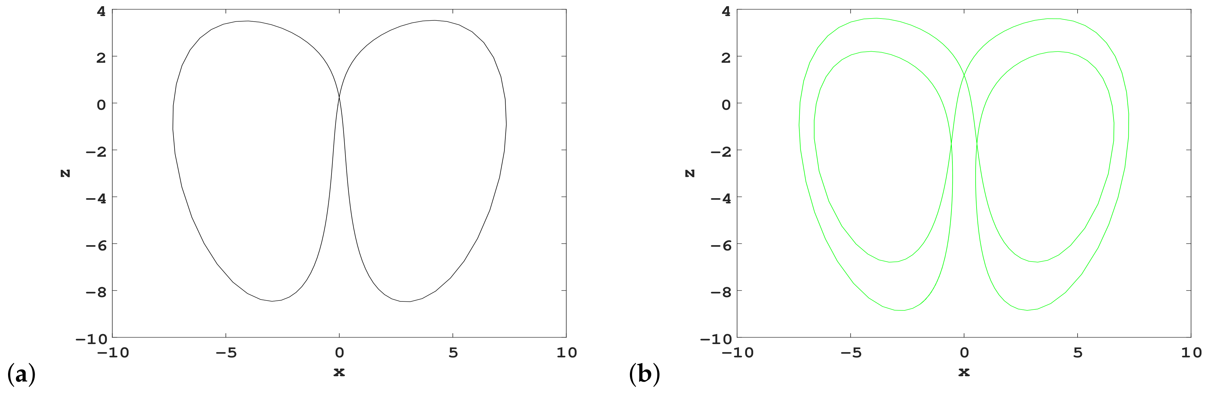
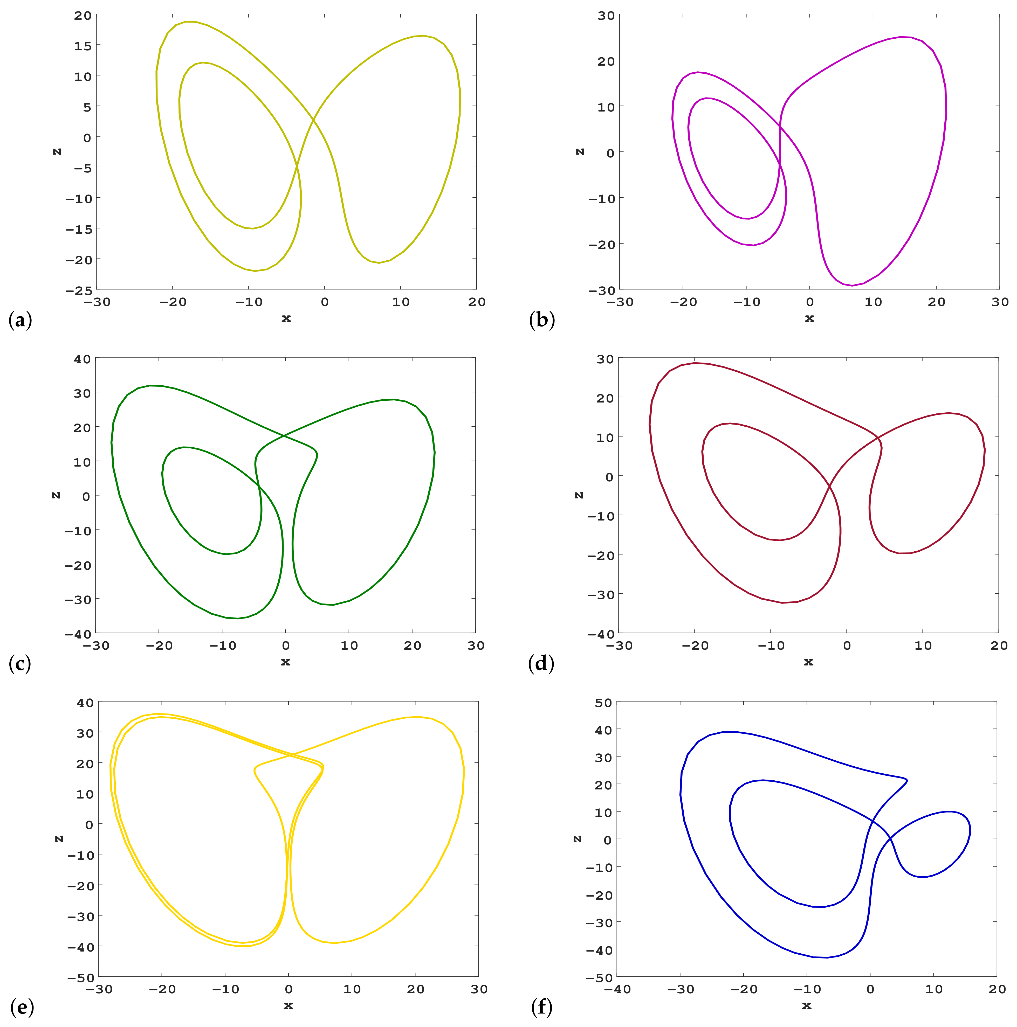
4.2. Extracting Unstable Cycles in a Hidden Hyperchaotic Attractor

We calculated the unstable cycles embedded in a hidden hyperchaotic attractor with parameters $(a,b,c,k,m)=(10,100,2.7,-0.2,1)$ by the variational method. Symbols were used to encode them for cycles with different topological structures, so that all of the cycles could be located without duplication or being missing based on symbolic dynamics [51]. When utilizing the variational method for initialization, the segments of trajectories with similar shapes were obtained through numerical integration, and they were manually connected to close, so as to become a loop. By this approach, several cycles with different complexity were found. Figure 14 shows two periodic orbits with the simplest topology; they have certain symmetry with each other and the shortest periods of the same size. Figure 15 shows four more intricate periodic orbits, which are composed of two building blocks of periodic orbits with different topologies.

Motivated by this observation, we marked the cycles in Figure 15a,b as 03 and 12, respectively; thus, the cycle in Figure 14a is cycle 2, and that in Figure 14b is cycle 3. We did not find cycle 0 or 1, which means that they were pruned. With the help of four basic orbital segments, longer periodic orbits can also be encoded and calculated. Figure 16 shows six cycles with topological length 3. In total, we found 18 periodic orbits within topological length 3, which are listed in

Table 2. Eighteen unstable periodic orbits embedded in the hidden hyperchaotic attractor of system (2) for $(a,b,c,k,m)=(10,100,2.7,-0.2,1)$; listed are the topological length, itinerary p, period $T_p$, and four coordinates of a point on the cycle.

Length	p	${\mathit{T}}_{\mathit{p}}$	x	y	z	w
1	2	0.858233	0.851259	3.599482	−8.032931	−39.656931
	3	0.858233	−0.851259	−3.599482	−8.032931	39.656931
2	03	1.362034	−4.076805	−1.813737	1.109695	−14.135359
	12	1.362034	4.076805	1.813737	1.109695	14.135359
	01	1.194275	5.206540	7.525051	−17.639962	1.385740
	23	1.830597	0.626331	−0.321247	−4.302274	1.490707
3	001	1.732553	−5.282481	3.245260	0.268165	−34.418329
	011	1.732553	5.282481	−3.245260	0.268165	34.418329
	003	1.821191	−4.653735	2.777113	−2.962048	−38.837657
	112	1.821191	4.653735	−2.777113	−2.962048	38.837657
	132	2.211630	11.320228	14.639216	−16.413004	25.186818
	023	2.211630	−11.320228	−14.639216	−16.413004	−25.186818
	021	1.968277	−6.298304	3.295041	5.572765	−20.401797
	013	1.968277	6.298304	−3.295041	5.572765	20.401797
	223	2.766255	1.453074	−0.422130	2.547336	1.463103
	233	2.766255	−1.453074	0.422130	2.547336	−1.463103
	012	2.207939	4.137109	5.676602	−5.643553	−9.306008
	031	2.207939	−4.137109	−5.676602	−5.643553	9.306008

. It is worth noting that the symmetry of system (2) can also be seen from Table 2. The two cycles of commutative symbols 0 and 1, or 2 and 3, are conjugate to each other, and they have the same periods.

According to the above encoding rules, other complex long periodic orbits can also be calculated as follows. We generated the initial loop guess based on the symbol sequence corresponding to the cycle, and employed the variational method to verify whether the cycle existed. Figure 17 shows an unstable cycle with a topological length of 8, with corresponding symbol encoding 02130101. The successful search of such complex periodic orbits also shows the effectiveness of our encoding method in calculating various periodic orbits embedded in a hidden hyperchaotic attractor.

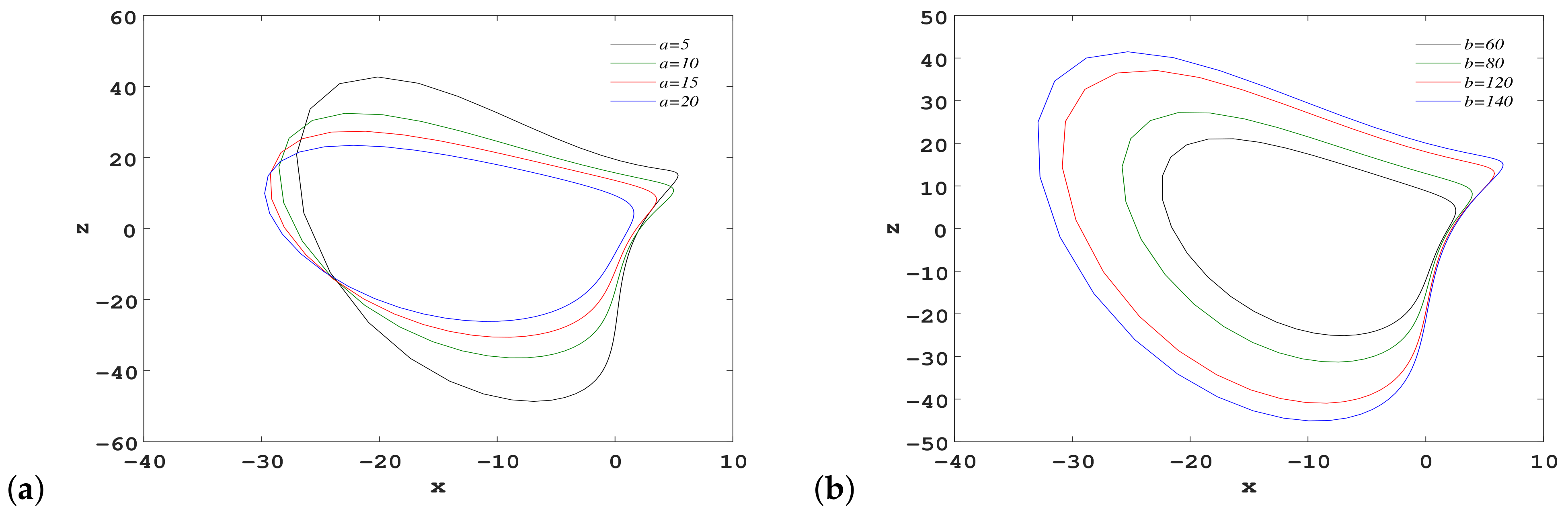
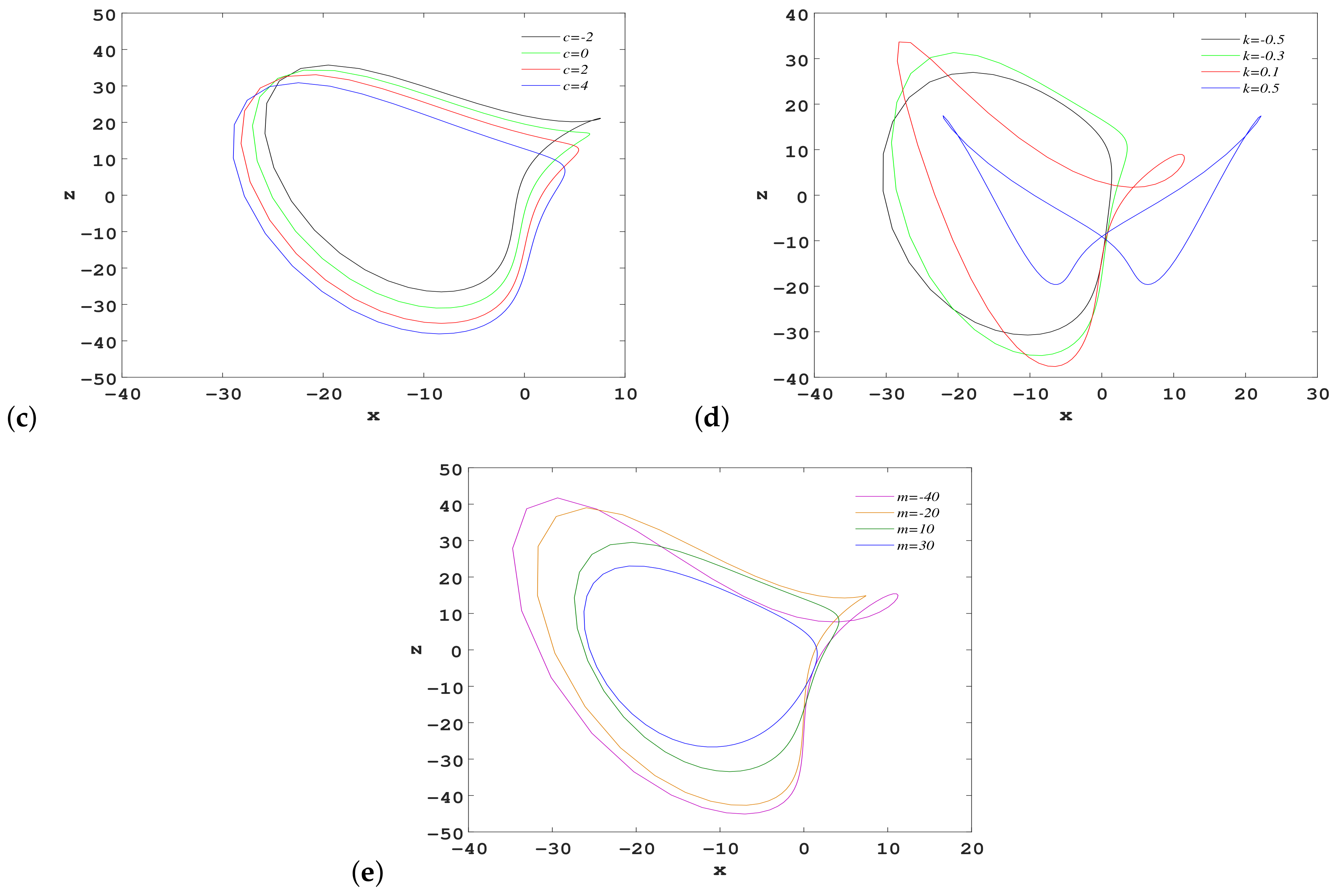
4.3. Homotopy Evolution of Cycle Variation with Different Parameters

With the change of different parameters, the number of periodic orbits and their stability can undergo changes, which means that bifurcations may occur [52]; the variational approach is convenient to study various bifurcation behaviors. We studied the evolution of unstable cycles of system (2) when parameters were altered, and the homotopy evolution method could be conveniently used for the initialization [53]. For a dynamical system, when the parameters alter little, most short cycles experience slight deformation unless bifurcation occurs. Therefore, the periodic orbits previously calculated with given parameters could be taken as the initial loop guess for the next calculations. Initializing in this way, the calculations of cycles were very efficient.

First, the bifurcations of periodic orbits were investigated by varying a while fixing $b=100,$$c=2.7,k=-0.2,$ and $m=1.$ We used the previously calculated cycle 2 as the initial loop guess to calculate cycle 2 for the next a value. Figure 18a illustrates the homotopy evolution cases. We found that when $a<5$ or $a>20$, the calculation of cycle 2 by the variational method was no longer convergent. Thus, we can conclude that the system experiences periodic orbit bifurcations at $a=5$ and $a=20.$

Then, we studied the continuous deformation of cycle 2 with respect to the b value in the same way, fixing $a=10,$$c=2.7,k=-0.2,$ and $m=1$. Figure 18b shows the deformation of cycle 2 with the b value. We also found that the periodic orbit bifurcations occurred when $b=52.$ Similarly, we changed c, k, and m, respectively, and fixed the remaining parameters to study the continuous deformation of cycle 2; the homotopy evolution processes are shown in Figure 18c–e.

Table 3. Periods $T_p$ of cycle 2 for different parameters.

a	${\mathit{T}}_{\mathit{p}}$	b	${\mathit{T}}_{\mathit{p}}$	c	${\mathit{T}}_{\mathit{p}}$	k	${\mathit{T}}_{\mathit{p}}$	m	${\mathit{T}}_{\mathit{p}}$
5	1.082797	60	0.953492	−2	0.880703	−0.5	0.705715	−40	0.996271
10	0.858233	80	0.911549	0	0.873372	−0.3	0.821457	−20	0.968155
15	0.729400	120	0.811395	2	0.864607	0.1	0.964986	10	0.799075
20	0.610639	140	0.771540	4	0.833397	0.5	1.140899	30	0.611363

lists the periods $T_p$ of cycle 2 at different parameter values. By symmetry, it is obvious that cycle 3 has a similar deformation as the variation of parameters. The above discussion demonstrates that if we take a new set of parameters, new periodic orbits corresponding to the new period will appear, and some of the periodic orbits in Table 2 will no longer exist due to periodic orbit bifurcations.

Finally, we explored the evolution rule between the orbital period and different parameters. From Table 3, it can be concluded that the larger the parameters $a,b,c$, and m, the smaller the periods, and as k increases, the period becomes larger. We confirm that this conclusion is applicable to all of the other short cycles calculated in system (2).

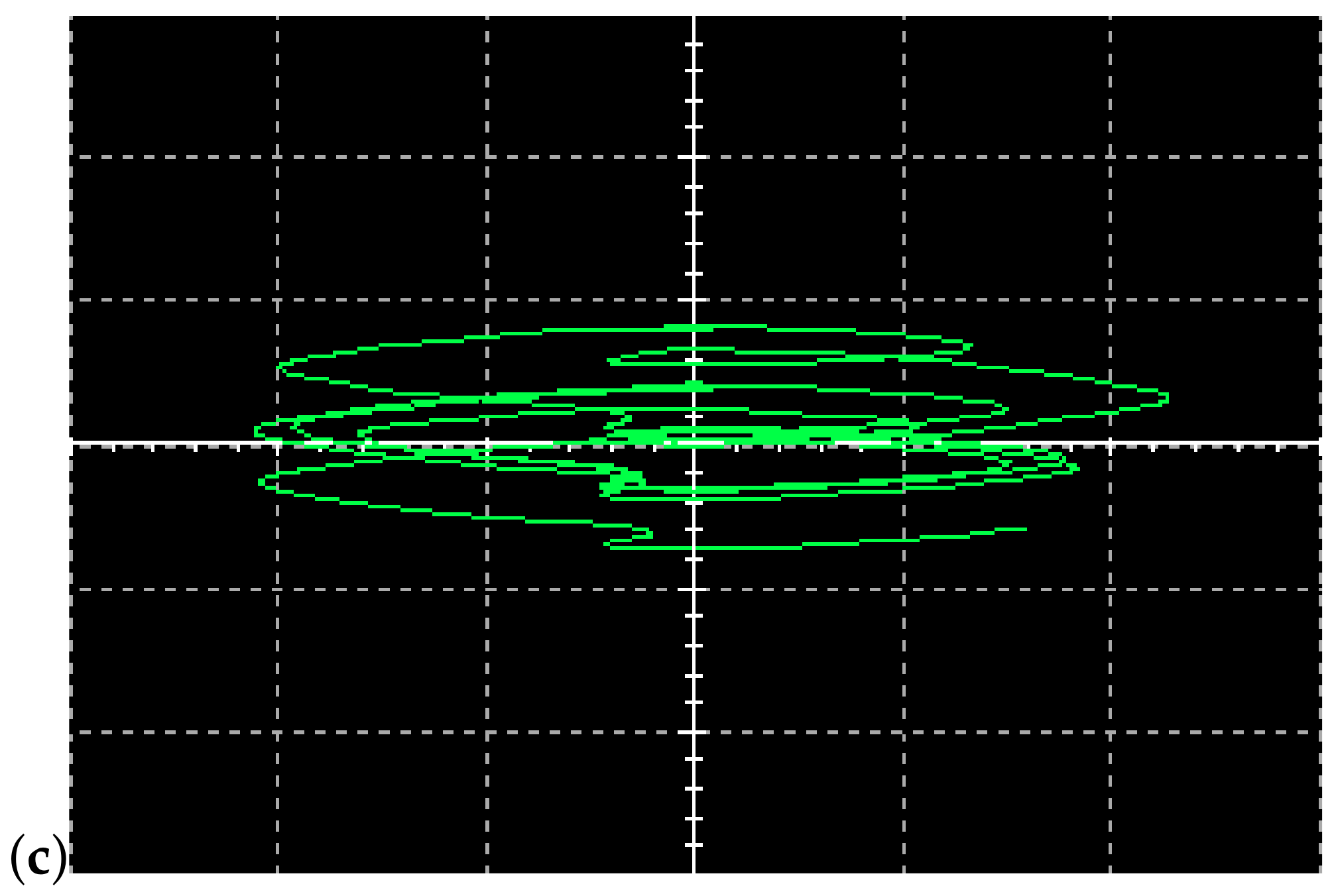
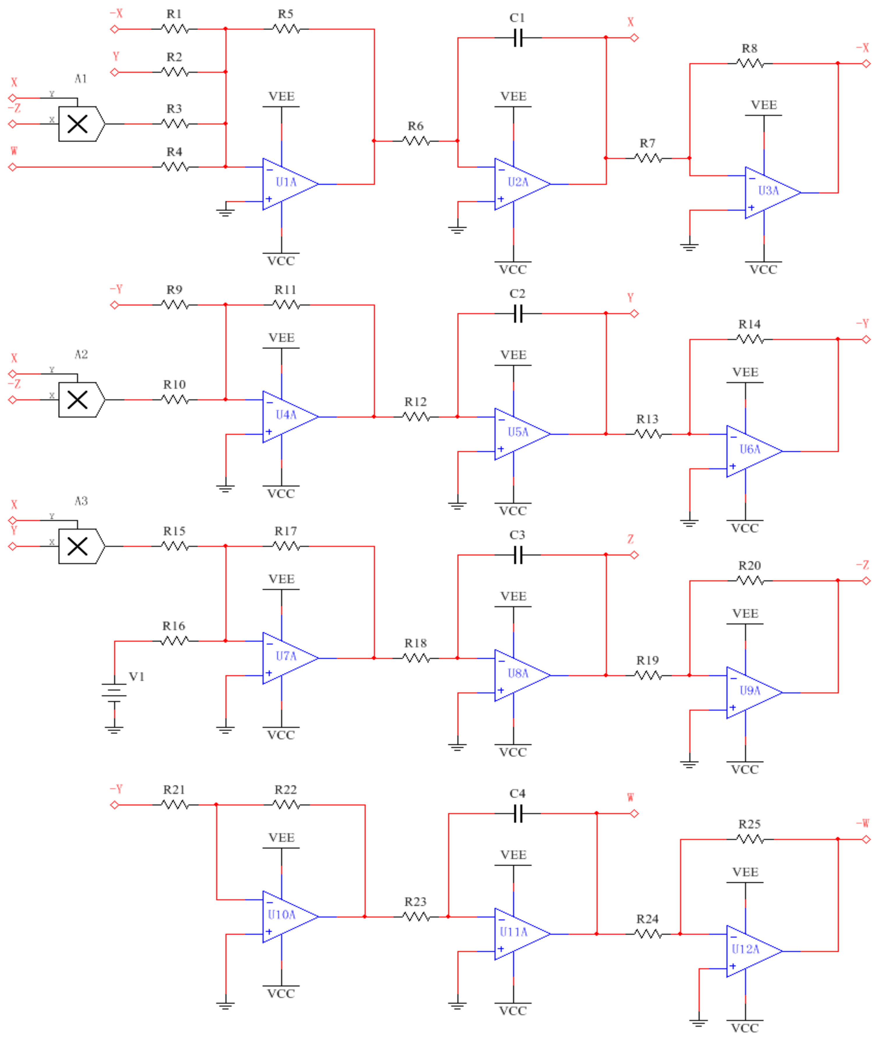
5. Circuit Design and Realization of New System

The circuit implementation can verify the feasibility and validity of a new chaotic system. The electronic synthesis of a novel antimonotic hyperjerk system was proposed based on an analog computing approach [54]. We employed Multisim simulation software to build a circuit. We selected four channels, corresponding to four state variables of the new system, to observe whether the results of the phase diagrams were consistent with the output of the actual circuit. The main task was to design and implement the hyperchaotic system and verify the circuit that realized the coexistence of chaotic and periodic attractors. Since the state variables of system (2) were beyond the dynamic range of the device, a proportional transformation was required to set the amplitude scaling factor to 10, where $X=\frac{1}{10}x$, $Y=\frac{1}{10}y$, $Z=\frac{1}{10}z$, and $W=\frac{1}{10}w$. Therefore, system (2) was rewritten as

$$\begin{array}{ccc}\hfill \stackrel{·}{X}& =& a(Y-X)+10kXZ+W\hfill \\ \hfill \stackrel{·}{Y}& =& -cY-10XZ\hfill \\ \hfill \stackrel{·}{Z}& =& -0.1b+10XY\hfill \\ \hfill \stackrel{·}{W}& =& -mY.\hfill \end{array}$$

(5)

We implemented a time-scale transformation of Equation (5), with the time scale factor set to ${\tau }_0=\frac{1}{R_0{C}_0}=1000$. A new time variable $\tau$ was used instead of t, and $t={\tau }_0\tau .$ As shown in Figure 1, a hyperchaotic attractor exists under the parameters $(a,b,c,k,m)=(10,100,2.7,-0.2,1)$. The proposed circuit design is depicted in Figure 19, in which three analog multipliers (the output gain was 0.1) were used to realize 3 nonlinear terms, 12 AD712AH operational amplifiers, 4 capacitors, and 25 resistances to realize the addition, integration, and inversion operations. The power supply voltage was $\pm 18$ V. Based on Kirchhoff’s law, the corresponding circuit equations can be derived as

$$\begin{array}{ccc}\hfill \stackrel{·}{X}& =& \frac{R_5}{R_2{R}_6{C}_1}Y-\frac{R_5}{R_1{R}_6{C}_1}X-\frac{R_5}{R_3{R}_6{C}_1}0.1XZ+\frac{R_5}{R_4{R}_6{C}_1}W\hfill \\ \hfill \stackrel{·}{Y}& =& -\frac{R_{11}}{R_9{R}_{12}{C}_2}Y-\frac{R_{11}}{R_{10}{R}_{12}{C}_2}0.1XZ\hfill \\ \hfill \stackrel{·}{Z}& =& \frac{R_{17}}{R_{16}{R}_{18}{C}_3}{V}_1+\frac{R_{17}}{R_{15}{R}_{18}{C}_3}0.1XY\hfill \\ \hfill \stackrel{·}{W}& =& -\frac{R_{22}}{R_{21}{R}_{23}{C}_4}Y.\hfill \end{array}$$

(6)

The values of each device in the circuit can be obtained by comparing Equations (5) and (6); we set $V1=-1$ V, $R_3=5$ k$\mathsf{\Omega }$, $R_9=37.037$ k$\mathsf{\Omega }$, $C_i=100$ nF $(i=$1,2,3,4$),$ $R_i=10$ k$\mathsf{\Omega }$ $(i=1,2,6,7,8,12,13,14,16,18,19,20,23,24,25)$, $R_j=100$ k$\mathsf{\Omega }$ $(j=4,5,11,17,21,22)$, and $R_k=1$ k$\mathsf{\Omega }$ $(k=10,15)$. The results obtained by Multisim 14.0 with initial conditions $\left(X\right(0),Y(0),Z(0),W(0\left)\right)=(1$ V, 1 V, 1 V, 1 V) are shown in Figure 20, and it can be clearly seen that the results are consistent with the phase diagrams from the numerical simulation.

When the system parameters change to $a=10,b=12,c=2.7,k=-0.2,$ and $m=1$, system (2) has coexisting chaotic and periodic attractors. We implemented a scale transformation of z, reducing it by a factor of 5, to obtain

$$\begin{array}{ccc}\hfill \stackrel{·}{X}& =& a(Y-X)+5kXZ+W\hfill \\ \hfill \stackrel{·}{Y}& =& -cY-5XZ\hfill \\ \hfill \stackrel{·}{Z}& =& -0.2b+0.2XY\hfill \\ \hfill \stackrel{·}{W}& =& -mY.\hfill \end{array}$$

(7)

We modified the values of several resistors, $R_3=10$ k$\mathsf{\Omega }, R_{10}=2$ k$\mathsf{\Omega }, R_{15}=60\mathrm{k}\mathsf{\Omega },$ $R_{16}=50$ k$\mathsf{\Omega },$ and $R_{17}=120$ k$\mathsf{\Omega }$, while keeping the other devices in the circuit unchanged; two coexisting attractors can now be observed with initial conditions $\left(X\right(0),Y(0),Z(0),W(0\left)\right)=$ (1 V, 1 V, 1 V, 1 V) and $\left(X\right(0),Y(0),Z(0),W(0\left)\right)=(-0.9$ V, $-1$ V, $-8$ V, $-1.7$ V), as illustrated in Figure 21. Obviously, the circuit modeling findings are in good agreement with Figure 8, which shows the validity and practicability of the proposed system.

6. Conclusions

In this study, we constructed a novel 4D hyperchaotic system by linearly adding a new state variable to a new hidden chaotic system with two stable equilibrium points. The proposed system could generate hidden hyperchaotic attractors and various types of coexisting attractors, depending on the choice of parameters and initial values; this showed the diversity and complexity of the dynamical behavior of the system. The numerical analyses of phase diagrams, time-sequence diagrams, basins of attraction, Lyapunov exponents, and bifurcation diagrams were also been discussed, further confirming the coexistence of these attractors and riddled basins. The $C_0$ complexity analysis related to the main parameters of the new system was also explored, which identified the dynamic characteristics and complexity of the system. In addition, by using the variational method, the unstable cycles embedded in the hidden hyperchaotic attractor were calculated and encoded accordingly. The periodic orbit bifurcations were analyzed based on the continuous deformation of cycles. The feasibility of the novel 4D hyperchaotic model was verified by an analog circuit, which was in good qualitative agreement with the results obtained by numerical simulations.

Although the four-letter encoding of unstable periodic orbits embedded in the hidden hyperchaotic attractor was presented in this paper, the symmetric reduction of a given dynamical system is still an interesting problem to investigate, and may reduce the number of letters used to encode periodic orbits. In addition, the analysis of the dynamics and various attractors of the newly proposed 4D system with two lines of equilibria is also worthy of further research. More mathematical investigations, including other types of bifurcations and periodic orbits of the new system, will be carried out in our future work. We believe that this kind of autonomous 4D system with hidden hyperchaotic attractors and many coexisting attractors have potential application in physics and engineering, such as in lasers, robotics, secure communications, control systems, random signal generation, and information encryption. The research in this paper could provide some enlightenment for the more systematic study of 4D hyperchaotic systems.

References

1. Strogatz, S.H. Nonlinear Dynamics and Chaos: With Applications to Physics, Biology, Chemistry, and Engineering; Perseus Books: Reading, MA, USA, 1994. [Google Scholar]
2. Cvitanović, P. Universality in Chaos, 2nd ed.; Adam Hilger: Bristol, UK, 1989. [Google Scholar]
3. Rössler, O.E. An equation for hyperchaos. Phy. Lett. A 1979, 71, 155–156. [Google Scholar] [CrossRef]
4. Wang, X.; Kuznetsov, N.V.; Chen, G. (Eds.) Chaotic Systems with Multistability and Hidden Attractors; Emergence, Complexity and Computation; Springer: Cham, Switzerland, 2021; Volume 40, pp. 149–150. [Google Scholar]
5. Gao, T.; Chen, Z.; Yuan, Z.; Chen, G. A hyperchaos generated from Chen’s system. Int. J. Mod. Phys. C 2011, 17, 471–478. [Google Scholar] [CrossRef]
6. Wang, F.Q.; Liu, C.X. Hyperchaos evolved from the Liu chaotic system. Chin. Phys. 2006, 15, 963–968. [Google Scholar]
7. Wang, X.; Wang, M. A hyperchaos generated from Lorenz system. Phys. A Stat. Mech. Appl. 2008, 387, 3751–3758. [Google Scholar] [CrossRef]
8. Li, Y.; Tang, W.; Chen, G. Hyperchaos evolved from the generalized Lorenz equation. Int. J. Circ. Theor. Appl. 2005, 33, 235–251. [Google Scholar] [CrossRef]
9. Bao, B.; Xu, J.; Liu, Z.; Ma, Z. Hyperchaos from an augmented Lü system. Int. J. Bifurcat. Chaos 2010, 20, 3689–3698. [Google Scholar] [CrossRef]
10. Yang, Q.; Bai, M. A new 5D hyperchaotic system based on modified generalized Lorenz system. Nonlinear Dyn. 2017, 88, 189–221. [Google Scholar] [CrossRef]
11. Shen, C.; Yu, S.; Lü, J.; Chen, G. Generating hyperchaotic systems with multiple positive Lyapunov exponents. In Proceedings of the 9th Asian Control Conference (ASCC), Istanbul, Turkey, 23–26 June 2013; pp. 1–5. [Google Scholar]
12. Yang, Q.; Zhu, D.; Yang, L. A New 7D hyperchaotic system with five positive Lyapunov exponents coined. Int. J. Bifurcat. Chaos 2018, 28, 1850057. [Google Scholar] [CrossRef]
13. Leonov, G.A.; Kuznetsov, N.V. Hidden attractors in dynamical systems. From hidden oscillations in Hilbert-Kolmogorov, Aizerman, and Kalman problems to hidden chaotic attractor in Chua circuits. Int. J. Bifurcat. Chaos 2013, 23, 1330002. [Google Scholar] [CrossRef] [Green Version]
14. Lorenz, E.N. Deterministic nonperiodic flow. J. Atmos. Sci. 1963, 20, 130–141. [Google Scholar] [CrossRef] [Green Version]
15. Chen, G.R.; Ueta, T. Yet another chaotic attractor. Int. J. Bifurcat. Chaos 1999, 9, 1465–1466. [Google Scholar] [CrossRef]
16. Lü, J.; Chen, G. A new chaotic attractor coined. Int. J. Bifurcat. Chaos 2002, 12, 659–661. [Google Scholar] [CrossRef]
17. Sprott, J.C. Some simple chaotic flows. Phys. Rev. E 1994, 50, 647–650. [Google Scholar] [CrossRef]
18. Wei, Z.; Wang, R.; Liu, A. A new finding of the existence of hidden hyperchaotic attractors with no equilibria. Math. Comput. Simulat. 2014, 100, 13–23. [Google Scholar] [CrossRef]
19. Cao, H.Y.; Zhao, L. A new chaotic system with different equilibria and attractors. Eur. Phys. J. Spec. Top. 2021, 230, 1905–1914. [Google Scholar] [CrossRef]
20. Lai, Q.; Wan, Z.; Kuate, P. Modelling and circuit realisation of a new no-equilibrium chaotic system with hidden attractor and coexisting attractors. Electron. Lett. 2020, 56, 1044–1046. [Google Scholar] [CrossRef]
21. Pham, V.T.; Volos, C.; Jafari, S.; Wei, Z.; Wang, X. Constructing a novel no-equilibrium chaotic system. Int. J. Bifurcat. Chaos 2014, 24, 1450073. [Google Scholar] [CrossRef]
22. Azar, A.T.; Volos, C.; Gerodimos, N.A.; Tombras, G.S.; Pham, V.T.; Radwan, A.G.; Vaidyanathan, S.; Ouannas, A.; Munoz-Pacheco, J.M. A novel chaotic system without equilibrium: Dynamics, synchronization, and circuit realization. Complexity 2017, 2017, 7871467. [Google Scholar] [CrossRef]
23. Yang, Q.; Wei, Z.; Chen, G. An unusual 3d autonomous quadratic chaotic system with two stable node-foci. Int. J. Bifurcat. Chaos 2010, 20, 1061–1083. [Google Scholar] [CrossRef]
24. Dong, C. Dynamics, periodic orbit analysis, and circuit implementation of a new chaotic system with hidden attractor. Fractal Fract. 2022, 6, 190. [Google Scholar] [CrossRef]
25. Pham, V.T.; Jafari, S.; Kapitaniak, T. Constructing a chaotic system with an infinite number of equilibrium points. Int. J. Bifurcat. Chaos 2016, 26, 1650225. [Google Scholar] [CrossRef]
26. Wang, X.; Chen, G. Constructing a chaotic system with any number of equilibria. Nonlinear Dyn. 2013, 71, 429–436. [Google Scholar] [CrossRef] [Green Version]
27. Yang, Q.; Qiao, X. Constructing a new 3D chaotic system with any number of equilibria. Int. J. Bifurcat. Chaos 2019, 29, 1950060. [Google Scholar] [CrossRef]
28. Kuznetsov, N.V.; Leonov, G.A.; Vagaitsev, V.I. Analytical-numerical method for attractor localization of generalized Chua’s system. In Proceedings of the IFAC Proceedings Volumes (IFAC-Papers Online), Antalya, Turkey, 26–28 August 2010. [Google Scholar]
29. Ren, S.; Panahi, S.; Rajagopal, K.; Akgul, A.; Pham, V.T. A new chaotic flow with hidden attractor: The first hyperjerk system with no equilibrium. Z. Nat. A 2018, 73, 239–249. [Google Scholar] [CrossRef]
30. Wei, Z.; Rajagopal, K.; Zhang, W.; Kingni, S.T.; Akgül, A. Synchronisation, electronic circuit implementation, and fractional-order analysis of 5D ordinary differential equations with hidden hyperchaotic attractors. Pramana–J. Phys. 2018, 90, 50. [Google Scholar] [CrossRef]
31. Yang, Q.; Yang, L.; Ou, B. Hidden hyperchaotic attractors in a new 5D system based on chaotic system with two stable node-foci. Int. J. Bifurcat. Chaos 2019, 29, 1950092. [Google Scholar] [CrossRef]
32. Cui, L.; Luo, W.; Ou, Q. Analysis of basins of attraction of new coupled hidden attractor system. Chaos Soliton. Fract. 2021, 146, 110913. [Google Scholar] [CrossRef]
33. Lai, Q.; Akgul, A.; Li, C.; Xu, G.; Cavusoglu, U. A new chaotic system with multiple attractors: Dynamic analysis, circuit realization and S-Box design. Entropy 2017, 20, 12. [Google Scholar] [CrossRef] [Green Version]
34. Bayani, A.; Rajagopal, K.; Khalaf, A.J.M.; Jafari, S.; Leutcho, G.D.; Kengne, J. Dynamical analysis of a new multistable chaotic system with hidden attractor: Antimonotonicity, coexisting multiple attractors, and offset boosting. Phys. Lett. A 2019, 383, 1450–1456. [Google Scholar] [CrossRef]
35. Nazarimehr, F.; Rajagopal, K.; Kengne, J.; Jafari, S.; Pham, V.T. A new four-dimensional system containing chaotic or hyper-chaotic attractors with no equilibrium, a line of equilibria and unstable equilibria. Chaos Soliton. Fract. 2018, 111, 108–118. [Google Scholar] [CrossRef]
36. Lai, Q.; Chen, C.; Zhao, X.W.; Kengne, J.; Volos, C. Constructing chaotic system with multiple coexisting attractors. IEEE Access 2019, 7, 24051–24056. [Google Scholar] [CrossRef]
37. Ma, C.; Mou, J.; Xiong, L.; Banerjee, S.; Liu, T.; Han, X. Dynamical analysis of a new chaotic system: Asymmetric multistability, offset boosting control and circuit realization. Nonlinear Dyn. 2021, 103, 2867–2880. [Google Scholar] [CrossRef]
38. Lai, Q.; Norouzi, B.; Liu, F. Dynamic analysis, circuit realization, control design and image encryption application of an extended Lü system with coexisting attractors. Chaos Soliton. Fract. 2018, 114, 230–245. [Google Scholar] [CrossRef]
39. Natiq, H.; Said, M.; Al-Saidi, N.; Kilicman, A. Dynamics and complexity of a new 4D chaotic laser system. Entropy 2019, 21, 34. [Google Scholar] [CrossRef] [Green Version]
40. Rajagopal, K.; Akgul, A.; Pham, V.T.; Alsaadi, F.E.; Nazarimehr, F.; Alsaadi, F.E.; Jafari, S. Multistability and coexisting attractors in a new circulant chaotic system. Int. J. Bifurcat. Chaos 2019, 29, 1950174. [Google Scholar] [CrossRef]
41. Lai, Q.; Wan, Z.; Kuate, P.; Fotsin, H. Coexisting attractors, circuit implementation and synchronization control of a new chaotic system evolved from the simplest memristor chaotic circuit. Commun. Nonlinear Sci. Numer. Simul. 2020, 89, 105341. [Google Scholar] [CrossRef]
42. Sprott, J.C. A proposed standard for the publication of new chaotic systems. Int. J. Bifurcat. Chaos 2011, 21, 2391–2394. [Google Scholar] [CrossRef] [Green Version]
43. Li, Y.; Tang, W.K. S; Chen, G.R. Generating hyperchaos via state feedback control. Int. J. Bifurcat. Chaos 2005, 15, 3367–3375. [Google Scholar] [CrossRef]
44. Ramasubramanian, K.; Sriram, M.S. A comparative study of computation of Lyapunov spectra with different algorithms. Phys. D Nonlinear Phenom. 2000, 139, 72–86. [Google Scholar] [CrossRef] [Green Version]
45. Cvitanović, P.; Artuso, R.; Mainieri, R.; Tanner, G.; Vattay, G. Chaos: Classical and Quantum; Niels Bohr Institute: Copenhagen, Denmark, 2012; pp. 131–133. [Google Scholar]
46. Lan, Y.; Cvitanović, P. Variational method for finding periodic orbits in a general flow. Phys. Rev. E 2004, 69, 016217. [Google Scholar] [CrossRef] [Green Version]
47. Dong, C.; Jia, L.; Jie, Q.; Li, H. Symbolic encoding of periodic orbits and chaos in the Rucklidge system. Complexity 2021, 2021, 4465151. [Google Scholar] [CrossRef]
48. Dong, C.; Liu, H.; Li, H. Unstable periodic orbits analysis in the generalized Lorenz–type system. J. Stat. Mech. 2020, 2020, 073211. [Google Scholar] [CrossRef]
49. Dong, C.; Lan, Y. Organization of spatially periodic solutions of the steady Kuramoto–Sivashinsky equation. Commun. Nonlinear Sci. Numer. Simul. 2014, 19, 2140–2153. [Google Scholar] [CrossRef]
50. Dong, C.; Liu, H.; Jie, Q.; Li, H. Topological classification of periodic orbits in the generalized Lorenz-type system with diverse symbolic dynamics. Chaos Soliton. Fract. 2022, 154, 111686. [Google Scholar] [CrossRef]
51. Hao, B.L.; Zheng, W.M. Applied Symbolic Dynamics and Chaos; World Scientic: Singapore, 1998; pp. 11–13. [Google Scholar]
52. Guckenheimer, J.; Holmes, P. Nonlinear Oscillations, Dynamical Systems, and Bifurcations of Vector Fields; Springer: New York, NY, USA, 1983. [Google Scholar]
53. Dong, C. Topological classification of periodic orbits in the Yang-Chen system. EPL Europhys. Lett. 2018, 123, 20005. [Google Scholar] [CrossRef]
54. Zambrano-Serrano, E.; Anzo-Hernández, A. A novel antimonotic hyperjerk system: Analysis, synchronization and circuit design. Physica D Nonlinear Phenom. 2021, 424, 132927. [Google Scholar] [CrossRef]
Figure 1. Three-dimensional projections of the hyperchaotic attractor of system (2): ( a , b , c , k , m ) = ( 10 , 100 , 2.7 , 0.2 , 1 ) . (a) x-y-z phase space; (b) x-z-w phase space; (c) x-y-w phase space; (d) y-z-w phase space.
Fractalfract 06 00306 g001
Figure 2. Four Lyapunov exponents of system (2) for ( a , b , c , k , m ) = ( 10 , 100 , 2.7 , 0.2 , 1 ) .
Fractalfract 06 00306 g002
Figure 3. Two-dimensional Poincaré maps of the hyperchaotic attractor of system (2); ( a , b , c , k , m ) = ( 10 , 100 , 2.7 , 0.2 , 1 ) ; (a) on section z = 0 ; (b) on section x = 0 .
Fractalfract 06 00306 g003
Figure 4. Time-sequence diagrams of system (2); ( a , b , c , k , m ) = ( 10 , 100 , 2.7 , 0.2 , 1 ) : (a) ( x 0 , y 0 , z 0 , w 0 ) = ( 1 , 1 , 1 , 1 ) ; (b) ( x 0 , y 0 , z 0 , w 0 ) = ( 1.001 , 1 , 1 , 1 ) ; (c) green and brown represent initial values of (a,b), respectively.
Fractalfract 06 00306 g004aFractalfract 06 00306 g004b
Figure 5. Dynamics of system (2) versus parameter b [ 0 , 120 ] with ( a , c , k , m ) = ( 10 , 2.7 , 0.2 , 1 ) : (a,b) Lyapunov exponent spectrum; (c) bifurcation diagram.
Fractalfract 06 00306 g005
Figure 6. Some representative dynamical behaviors of system (2) with parameters ( a , c , k , m ) = ( 10 , 2.7 , 0.2 , 1 ) and different values of b: (a) b = 10 ; (b) b = 20 ; (c) b = 42 ; (d) b = 120 .
Fractalfract 06 00306 g006aFractalfract 06 00306 g006b
Figure 7. C 0 complexity curve of the new system (2). (a) Versus b for a = 10 , c = 2.7 , k = 0.2 , m = 1 ; (b) versus k for a = 10 , b = 100 , c = 2.7 , m = 1 ; (c) versus m for a = 10 , b = 100 , c = 2.7 , k = 0.2 . The initial values were set as ( 1.67610 , 0.37856 , 3.69140 , 1.45851 ) .
Fractalfract 06 00306 g007
Figure 8. Two coexisting hidden attractors of system (2); ( a , b , c , k , m ) = ( 10 , 12 , 2.7 , 0.2 , 1 ) ; (a) chaotic attractor; (b) periodic attractor; (c) coexisting attractors. The yellow line represents chaotic attractor and the black line represents periodic attractor.
Fractalfract 06 00306 g008
Figure 9. Two coexisting hidden attractors of system (2); ( a , b , c , k , m ) = ( 10 , 24 , 2.7 , 0.2 , 1 ) ; (a) quasi-periodic attractor; (b) periodic attractor; (c) coexisting attractors. The red line represents quasi-periodic attractor and the blue line represents periodic attractor.
Fractalfract 06 00306 g009
Figure 10. Two coexisting hidden attractors of system (2); ( a , b , c , k , m ) = ( 10 , 40 , 2.7 , 0.2 , 2 ) ; (a) chaotic attractor; (b) quasi-periodic attractor; (c) coexisting attractors. The purple line represents chaotic attractor and the yellow line represents quasi-periodic attractor.
Fractalfract 06 00306 g010
Figure 11. Two coexisting hidden periodic attractors of system (2); ( a , b , c , k , m ) = ( 10 , 10 , 2.7 , 0.2 , 2 ) ; (a) periodic attractor; (b) another periodic attractor; (c) coexisting periodic attractors. The black line and the green line correspond to the periodic attractor shown in (a) and (b), respectively.
Fractalfract 06 00306 g011aFractalfract 06 00306 g011b
Figure 12. Three coexisting hidden hyperchaotic attractors of system (2); ( a , b , c , k , m ) = ( 10 , 70 , 2.7 , 0.2 , 5 ) ; (a) asymmetrical hyperchaotic attractor; (b) the other asymmetrical hyperchaotic attractor; (c) symmetrical hyperchaotic attractor; (d) coexisting hyperchaotic attractors. The green line, the red line and the blue line correspond to the hyperchaotic attractor shown in (a), (b), and (c), respectively.
Fractalfract 06 00306 g012aFractalfract 06 00306 g012b
Figure 13. Basins of attraction in the x ( 0 ) y ( 0 ) initial plane with z ( 0 ) = w ( 0 ) = 0 .
Fractalfract 06 00306 g013
Figure 14. Two shortest periodic orbits in system (2) for parameters ( a , b , c , k , m ) = ( 10 , 100 , 2.7 , 0.2 , 1 ) ; (a) cycle 2; (b) cycle 3.
Fractalfract 06 00306 g014
Figure 15. Four periodic orbits with topological length 2 in system (2) for parameters ( a , b , c , k , m ) = ( 10 , 100 , 2.7 , 0.2 , 1 ) ; (a) cycle 03; (b) 12; (c) 01; (d) 23.
Fractalfract 06 00306 g015
Figure 16. Unstable cycles with topological length 3 in system (2) for parameters ( a , b , c , k , m ) = ( 10 , 100 , 2.7 , 0.2 , 1 ) ; (a) cycle 001; (b) 003; (c) 023; (d) 021; (e) 223; (f) 012.
Fractalfract 06 00306 g016
Figure 17. Cycle 02130101 with topological length 8 in system (2) for parameters ( a , b , c , k , m ) = ( 10 , 100 , 2.7 , 0.2 , 1 ) .
Fractalfract 06 00306 g017
Figure 18. Homotopy evolution of cycle 2 with respect to different parameters: (a) four a values; (b) b values; (c) c values; (d) k values; (e) m values.
Fractalfract 06 00306 g018aFractalfract 06 00306 g018b
Figure 19. Circuit diagram of the implementation of system (2).
Fractalfract 06 00306 g019
Figure 20. Two-dimensional phase portraits of the new system in Multisim of the circuit with a = 10 , b = 100 , c = 2.7 , k = 0.2 , and m = 1 : (a) XZ plane; (b) XY plane; (c) YW plane.
Fractalfract 06 00306 g020aFractalfract 06 00306 g020b
Figure 21. Phase portraits of coexisting attractors in Multisim of the circuit with a = 10 , b = 12 , c = 2.7 , k = 0.2 , and m = 1 : (a) hidden chaotic attractor; (b) hidden periodic attractor. Scales of horizontal and vertical axes are 5 and 2 V/div, respectively.
Fractalfract 06 00306 g021