Modification of the Optimal Auxiliary Function Method for Solving Fractional Order KdV Equations

Abstract

In this study, a new modification of the newly developed semi-analytical method, optimal auxiliary function method (OAFM) is used for fractional-order KdVs equations. This method is called the fractional optimal auxiliary function method (FOAFM). The time fractional derivatives are treated with Caputo sense. A rapidly convergent series solution is obtained from the FOAFM and is validated by comparing with other results. The analysis proves that our method is simplified and applicable, contains less computational work, and has fast convergence. The beauty of this method is that there is no need to assume a small parameter such as in the perturbation method. The effectiveness and accuracy of the method is proven by numerical and graphical results.

1. Introduction

Fractional calculus is the addition of integer-order calculus. Fractional calculus had previously been assumed to have no application in real-world problems, but later, this concept was proven wrong due to relevant and real-world applications of fractional calculus such as in sound wave propagation, in rigid porous material [1], ultrasonic wave propagation in human bone [2], viscoelastic properties in biological tissues [3], and tracking in automobiles [4]. Recently, fractional calculus has attracted the attention of the researchers due to its vast applications in the field electromagnetics, physics, viscoelasticity, and materials science [5,6,7,8,9].

The exploration for the exact solution of a nonlinear problem has a significant role for researchers. Whereas most fractional PDEs have no exact solution for such a case, we need some more reliable methods. Initially, transformation base methods [10,11,12,13] were used to treat such problems. With the help of these methods a complex problem was converted into a simple problem. Researchers have used analytical methods such as the Adomian decomposition method (ADM), the variational iteration method (VIM), the homotopy perturbation method (HPM), and the homotopy analysis method (HAM) [14,15,16,17] for nonlinear problems. These methods required an assumed small parameters or the initial guess and improper selection of these choices affects the accuracy. The concept of homotopy was introduced in the perturbation method to develop the homotopy perturbation method (HPM) [18,19,20] and homotopy analysis method (HAM) [21] to handle the issue of a small parameter. These methods required an initial guess and were largely flexible to control the convergence region. To overcome the issue of an initial guess, Marinca and Herisanu introduced the optimal homotopy asymptotic method (OHAM) [22,23,24,25,26]. This method contains the optimal auxiliary function and does not require the initial guess, and hence, was extended by H. Ullah et al. [27,28,29,30,31] to more complex models. Herisanu, in 2018, introduced the optimal auxiliary function method (OAFM) [32] to handle nonlinear problems. This method was introduced for less computational work and an accurate solution was obtained just at the first iteration. Numerical methods are also used for solving fractional order problems. S. Momani et al. used a numerical comparison of linear and differential fractional order problems [33,34,35]. Obedit et al. [36] extended the numerical methods for solving partial differential equations of fractional order. As a model for the evolution and interaction of nonlinear waves, the Korteweg-de Vries (KdV) equation has been used to describe a wide range of physical processes. It was first established as an evolution equation guiding the propagation of one-dimensional, small-amplitude, long surface gravity waves in a shallow water channel [37]. The KdV equation has now appeared in a variety of other physical situations, including collisionless, hydro-magnetic waves, stratified internal waves, ion-acoustic waves, plasma physics, lattice dynamics, and so on [38]. A KdV model can be used to explain some theoretical physics phenomena in the quantum mechanics domain. It is a model for shock wave production; solitons; turbulence; boundary layer behavior; and mass transport in fluid dynamics, aerodynamics, and continuum mechanics. The physical phenomena can all be considered to be non-conservative, therefore, they can be described using fractional differential equations. However, the formulation of fractional differential equations has become a significant mathematical-physics problem, and so has the solution of fractional differential equations (FDEs). The fractional generalization of ordinary and partial differential equations is known as the FDEs. Mathematicians and physicists have both made significant contributions to the solution of nonlinear partial differential equations in recent decades [39,40,41,42,43,44].

The purpose of this paper is to modify the OAFM for fractional order PDEs. The FOAFM has been proven to be an effective and reliable method to treat the complex fractional order PDEs.

This paper is organized in six sections as follows: Section 1 is dedicated to the introduction, basic concepts and definitions are given in Section 2, the mathematical theory of the FOAFM is given in Section 3, applications of the FOAFM to KdV equations are given in Section 4, the results/discussion and conclusions are presented in Section 5 and Section 6, respectively.

2. Basic Definitions

In this section, some basic definitions and results are stated that are relevant to the present work.

Definition 1.

A real valued function$f\left(\eta \right),\eta \succ 0$is in space if$B_{\lambda },\lambda \in ℝ,$if there is any real number$\lambda \prec p,\hspace{0.17em}\hspace{0.17em}f\left(\eta \right)={\eta }^p{f}_1\left(\eta \right),$where$f_1\left(\eta \right)\in B\left(0,\infty \right)$and is in the space${B_{\lambda }}^n$if$f^n\left(\eta \right)\in B_{\lambda },n\in N$.

Definition 2.

The Reiman–Louville fractional integral operator.

$$\begin{gathered} I^{\alpha }f\left(\eta \right)=\frac{1}{\mathsf{\Gamma }\left(\alpha \right)}{{\displaystyle \int }}_0^u{\left(\eta -\tau \right)}^{n-1}f\left(\tau \right)d\tau , \\ If\left(\eta \right)=f\left(\eta \right), \\ {I}^{\alpha }{u}^{\xi }=\frac{\mathsf{\Gamma }\left(\xi +\alpha \right)}{\mathsf{\Gamma }\left(\xi +\alpha +1\right)}{u}^{\alpha +n}. \end{gathered}$$

(1)

Definition 3.

The fractional derivative of the function, f (u), in the caputo sense.

$$D_u^{\alpha }f\left(\eta \right)=\frac{1}{\mathsf{\Gamma }\left(n-\alpha \right)}{{\displaystyle \int }}_0^{\eta }{\left(\eta -\tau \right)}^{n-\alpha -1}{f}^n\left(\tau \right)d\tau ,$$

(2)

Definition 4.

If$n-1\prec \alpha \le n,n\in Nandf\in B_{\lambda }^n,\lambda \ge -1,$then$D_{\alpha }^{\alpha }{I}_{\alpha }^{\alpha }f\left(\eta \right)\hspace{0.17em}=f\left(\eta \right)$.

$$D_{\alpha }^{\alpha }{I}_{\alpha }^{\alpha }f\left(\eta \right)\hspace{0.17em}=f\left(\eta \right)\hspace{0.17em}=f\left(\eta \right)-{\displaystyle \sum _{l=0}^{n-1}{f}^l\frac{\left(\eta -\alpha \right)}{l!}},\eta \succ 0$$

(3)

One can find the properties of the operator $I^{\alpha }$ in the literature. We mention the following:

For $f\in B_{\lambda }^n,\hspace{0.17em}\hspace{0.17em}\alpha ,\beta \succ 0,\hspace{0.17em}\hspace{0.17em}\lambda \ge -1\hspace{0.17em}\mathrm{and}\hspace{0.17em}\gamma \ge -1\hspace{0.17em},$

$$\begin{array}{l}{I}_{\alpha }^{\alpha }f\left(\eta \right)\hspace{0.17em}\mathrm{exist}\hspace{0.17em}\mathrm{for}\hspace{0.17em}\mathrm{almost}\hspace{0.17em}\mathrm{every}\hspace{0.17em}\eta \in \left[a,b\right].\\ I_{\alpha }^{\alpha }{I}_{\alpha }^{\beta }f\left(\eta \right)=I_{\alpha }^{\alpha +\beta }f\left(\eta \right).\\ I_{\alpha }^{\alpha }{I}_{\alpha }^{\beta }f\left(\eta \right)=I_{\alpha }^{\beta }{I}_{\alpha }^{\alpha }f\left(\eta \right).\\ I_{\alpha }^{\alpha }{\left(\eta -\alpha \right)}^{\gamma }=\mathsf{\Gamma }\left(\gamma +1\right)/\mathsf{\Gamma }\left(\alpha +\gamma +1\right){\left(\eta -\alpha \right)}^{\alpha +\gamma }.\end{array}$$

3. Analysis of OAFM for Fractional Order PDEs

Let us see the OAFM applied to a nonlinear ODE:

$$\frac{{\partial }^{\alpha }\mathsf{\Upsilon }\left(\eta ,t\right)}{\partial t^{\alpha }}=\mathcal{A}\left(\mathsf{\Upsilon }\left(\eta ,t\right)\right)+s\left(\eta \right),\hspace{0.17em}\hspace{0.17em}\hspace{0.17em}\hspace{0.17em}\hspace{0.17em}\hspace{0.17em}\hspace{0.17em}\hspace{0.17em}\alpha \succ 0,$$

(4)

where $\frac{{\partial }^{\alpha }}{\partial t^{\alpha }}$ is the Caputo/Riemann–Liouville fractional derivative operator, $\mathcal{A}=\mathcal{L}+\mathcal{N}$ is the differential operator, $\mathcal{L}$ is the linear part and $\mathcal{N}$ is the nonlinear part, $s$ is the source function, $f\left(\eta \right)$ is an unknown function at this stage, t the temporal independent variable, and $\alpha$ is the parameter presenting the fractional derivatives.

The initial conditions are:

$$\begin{array}{l}{D}_0^{\alpha -r}\left(\eta ,0\right)=g_r\left(\eta \right),\hspace{0.17em}\hspace{0.17em}\hspace{0.17em}\hspace{0.17em}\hspace{0.17em}\hspace{0.17em}\hspace{0.17em}\hspace{0.17em}\hspace{0.17em}r=0,1,2,\dots ,s-1\\ D_0^{\alpha -s}\left(\eta ,0\right)=0,\hspace{0.17em}\hspace{0.17em}\hspace{0.17em}\hspace{0.17em}\hspace{0.17em}\hspace{0.17em}\hspace{0.17em}\hspace{0.17em}\hspace{0.17em}\hspace{0.17em}\hspace{0.17em}\hspace{0.17em}\hspace{0.17em}\hspace{0.17em}\hspace{0.17em}\hspace{0.17em}\hspace{0.17em}\hspace{0.17em}\hspace{0.17em}s=\left[\alpha \right]\\ D_0^r\left(\eta ,0\right)=h_r\left(\eta \right),\hspace{0.17em}\hspace{0.17em}\hspace{0.17em}\hspace{0.17em}\hspace{0.17em}\hspace{0.17em}\hspace{0.17em}\hspace{0.17em}\hspace{0.17em}r=0,1,2,\dots ,s-1\\ D_0^s\left(\eta ,0\right)=0,\hspace{0.17em}\hspace{0.17em}\hspace{0.17em}\hspace{0.17em}\hspace{0.17em}\hspace{0.17em}\hspace{0.17em}\hspace{0.17em}\hspace{0.17em}\hspace{0.17em}\hspace{0.17em}\hspace{0.17em}\hspace{0.17em}\hspace{0.17em}\hspace{0.17em}\hspace{0.17em}\hspace{0.17em}\hspace{0.17em}\hspace{0.17em}s=\left[\alpha \right].\end{array}$$

(5)

Selecting

$$\tilde{\mathsf{\Upsilon }}\left(\eta ,t,G_k\right)={\mathsf{\Upsilon }}_0\left(\eta ,t\right)+{\mathsf{\Upsilon }}_1\left(\eta ,t,G_k\right),\hspace{0.17em}\hspace{0.17em}\hspace{0.17em}\hspace{0.17em}\hspace{0.17em}\hspace{0.17em}\hspace{0.17em}\hspace{0.17em}k=1,2,\dots ,s$$

(6)

Using Equation (6) in Equation (4), we obtain.

The zeroth approximation is determined as:

$$\begin{array}{l}\frac{{\partial }^{\alpha }\left({\mathsf{\Upsilon }}_0\left(\eta ,t\right)\right)}{\partial t^{\alpha }}\hspace{0.17em}-s(\eta )=0,\hspace{0.17em}\\ {\mathsf{\Upsilon }}_0\left(\eta ,0\right)=g_r\left(\eta \right),\hspace{0.17em}\hspace{0.17em}\hspace{0.17em}\hspace{0.17em}\hspace{0.17em}\hspace{0.17em}\hspace{0.17em}\hspace{0.17em}\hspace{0.17em}r=0,1,2,\dots ,s-1\end{array}$$

(7)

The first approximation is obtained as:

$$\begin{array}{l}\frac{{\partial }^{\alpha }\left({\mathsf{\Upsilon }}_1\left(\eta ,t,G_k\right)\right)}{\partial t^{\alpha }}\hspace{0.17em}+\mathcal{N}\left({\mathsf{\Upsilon }}_0\left(\eta ,t\right)+{\mathsf{\Upsilon }}_1\left(\eta ,t,G_k\right)\right)=0,\hspace{0.17em}\\ f_1\left(\eta ,0\right)=h_r\left(\eta \right),\hspace{0.17em}\hspace{0.17em}\hspace{0.17em}\hspace{0.17em}\hspace{0.17em}\hspace{0.17em}\hspace{0.17em}\hspace{0.17em}\hspace{0.17em}r=0,1,2,\dots ,s-1\end{array}$$

(8)

Since Equations (8) and (9) contain the time fractional derivatives, hence, by applying $I^{\alpha }$ operator, we obtain:

$${\mathsf{\Upsilon }}_0\left(\eta ,t\right)\hspace{0.17em}=I^{\alpha }\left[s(\eta )\right]=0,\hspace{0.17em}$$

(9)

and

$${\mathsf{\Upsilon }}_1\left(\eta ,t,G_k\right)=I^{\alpha }\left[\mathcal{N}\left({\mathsf{\Upsilon }}_0\left(\eta ,t\right)+{\mathsf{\Upsilon }}_1\left(\eta ,t,G_k\right)\right)\right]=0,\hspace{0.17em}$$

(10)

The nonlinear term is expressed as:

$$\mathcal{N}\left({\mathsf{\Upsilon }}_0\left(\eta ,t\right)+{\mathsf{\Upsilon }}_1\left(\eta ,t,G_k\right)\right)=\hspace{0.17em}\mathcal{N}\left({\mathsf{\Upsilon }}_0\left(\eta ,t\right)\right)\hspace{0.17em}+{\displaystyle \sum _{l=1}^{\infty }{\mathsf{\Upsilon }}^l{}_1\left(t,G_k\right)\hspace{0.17em}}{\mathcal{N}}^l\left({\mathsf{\Upsilon }}_0\left(\eta ,t\right)\right).$$

(11)

Equation (12) can be written as:

$$\begin{array}{l}\mathcal{L}\left({\mathsf{\Upsilon }}_1\left(\eta ,t,G_k\right)\right)\hspace{0.17em}+D_1\left(\left({\mathsf{\Upsilon }}_0\left(\eta ,t\right),G_m\right)F\left(\mathcal{N}\left({\mathsf{\Upsilon }}_0\left(\eta ,t\right)\right)\right)\right)+D_2\left({\mathsf{\Upsilon }}_0\left(\eta ,t\right),G_n\right)=0,\hspace{0.17em}\\ \hspace{0.17em}\hspace{0.17em}\hspace{0.17em}\hspace{0.17em}\hspace{0.17em}\hspace{0.17em}\hspace{0.17em}\hspace{0.17em}\hspace{0.17em}\mathcal{B}\left({\mathsf{\Upsilon }}_1(\eta ,t,G_k),\frac{d{\mathsf{\Upsilon }}_1(\eta ,t,G_k)}{d\xi }\right)=0,\hspace{0.17em}\hspace{0.17em}\hspace{0.17em}n=1,2,\dots ,q,\hspace{0.17em}m=q+1,\hspace{0.17em}q+2,\dots s\end{array}$$

(12)

Convergence of the Method: The optimal constants are obtained by using the method of least squares:

$$K\left(G_s\right)={\displaystyle {\int }_I{R}^2\left(\eta ,G_s\right)\hspace{0.17em}d\eta },$$

(13)

where I is the equation domain.

The unknown constants are established as:

$${\partial }_{G_1}K=0,\hspace{0.17em}\hspace{0.17em}{\partial }_{G_2}K=0,\hspace{0.17em}\hspace{0.17em}\dots {\partial }_{G_s}K=0.$$

(14)

Using the values of Es, we find the approximated solution as:

$$\tilde{f}\left(\eta ,t\right)=f_0\left(\eta ,t\right)+f_1\left(\eta ,t\right)$$

(15)

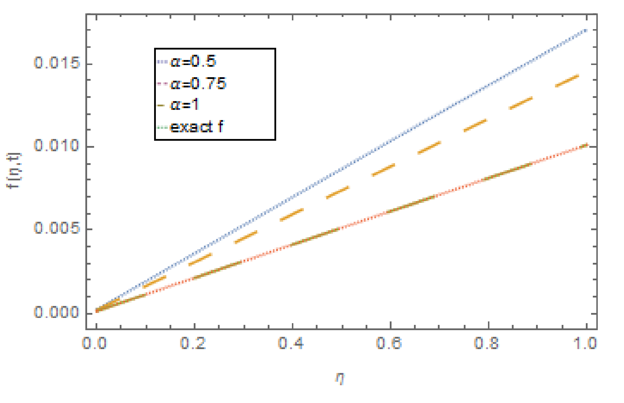
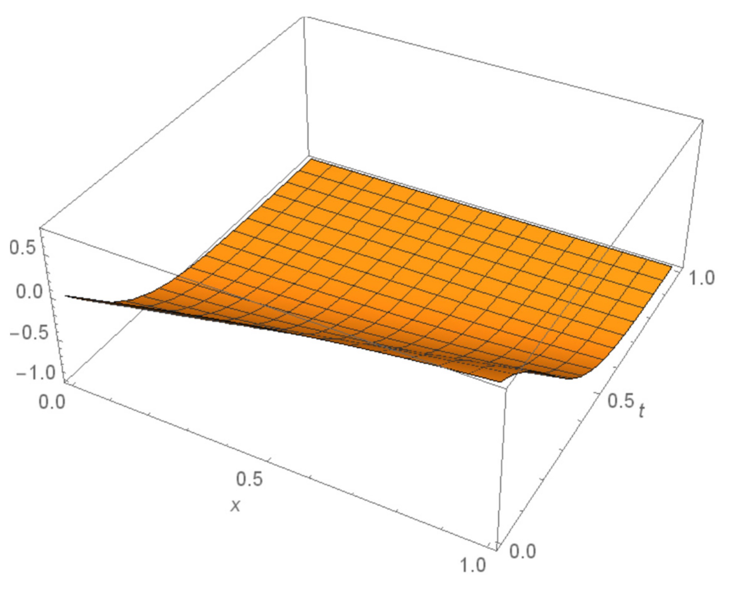
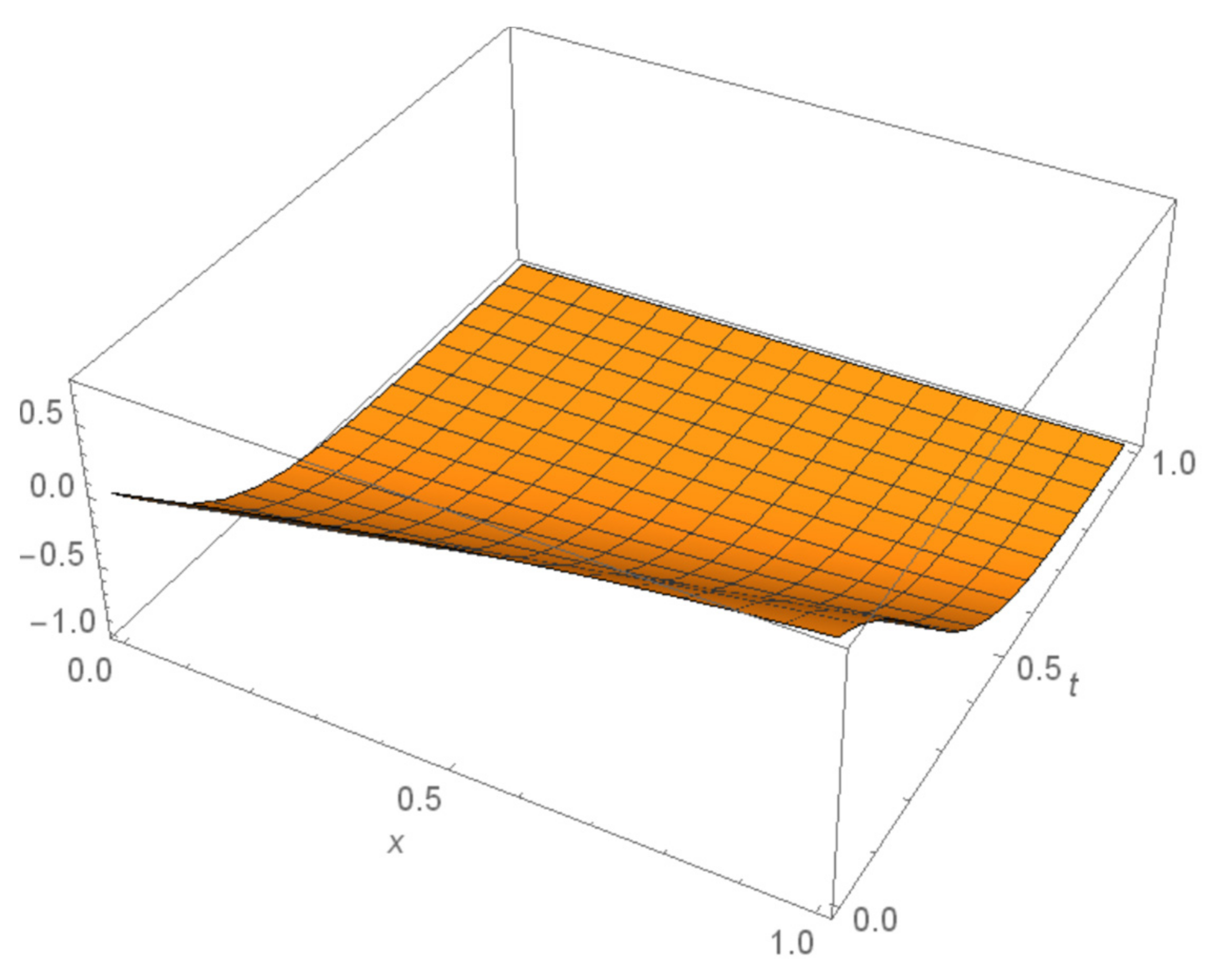
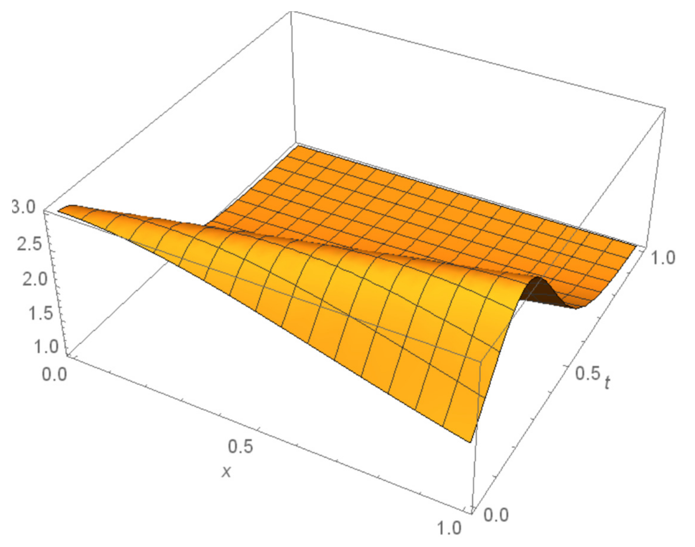
4. Numerical Examples

In this section, to illustrate the efficiency and precision of the FOAFM method, we find approximate solutions of KdV equations of fractional order. The computational work has all been done with the help of Mathematica 11.

Test Example 1: Consider the system of three KdV equations of the form:

$$\begin{array}{l}\frac{{\partial }^{\alpha }f\left(\eta ,t\right)}{\partial t^{\alpha }}=\frac{1}{2}\frac{{\partial }^{3}f\left(\eta ,t\right)}{\partial {\eta }^3}-3f\left(\eta ,t\right)\frac{\partial f\left(\eta ,t\right)}{\partial \eta }+3\frac{\partial }{\partial \eta }\left(g\left(\eta ,t\right)h\left(\eta ,t\right)\right),\\ \frac{{\partial }^{\alpha }g\left(\eta ,t\right)}{\partial t^{\alpha }}=-\frac{{\partial }^{3}g\left(\eta ,t\right)}{\partial {\eta }^3}+3f\left(\eta ,t\right)\frac{\partial g\left(\eta ,t\right)}{\partial \eta },\\ \frac{{\partial }^{\alpha }h\left(\eta ,t\right)}{\partial t^{\alpha }}=-\frac{{\partial }^{3}h\left(\eta ,t\right)}{\partial {\eta }^3}+3f\left(\eta ,t\right)\frac{\partial h\left(\eta ,t\right)}{\partial \eta }.\end{array}$$

(16)

with,

$$\begin{array}{l}f\left(\eta ,0\right)=\frac{1}{3}\left(\gamma -8l^2\right)+4l^2\tan {\mathrm{h}}^2\left(l\eta \right),\\ g\left(\eta ,0\right)=\frac{-4l^2\left(3l^2{d}_0-2\gamma d_2+4l^2{d}_2\right)}{3d_2{}^2}+\frac{4l^2}{d_2}\tan {\mathrm{h}}^2\left(l\eta \right),\\ h\left(\eta ,0\right)=d_0+d_2\tan {\mathrm{h}}^2\left(l\eta \right).\end{array}$$

(17)

The closed form solution of Equation (16) is given by [33]:

$$\begin{array}{l}f\left(\eta ,t\right)=\frac{1}{3}\left(\gamma -8l^2\right)+4l^2\tan {\mathrm{h}}^2\left(l(\eta +\gamma t)\right),\\ g\left(\eta ,t\right)=-\frac{4l^2\left(3l^2{d}_0-2\gamma d_2+4d_2{l}^2\right)}{3d_2{}^2}+\frac{4l^2}{d_2}\tan {\mathrm{h}}^2\left(l(\eta +\gamma t)\right),\\ h\left(\eta ,t\right)=d_0+d_2\tan {\mathrm{h}}^2\left(l(\eta +\gamma t)\right).\end{array}$$

(18)

We consider:

$$\begin{array}{l}{D}_1=G_1\tan \mathrm{h}\left(l\eta \right)+G_2\tan {\mathrm{h}}^2\left(l\eta \right),\\ D_2=G_3\tan {\mathrm{h}}^3\left(l\eta \right)+G_4\tan {\mathrm{h}}^4\left(l\eta \right),\\ D_3=G_5\tan {\mathrm{h}}^5\left(l\eta \right)+G_6\tan {\mathrm{h}}^6\left(l\eta \right),\end{array}$$

(19)

Zeroth Order System:

$$\frac{{\partial }^{\alpha }{f}_0}{\partial t^{\alpha }}=0,\hspace{0.17em}\hspace{0.17em}\hspace{0.17em}\hspace{0.17em}\hspace{0.17em}\hspace{0.17em}\hspace{0.17em}\hspace{0.17em}\hspace{0.17em}\frac{{\partial }^{\alpha }{g}_0}{\partial t^{\alpha }}=0,\hspace{0.17em}\hspace{0.17em}\hspace{0.17em}\hspace{0.17em}\hspace{0.17em}\hspace{0.17em}\hspace{0.17em}\hspace{0.17em}\hspace{0.17em}\frac{{\partial }^{\alpha }{h}_0}{\partial t^{\alpha }}=0,$$

(20)

with initial conditions:

$$\begin{array}{l}{f}_0\left(\eta ,0\right)=\frac{1}{3}\left(\gamma -8l^2\right)+4l^2\tan {\mathrm{h}}^2\left(l\eta \right),\\ g_0\left(\eta ,0\right)=\frac{-4l^2\left(3l^2{d}_0-2\gamma d_2+4l^2{d}_2\right)}{3d_2{}^2}+\frac{4l^2}{d_2}\tan {\mathrm{h}}^2\left(l\eta \right),\\ h_0\left(\eta ,0\right)=d_0+d_2\tan {\mathrm{h}}^2\left(l\eta \right).\end{array}$$

(21)

Its solution is:

$$\begin{array}{l}{f}_0\left(\eta ,t\right)=\frac{1}{3}\left(-8l^2+\gamma +12l^2\tan {\mathrm{h}}^2(l\eta )\right),\\ g_0\left(\eta ,t\right)=\frac{-4\left(3l^2{d}_0+4l^2{d}_2-2l^2\gamma d_2-3l^2{d}_2\tan {\mathrm{h}}^2(l\eta )\right)}{3d_2{}^2},\\ h_0\left(\eta ,t\right)=d_0+d_2\tan {\mathrm{h}}^2(l\eta ).\end{array}$$

(22)

First Order System:

$$\begin{gathered} \frac{{\partial }^{\alpha }{f}_1\left(\eta ,t\right)}{\partial t^{\alpha }}+D_1\left(\begin{array}{l}-12l^3(2\tan \mathrm{h}(l\eta )\cot \mathrm{h}(l\eta )+2\cot \mathrm{h}(l\eta )\tan \mathrm{h}(l\eta ))\\ -8l^2+\gamma +12l^2\tan {\mathrm{h}}^2(l\eta )+8l^3\tan \mathrm{h}(l\eta )\cot \mathrm{h}(l\eta )\\ -\frac{4}{3d_2}(3l^2{d}_0+4l^2{d}_2-2l^2\gamma d_2-6l^3{d}_2\tan {\mathrm{h}}^2(l\eta )\cot \mathrm{h}(l\eta ))\\ -3d_0+d_2\tan {\mathrm{h}}^2(l\eta )(-6l^3\tan {\mathrm{h}}^2(l\eta )\cot \mathrm{h}(l\eta ))\end{array}\right)+D_2=0, \\ \begin{array}{l}\frac{{\partial }^{\alpha }{g}_1\left(\eta ,t\right)}{\partial t^{\alpha }}+D_3\left(\begin{array}{l}\frac{14l^3}{d_2}(\tan \mathrm{h}(l\eta )\cot \mathrm{h}(l\eta )+\cot \mathrm{h}(l\eta )\tan \mathrm{h}(l\eta ))\\ -(-8l^2+\gamma +12l^2\tan {\mathrm{h}}^2(l\eta )(\frac{8l^3}{d_2}(\tan \mathrm{h}(l\eta )\cot \mathrm{h}(l\eta ))))\end{array}\right)+D_4=0,\\ \frac{{\partial }^{\alpha }{h}_1\left(\eta ,t\right)}{\partial t^{\alpha }}+D_5\left(\begin{array}{l}2d_2(\tan {\mathrm{h}}^2(l\eta )+\cot h^2(l\eta )-(-8k^2+\beta +12\tan {\mathrm{h}}^2(l\eta )))\\ -\frac{8}{d_2}(-3l^2\tan \mathrm{h}(l\eta )\cot \mathrm{h}(l\eta ))\end{array}\right)+D_6=0,\end{array} \end{gathered}$$

(23)

with

$$f_1\left(\eta ,0\right)=0, g_1\left(\eta ,0\right)=0, h_1\left(\eta ,0\right)=0$$

(24)

by taking $d_0=1.5,\hspace{0.17em}\hspace{0.17em}{d}_2=0.1,\hspace{0.17em}\hspace{0.17em}l=0.1,\hspace{0.17em}\gamma =1.5\hspace{0.17em}$ and using the values of Ds and $G_{ni},\hspace{0.17em}\hspace{0.17em}\hspace{0.17em}i=1,2,3\dots$

$$\begin{array}{l}{G}_1=-0.001196478535\hspace{0.17em}\hspace{0.17em}\hspace{0.17em}\hspace{0.17em}{G}_2=0.00000014578962\\ G_3=0.0001458765872\hspace{0.17em}\hspace{0.17em}\hspace{0.17em}\hspace{0.17em}{G}_4=0.00000004578561\\ G_5=0.0000457821458 \hspace{0.17em}\hspace{0.17em}{G}_6=0.00000045789630.\end{array}$$

We get

$$\begin{array}{l}{u}_1\left(\xi ,t\right)=\frac{1}{3}\left(2.14+0.32\tan {\mathrm{h}}^2(0.1\xi )\right)+80\frac{t^{\alpha }}{\alpha \mathsf{\Gamma }\left(\alpha \right)}\left[3.124586\times {10}^{-16}\sec h^2(0.1\xi )\tan \mathrm{h}\left(0.1\xi \right)\right],\hspace{0.17em}\hspace{0.17em}\hspace{0.17em}\hspace{0.17em}\hspace{0.17em}\\ v_1\left(\xi ,t\right)=-1.245786\frac{t^{\alpha }}{\alpha \mathsf{\Gamma }\left(\alpha \right)}\left(-0.00012-0.001\tan {\mathrm{h}}^2(0.1\xi )\right)\\ w_1\left(\xi ,t\right)=3.2+0.1\tan {\mathrm{h}}^2(0.1\xi )-2\frac{t^{\alpha }}{\alpha \mathsf{\Gamma }\left(\alpha \right)}\left[-3.24587\times {10}^{-28}\sec h^2(0.1\xi )\tan \mathrm{h}\left(0.1\xi \right)\right]\hspace{0.17em}\hspace{0.17em}\hspace{0.17em}\hspace{0.17em}\hspace{0.17em}\hspace{0.17em}\hspace{0.17em}\hspace{0.17em}\hspace{0.17em}\hspace{0.17em}\hspace{0.17em}\hspace{0.17em}\hspace{0.17em}\hspace{0.17em}\hspace{0.17em}\hspace{0.17em}\hspace{0.17em}\hspace{0.17em}\hspace{0.17em}\hspace{0.17em}\hspace{0.17em}\hspace{0.17em}\hspace{0.17em}\hspace{0.17em}\hspace{0.17em}\hspace{0.17em}\hspace{0.17em}\hspace{0.17em}\hspace{0.17em}\hspace{0.17em}\end{array}$$

(25)

The final solution is obtained as:

$$\begin{array}{l}f\left(\eta ,t\right)=f_0\left(\eta ,t\right)+f_1\left(\eta ,t\right),\\ g\left(\eta ,t\right)=g_0\left(\eta ,t\right)+g_1\left(\eta ,t\right),\\ h\left(\eta ,t\right)=h_0\left(\eta ,t\right)+h_1\left(\eta ,t\right).\end{array}$$

(26)

Test Example 2: MKdV equation [33]:

$$\begin{array}{l}\frac{{\partial }^{\alpha }f}{\partial t^{\alpha }}=\frac{1}{2}{f}_{\eta \eta \eta }-3f^2{f}_{\eta }+\frac{3}{2}{g}_{\eta \eta }+3f{g}_{\eta }+3f_{\eta }g-3\gamma f_{\eta },\\ \frac{{\partial }^{\alpha }g}{\partial t^{\alpha }}=-g_{\eta \eta \eta }-3g{g}_{\eta }-3f_{\eta }{g}_{\eta }+3f^2{g}_{\eta }+3\gamma v_{\eta },\end{array}$$

(27)

Subject to ICs

$$\begin{array}{l}f\left(\eta ,0\right)=l\tan \mathrm{h}\left(l\eta \right),\\ g\left(\eta ,0\right)=\frac{1}{2}\left(4l^2+\gamma \right)-2l^2\tan {\mathrm{h}}^2\left(l\eta \right).\end{array}$$

(28)

The closed form solution of the problem is given as:

$$\begin{array}{l}f\left(\eta ,t\right)=l\tan \mathrm{h}\left(l\left(x\eta \left(l^2+\frac{3}{2}l\right)t\right)\right),\\ g\left(\eta ,t\right)=\frac{1}{2}\left(4l^2+\gamma \right)-2l^2\tan {\mathrm{h}}^2\left(l\left(\eta -\left(l^2+\frac{3}{2}\gamma \right)t\right)\right).\end{array}$$

(29)

$$\begin{array}{l}{D}_1=G_{11}\tan \mathrm{h}\left(l\eta \right)+G_{12}\tan {\mathrm{h}}^2\left(l\eta \right),\\ D_2=G_{21}\tan {\mathrm{h}}^3\left(l\eta \right)+G_{22}\tan {\mathrm{h}}^4\left(l\eta \right),\\ D_3=G_{31}\tan {\mathrm{h}}^5\left(l\eta \right)+G_{32}\tan {\mathrm{h}}^6\left(l\eta \right),\end{array}$$

Zeroth Order System:

$$\frac{{\partial }^{\alpha }{f}_0}{\partial t^{\alpha }}\hspace{0.17em}\hspace{0.17em}\hspace{0.17em}\hspace{0.17em}\hspace{0.17em}\hspace{0.17em}\hspace{0.17em}\frac{{\partial }^{\alpha }{g}_0}{\partial t^{\alpha }}\hspace{0.17em}=0,\hspace{0.17em}\hspace{0.17em}$$

(30)

with initial conditions

$$\begin{array}{l}{f}_0\left(\eta ,0\right)=l\tan \mathrm{h}\left(l\eta \right),\\ g_0\left(\eta ,0\right)=\frac{1}{2}\left(4l^2+\gamma \right)-2l^2\tan {\mathrm{h}}^2\left(l\eta \right).\end{array}$$

(31)

Its solution is:

$$\begin{array}{l}{f}_0\left(\eta ,t\right)=l\tan \mathrm{h}\left(l\eta \right),\\ g_0\left(\eta ,t\right)=\frac{1}{2}\left(4l^2+\gamma \right)-2l^2\tan {\mathrm{h}}^2\left(l\eta \right).\end{array}$$

(32)

First Order System:

$$\begin{array}{l}\frac{\partial f_1\left(\eta ,t\right)}{\partial t}+D_1\left(\tan \mathrm{h}(l\eta ),\tan {\mathrm{h}}^2(l\eta ),G_{m1}\right)\left(\begin{array}{l}\frac{1}{2}{l}^2\tan \mathrm{h}(l\eta )+\left(-3l^3+6l^4\right)\tan {\mathrm{h}}^2(l\eta )\cot \mathrm{h}(l\eta )\\ +6l^4\tan {\mathrm{h}}^2(l\eta )+\left(\gamma +14l^4\right)\cot \mathrm{h}(l\eta )\end{array}\right)\\ +D_2\left(\tan \mathrm{h}(l\eta ),\tan {\mathrm{h}}^2(l\eta ),G_{n1}\right)=0,\\ \frac{\partial g_1\left(\eta ,t\right)}{\partial t}+D_3\left(\tan \mathrm{h}(l\eta ),\tan {\mathrm{h}}^2(l\eta ),E_{m2}\right)\left(\begin{array}{l}\left(-16l^3+24l^2+6\gamma -32\gamma l\right)(\tan \mathrm{h}(l\eta )\cot \mathrm{h}(l\eta )\\ +\left(8l^5-12l^3\right)\cot \mathrm{h}(l\eta )\tan {\mathrm{h}}^3(l\eta )\end{array}\right)\\ +D_4\left(\tan \mathrm{h}(l\eta ),\tan {\mathrm{h}}^2(l\eta ),G_{n2}\right)=0,\end{array}$$

(33)

with

$$f_1\left(\eta ,0\right)=0,, g_1\left(\eta ,0\right)=0$$

(34)

Its solution is obtained by using the values of Es and Gs given as:

$$\begin{gathered} \begin{array}{l}{G}_{11}=0.0458796563G_{21}=0.012478592\\ G_{12}=0.0078925631G_{22}=-0.01478965\\ G_{13}=0.0010655423G_{23}=1.015478960\\ G_{14}=0.0004102593G_{24}=0.000074890\\ G_{15}=0.0004319563G_{25}=0.000049561\\ G_{16}=0.0000012496G_{26}=0.000103581\end{array} \\ \begin{array}{l}{f}_1\left(\eta ,t\right)=\hspace{0.17em}\hspace{0.17em}\frac{t^{\alpha }}{\alpha \mathsf{\Gamma }\left(\alpha \right)}\sec h^2(0.1\eta )\left(0.00150104-0.0000230423\tan {\mathrm{h}}^2(0.1\eta )\right),\hspace{0.17em}\\ g_1\left(\eta ,t\right)=\frac{t^{\alpha }}{\alpha \mathsf{\Gamma }\left(\alpha \right)}\sec h^2(0.1\eta )\tan \mathrm{h}\left(0.1\eta \right)\left(0.0174345+0.00005366\tan {\mathrm{h}}^2(0.1\eta )\right).\hspace{0.17em}\hspace{0.17em}\hspace{0.17em}\end{array} \end{gathered}$$

(35)

The final solution is obtained as:

$$\begin{array}{l}\tilde{f}\left(\eta ,t\right)=f_0\left(\eta ,t\right)+f_1\left(\eta ,t\right),\\ \tilde{g}\left(\xi ,t\right)=g_0\left(\eta ,t\right)+g_1\left(\eta ,t\right),\end{array}$$

(36)

5. Results and Discussions

The mathematical theory of the FOAFM provides highly accurate solutions for the system of initial value problems which are presented in Section 3. We have used Mathematica 11 for our computational work. The results obtained by the FOAFM are compared with other methods available in the literature such as the HAM and OHAM, and are given in

Table 1. Comparison of solutions for $f\left(\eta ,t\right)$ at $\alpha =1$.

$\mathbf{\eta }$	HAM [33]	ClosedFormSol	OAFM	OHAM
0	0.5478591	0.5478594	0.5478594	0.5478591
20	0.5468792	0.5468793	0.5468793	0.5468792
40	0.5145785	0.5145789	0.5145789	0.5145785
60	0.5125476	0.5125478	0.5125478	0.5125476
80	0.5132221	0.5132222	0.5132222	0.5132221
100	0.5144442	0.5144444	0.5144444	0.5144442

,

Table 2. Comparison of solutions for $g\left(\eta ,t\right)$ at $\alpha =1$.

$\mathbf{\eta }$	HAM [33]	ClosedFormSol	OAFM	OHAM
0	0.334666	0.343533	0.343533	0.334666
20	0.706405	0.713534	0.713534	0.706405
40	0.734121	0.734269	0.734269	0.734121
60	0.734655	0.734659	0.734659	0.734655
80	0.734664	0.734667	0.734667	0.734664
100	0.734665	0.734667	0.734667	0.734665

and

Table 3. Comparison of solutions for $h\left(\eta ,t\right)$ at $\alpha =1$.

$\mathbf{\eta }$	OAFM	ClosedFormSol	HAM [33]	OHAM
0	1.5	1.50222	1.50221	1.50221
20	1.59392	1.59472	1.5947	1.5947
40	1.59985	1.5999	1.5998	1.5998
60	1.6	1.6	1.6	1.6
80	1.6	1.6	1.6	1.6
100	1.6	1.6	1.6	1.6

. The solutions are compared with the closed form solution revealing that the FOAFM is valid and more accurate than the HAM and OHAM. The absolute errors of the method for different values of $\alpha$ are presented in

Table 4. $AEf=\left|\left(closed\hspace{0.17em}form\hspace{0.17em}solution\right)-\left(\tilde{f}\left(\eta ,t\right)\right)\right|\hspace{0.17em}$.

$\mathbf{\eta }$	$\mathbf{\alpha }=0.25$	$\mathbf{\alpha }=0.5$	$\mathbf{\alpha }=0.75$	$\mathbf{\alpha }=1$
0	0.00012458	0.000014578	0.000000457	1.99865 × 10−18
20	0.000012456	0.000004578	0.000000457	2.99865 × 10−18
40	0.0000001245	0.0000000014	0.0000000245	1.58421 × 10−19
60	1.34118 × 10−8	5.63709 × 10−9	2.54789 × 10−10	5.90535 × 10−19
80	2.71092 × 10−10	2.3988 × 10−12	3.66673 × 10−14	2.32147 × 10−20
100	2.13366 × 10−12	4.562 × 10−14	7.54742 × 10−16	1.74665 × 10−20

,

Table 5. $AEg=\left|\left(closed\hspace{0.17em}form\hspace{0.17em}solution\right)-\left(\tilde{g}\left(\eta ,t\right)\right)\right|\hspace{0.17em}$.

$\mathbf{\eta }$	$\mathbf{\alpha }=0.25$	$\mathbf{\alpha }=0.5$	$\mathbf{\alpha }=0.75$	$\mathbf{\alpha }=1$
0	0.012458	0.164870	0.00012458	5.12478 × 10−18
20	0.012456	0.00012458	0.00004789	3.14586 × 10−19
40	0.000004578	0.000012458	0.000045786	3.24578 × 10−20
60	9.34118 × 10−8	7.63709 × 10−8	2.5478 × 10−10	2.90535 × 10−20
80	1.71092 × 10−9	1.3988 × 10−10	4.6667 × 10−12	5.32146 × 10−21
100	3.1336 × 10−10	2.562 × 10−11	8.54741 × 10−14	9.74660 × 10−21

,

Table 6. $AEh=\left|\left(closed\hspace{0.17em}form\hspace{0.17em}solution\right)-\left(\tilde{h}\left(\eta ,t\right)\right)\right|\hspace{0.17em}$.

$\mathbf{\eta }$	$\mathbf{\alpha }=0.25$	$\mathbf{\alpha }=0.5$	$\mathbf{\alpha }=0.75$	$\mathbf{\alpha }=1$
0	0.0045789	0.004578566	0.00002145	3.22115 × 10−18
20	0.000124578	0.000045789	0.000004586	5.11245 × 10−19
40	0.000000024	0.000004578	0.000004586	5.64850 × 10−20
60	1.45789 × 10−8	3.45789 × 10−8	3.4586 × 10−10	3.54691 × 10−21
80	2.45789 × 10−9	3.2145 × 10−10	3.4586 × 10−12	3.45879 × 10−21
100	3.1457 × 10−10	3.1245 × 10−11	2.3546 × 10−14	3.25460 × 10−21

,

Table 7. $AEf=\left|\left(closed\hspace{0.17em}form\hspace{0.17em}solution\right)-\left(\tilde{f}\left(\eta ,t\right)\right)\right|\hspace{0.17em}$.

$\mathbf{\eta }$	$\mathbf{\alpha }=0.25$	$\mathbf{\alpha }=0.5$	$\mathbf{\alpha }=0.75$	$\mathbf{\alpha }=1$
0	0.0164508	0.008144	0.000449177	4.55951 × 10−16
20	0.00217387	0.00190041	0.000754522	0.00008 × 10−16
40	0.000273879	0.0000265752	0.0000147276	1.59572 × 10−16
60	5.14463 × 10−6	4.83366 × 10−7	2.70061 × 10−7	2.92649 × 10−18
80	9.42707 × 10−8	8.85201 × 10−9	4.94645 × 10−9	5.36017 × 10−20
100	1.72664 × 10−9	1.6213 × 10−10	9.05975 × 10−11	9.81748 × 10−21

and

Table 8. $AEf=\left|\left(closed\hspace{0.17em}form\hspace{0.17em}solution\right)-\left(\tilde{g}\left(\eta ,t\right)\right)\right|\hspace{0.17em}$.

$\mathbf{\eta }$	$\mathbf{\alpha }=0.25$	$\mathbf{\alpha }=0.5$	$\mathbf{\alpha }=0.75$	$\mathbf{\alpha }=1$
0	0.0164508	0.008144	0.000449177	4.55951 × 10−16
20	0.00217387	0.00190041	0.000754522	0.00008 × 10−16
40	0.000273879	0.0000265752	0.0000147276	1.59572 × 10−16
60	5.14463 × 10−6	4.83366 × 10−7	2.70061 × 10−7	2.92649 × 10−18
80	9.42707 × 10−8	8.85201 × 10−9	4.94645 × 10−9	5.36017 × 10−20
100	1.72664 × 10−9	1.6213 × 10−10	9.05975 × 10−11	9.81748 × 10−21

for both problems. Figure 1, Figure 2, Figure 3, Figure 4, Figure 5 and Figure 6 show the 3D plots of exact versus approximate solutions by the proposed method for Example 1. Figure 7 shows the 2D plots of approximate solutions by the proposed method for Example 1 at different values of α. In addition, Figure 8, Figure 9, Figure 10 and Figure 11 show the 3D plots of exact versus approximate solutions by the proposed method for Example 2. Figure 12 and Figure 13 show the 2D plots of approximate solutions by the proposed method for Example 2 at different values of α. Since the absolute errors are decreasing with an increase in the value of $\alpha$, it proves that the accuracy of the method increases when the values of $\alpha$ tend to 1. The solution is again validated by comparing the solutions with closed form solutions in 3D form, as given in Figure 1, Figure 2, Figure 3, Figure 4, Figure 5, Figure 6 and Figure 8, Figure 9, Figure 10 and Figure 11. From Figure 7, Figure 12, and Figure 13 and Table 4, Table 5, Table 6, Table 7 and Table 8, it is evident that when the values of $\alpha$ are closer to 1, then, the absolute error is decreased and for $\alpha =1$, when used in the FOAFM, we get the closest result to the closed form solution. In addition, the absolute errors obtained by the FOAFM are compared with other methods in the literature and it is concluded that the FOAFM results are more accurate than the other method.

6. Conclusions

In this study, a new analytical method, namely the OAFM, is suggested for solving KdV equations. We obtained the first order series solution for the governing equations of the KdV equations and achieved the first order solution with high accuracy. For the accuracy and validity of our method, we compared the OAFM results with the results available in the literature and the numerical results obtained by using the HAM and OHAM. From the comparisons, it is concluded that the suggested method is very accurate and the good agreement of our results with the numerical results proves the validity of our method. The OAFM is applicable and is very easy in its applicability to high nonlinear initial and boundary value problems even if the nonlinear initial/boundary value problem does not contain the small parameter. As compared with other analytical methods, the OAFM is very easy in applicability and provides good results for more complex nonlinear initial/boundary value problems. The OAFM contains the optimal auxiliary constants through which we can control the convergence, as the OAFM contains the auxiliary functions $D_1,D_2,D_3,D_4$, in which the optimal constants $G_i,i=1,2,3\dots$ the control convergence parameters exist to play an important role to get the convergent solution which is obtained rigorously. The computational work in the OAFM is less than other methods and even a low specification computer can do the computational work easily. Until now, there are no limitation of this method, which enables us to implement this efficient and fast convergent method in our future work for more complex models arising from real-world problems.

References

1. Fellah, Z.E.A.; Depollier, C.; Fellah, M. Application of fractional calculus to sound wave propagation in rigid porous materials, validation via ultrasonic measurements. Acta Acustic United Acust. 2002, 88, 34–39. [Google Scholar]
2. Sebaa, N.; Fellah, Z.; Lauriks, W.; Depollier, C. Application of fractional calculus to ultrasonic wave propagation in human cancellous bone. Signal Process. 2006, 86, 2668–2677. [Google Scholar] [CrossRef]
3. Meral, F.C.; Royston, T.J.; Magin, R. Fractional calculus in viscoelastic an experimental study. Commun. Nonlinear Sci. Numer. Simul. 2010, 15, 939–945. [Google Scholar] [CrossRef]
4. Sua´rez, J.I.; Vinagre, B.M.; Calder´on, A.J.; Monje, C.A.; Chen, Y.Q. Using fractional calculus for lateral and longitudinal control of autonomous vehicles. In Lecture Notes in Computer Science; Springer: Berlin, Germany, 2004. [Google Scholar]
5. Oldham, K.B.; Spanier, J. e Fractional Calculus; Academic Press: New York, NY, USA, 1974. [Google Scholar]
6. Meerschaert, M.M.; Scheffler, H.-P.; Tadjeran, C. Finite difference methods for two-dimensional fractional dispersion equation. J. Comput. Phys. 2006, 211, 249–261. [Google Scholar] [CrossRef]
7. Metzler, R.; Klafter, J. The restaurant at the end of the random walk: Recent developments in the description of anomalous transport by fractional dynamics. J. Phys. A 2004, 37, 161–208. [Google Scholar] [CrossRef]
8. Podlubny, I. Fractional Differential Equations; Academic Press: New York, NY, USA, 1999. [Google Scholar]
9. Schneider, W.R.; Wyess, W. Fractional diffusion and wave equations. J. Math. Phys. 1989, 30, 134–144. [Google Scholar] [CrossRef]
10. Torrisi, M.; Tracina, R.; Valenti, A. A group analysis approach for a nonlinear differential system arising in diffusion phenomena. J. Math. Phys. 1996, 37, 4758–4767. [Google Scholar] [CrossRef]
11. Drzain, P.G.; Johnson, R.S. An Introduction Discussion the Theory of Solution and Its Diverse Applications; Cambridge Unversity Press: Cambridge, UK, 1989. [Google Scholar]
12. Abdel-Hamid, B. Exact solutions of some nonlinear evolution equations using symbolic computations. Comput. Math. Appl. 2000, 40, 291–302. [Google Scholar] [CrossRef] [Green Version]
13. Bluman, G.; Kumei, S. On the remarkable nonlinear diffusion equations. J. Math. Phys. 2003, 21, 1019–1023. [Google Scholar] [CrossRef]
14. Chun, L.C. Fourier series based variational iteration method for a reliable treatment of heat equations with variable coefficients. Int. J. Nonlinear Sci. Numer. Simul. 2007, 10, 1383–1388. [Google Scholar] [CrossRef]
15. Chowdhury, S.H. A comparison between the Extended homotopy perturbation method and adomian decomposition method for solving nonlinear heat transfer equations. J. Appl. Sci. 2011, 11, 1416–1420. [Google Scholar] [CrossRef]
16. Yaghoobi, H.; Tirabi, M. The application of differential transformation method to nonlinear equation arising in heat transfer. Int. Commun. Heat Mass Transf. 2011, 38, 815–820. [Google Scholar] [CrossRef]
17. Ganji, D.D. The application of He’s homotopy perturbation method to nonlinear equation arising in heat transfer. Phys. Lett. A 2006, 355, 337–341. [Google Scholar] [CrossRef]
18. Bellman, R. Perturbation techniques in Mathematics. In Physics and Engineering; Rinehart and Winston: New York, NY, USA, 1964. [Google Scholar]
19. Cole, J.D. Perturbation Methods in Applied Mathematics; Blaisedell: Waltham, MA, USA, 1968. [Google Scholar]
20. O’Malley, R.E. Introduction to Singular Perturbation; Acadmeic Press: New York, NY, USA, 1974. [Google Scholar]
21. Liao, S.J. The Proposed Homotopy Analysis Technique for the Solution of Nonlinear Problems. Ph.D. Thesis, Shanghai Jiao Tong University, Shanghai, China, 1992. [Google Scholar]
22. Marinca, V.; Herisanu, N.; Nemes, I. Optimal homotopy asymptotic method with application to thin film flow. Cent. Eur. J. Phys. 2008, 6, 648–653. [Google Scholar] [CrossRef]
23. Herisanu, N.; Marinca, V. Explicit analytical approximation to large amplitude nonlinear osciallation of a uniform contilaver beam carrying an intermediate lumped mass and rotary inertia. Meccanica 2010, 45, 847–855. [Google Scholar] [CrossRef]
24. Marinca, V.; Herisanu, N. An optimal homotopy asymptotic method applied to the steady flow of a fourth-grade fluid past a porous plate. Appl. Math. Lett. 2009, 22, 245–251. [Google Scholar] [CrossRef] [Green Version]
25. Marinca, V.; Herisanu, N.; Nemes, I. A New Analytic Approach to Nonlinear Vibration of an Electrical Machine. Proceeding Rom. Acad. 2008, 25, 9229–9236. [Google Scholar]
26. Marinca, V.; Herisanu, N. Determination of periodic solutions for the motion of a particle on a rotating parabola by means of the Optimal Homotopy Asymptotic Method. J. Sound Vib. 2009, 11, 005. [Google Scholar] [CrossRef]
27. Ullah, H.; Islam, S.; Fiza, M. An Extension of the Optimal Homotopy Asymptotic Method to Coupled Schrödinger-KdV. E Quation. Int. J. Differ. Equ. 2014, 2014, 1–12. [Google Scholar] [CrossRef]
28. Ullah, H.; Islam, S.; Idrees, M.; Arif, M. Solution of Boundary Layer Problems with Heat Transfer by Optimal Homotopy Asymptotic Method. Abstr. Appl. Anal. 2013, 2013, 1–10. [Google Scholar] [CrossRef]
29. Ullah, H.; Islam, S.; Idrees, M.; Arif, M. Application of Optimal Homotopy Asymptotic Method to Doubly Wave Solutions of the Coupled Drinfel’d-Sokolov-Wilson Equations. Math. Probl. Eng. 2013, 2013, 1–8. [Google Scholar] [CrossRef]
30. Ullah, H.; Islam, S.; Sharidan, S.; Khan, I.; Fiza, M. Formulation and application of Optimal Homotopy Asymptotic Method for coupled Differential Difference Equations. PLoS ONE 2015, 10, e0120127. [Google Scholar] [CrossRef] [PubMed]
31. Ullah, H.; Islam, S.; Khan, I.; Dennis, L.C.C.; Fiza, M. Approximate Solution of Two-Dimensional Nonlinear Wave Equation by Optimal Homotopy Asymptotic Method. Math. Probl. Eng. 2015, 2015, 1–7. [Google Scholar] [CrossRef]
32. Marinca, B.; Marinca, V. Approximate analytical solutions for thin film flow of fourth grade fluid down a vertical cylinder. Proceeding Rom. Acad. Ser. A 2018, 19, 69–76. [Google Scholar]
33. Abbasbandy, S. The application of homotopy analysis method to a generalized Hirota-Satsuama coupled KdV equations. Phys. Lett. A 2007, 361, 478–483. [Google Scholar] [CrossRef]
34. Momani, S.; Odibat, Z. Numerical comparison of method for solving linear differntial equation, of fractional order. Chaos Solitons Fractals 2007, 31, 1248–1255. [Google Scholar] [CrossRef]
35. Momani, S.; Odibat, Z. Numerical approach to differential equations of fractional order. J. Comput. Appl. Math. 2007, 207, 96–110. [Google Scholar] [CrossRef] [Green Version]
36. Odibat, Z.; Momani, S. Numerical methods for nonlinear partial differential equations of fractional order. Appl. Math. Moddeling 2008, 32, 28–39. [Google Scholar] [CrossRef] [Green Version]
37. Korteweg, D.; Vries, D.G. On the change of from of long waves advancing in a rectangular canal and on a new type of long statiionary waves. Philosphical Mag. 1895, 39, 422–428. [Google Scholar] [CrossRef]
38. Fung, M.K. KdV equation as an Euler-Poincare equation. Chin. J. Phys. 1997, 35, 789–798. [Google Scholar]
39. El-Wakil, S.A.; Abulwafa, E.M. Formulation and solution of space-time fractional Boussinesq equation. Nonlinear Dyn. 2015, 80, 167–175. [Google Scholar] [CrossRef]
40. Nazari-Golshan, N.A.; Nourazar, S.S. Effect of trapped electron on the dust ion acoustic waves in dusty plasma using time fractional modified Korteweg-de Vries equation. Phys. Plasmas 2013, 20, 103701. [Google Scholar] [CrossRef]
41. El-Shewy, E.K.; Mahmoud, A.A.; Tawfik, A.M.; Abulwafa, E.M.; Elgarayhi, A. Space—Time fractional KdV-Burgers equation for dust acoustic shock waves in dusty plasma with non-thermal ions. Chin. Phys. B 2014, 23, 070505. [Google Scholar] [CrossRef]
42. Ghosh, U.; Sengupta, S.; Sarkar, S.; Das, S. Analytical solution with tanh-method and fractional subequation method for non-linear partial differential equations and corresponding fractional differential equation composed with Jumarie fractional derivative. Int. J. Appl. Math. Stat. 2016, 54, 11–31. [Google Scholar]
43. Alzaidy, J.F. The fractional sub–equation method and exact analytical solutions for some non-linear fractional PDEs. Am. J. Math. Anal. 2013, 1, 14–19. [Google Scholar]
44. Yomba, E. The extended Fan’s sub-equation method and its application to KdV–MKdV, BKK and variant Boussinesq equations. Phys. Lett. A 2005, 336, 463–476. [Google Scholar] [CrossRef]
Figure 1. 3D plot of f ˜ η , t .
Fractalfract 06 00288 g001
Figure 2. 3D exact solution of f η , t .
Fractalfract 06 00288 g002
Figure 3. 3D plot of g ˜ η , t .
Fractalfract 06 00288 g003
Figure 4. 3D plot of exact solution of g η , t .
Fractalfract 06 00288 g004
Figure 5. 3D plot of h ˜ η , t .
Fractalfract 06 00288 g005
Figure 6. 3D plot of exact solution of h η , t .
Fractalfract 06 00288 g006
Figure 7. 2D plot of approximate solution for α .
Fractalfract 06 00288 g007
Figure 8. 3D plot of f ˜ at α = 1 .
Fractalfract 06 00288 g008
Figure 9. 3D plot of exact solution of f .
Fractalfract 06 00288 g009
Figure 10. 3D plot of g ˜ at α = 1 .
Fractalfract 06 00288 g010
Figure 11. 3D plot of exact solution.
Fractalfract 06 00288 g011
Figure 12. 2D plot of comparison of solutions.
Fractalfract 06 00288 g012
Figure 13. 2D plot of comparison of solutions.
Fractalfract 06 00288 g013