
An Averaging Principle for Stochastic Fractional Differential Equations Driven by fBm Involving Impulses


Abstract
:1. Introduction
- We propose an effective approximation for the original system (1); hence, the complexity of ISFDEs under fBm can be reduced.
- The problem of no match on each of the time scales of the standard stochastic fractional differential equations is pointed out and corrected.
- The obtained averaging principle is valid for stochastic fractional differential equations driven by fBm; that is, our results are new even for non-impulsive SFDEs with fBm.
- We present a method to estimate the impulsive terms, which is helpful to develop averaging principles for different types of ISDEs.
2. Preliminary
- (i)
- is -adapted, and has càdlàg path a.e. on ;
- (ii)
- for all meets the integral equation below:
3. Main Results
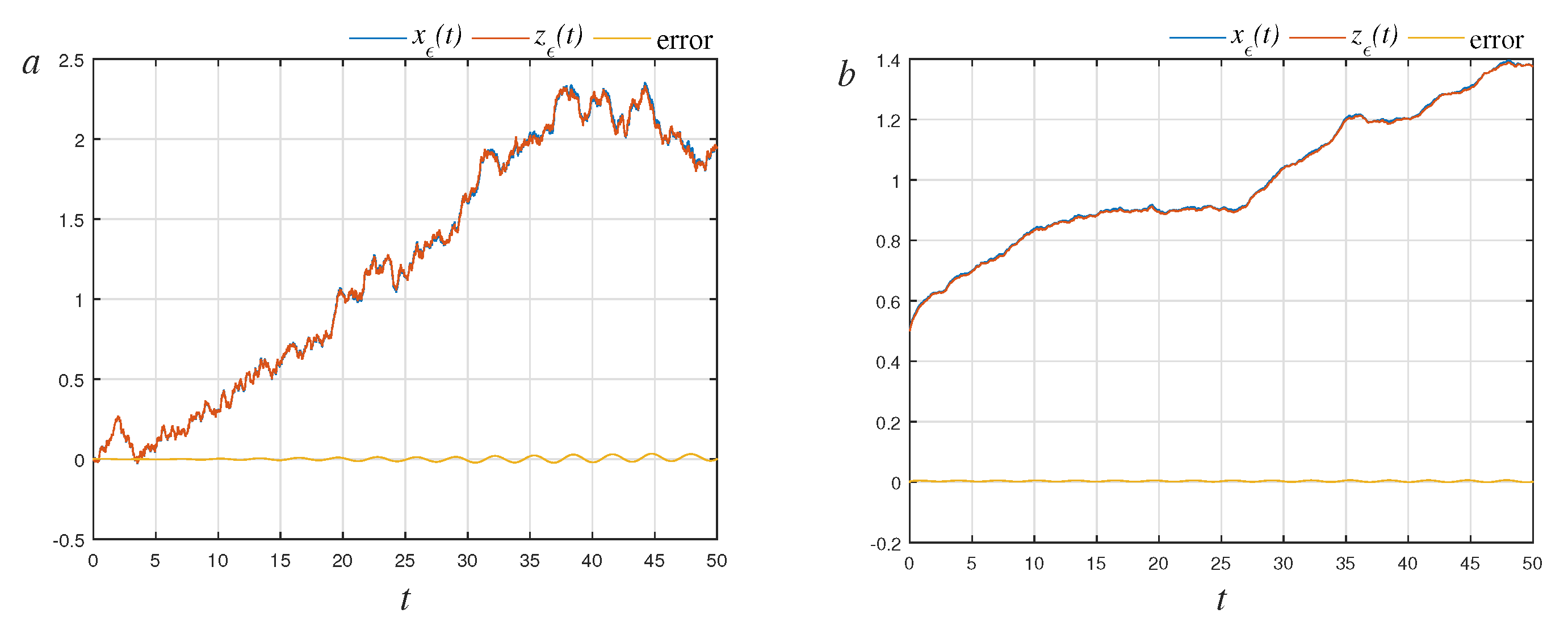
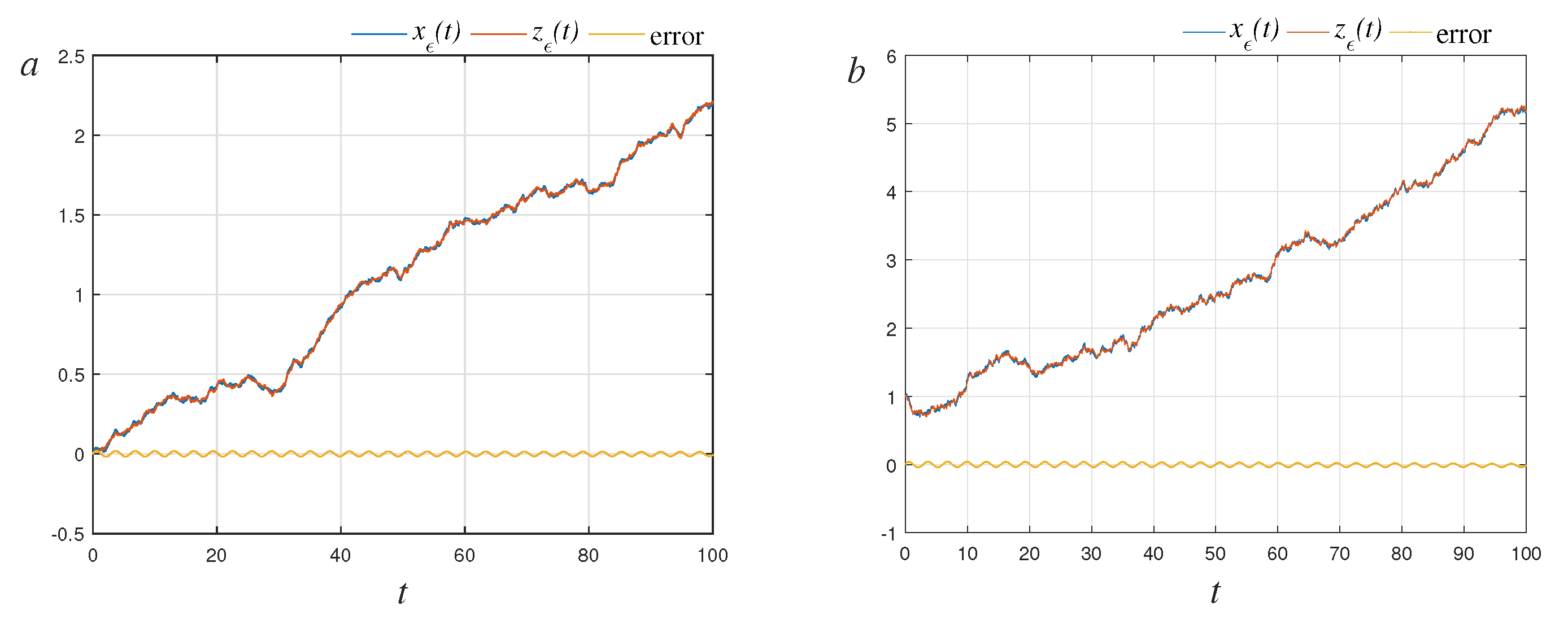
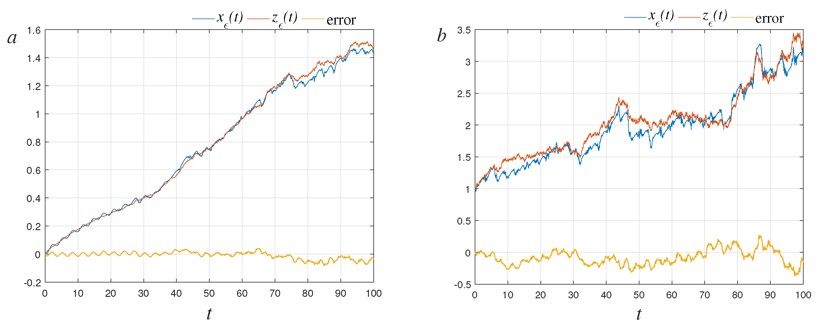
4. Example
Author Contributions
Funding
Institutional Review Board Statement
Informed Consent Statement
Data Availability Statement
Conflicts of Interest
References
- Ragusa, M.A. On weak solutions of ultraparabolic equations. Nonlinear Anal. Theor. 2001, 47, 503–511. [Google Scholar] [CrossRef]
- Machado, J.T.; Mainardi, F.; Kiryakova, V. Fractional calculus: Quo vadimus? (Where are we going?). Fract. Calc. Appl. Anal. 2015, 18, 495–526. [Google Scholar] [CrossRef]
- Khan, I.; Ullah, H.; AlSalman, H. Fractional analysis of MHD boundary layer flow over a stretching sheet in porous medium: A new stochastic Method. J. Func. Spaces 2021, 2021, 5844741. [Google Scholar] [CrossRef]
- Yang, M. (Weighted pseudo) almost automorphic solutions in distribution for fractional stochastic differential equations driven by levy noise. Filomat 2021, 35, 2403–2424. [Google Scholar] [CrossRef]
- Sakthivel, R.; Revathib, P.; Ren, Y. Existence of solutions for nonlinear fractional stochastic differential equations. Nonlinear Anal. Theor. 2013, 81, 70–86. [Google Scholar] [CrossRef]
- Kamrani, M. Numerical solution of stochastic fractional differential equations. Numer. Algor. 2015, 68, 81–93. [Google Scholar] [CrossRef]
- Lakshmikantham, V.; Bainov, D.D.; Simeonov, P.S. Theory of Impulsive Differential Equations; World Scientific: Singapore, 1989. [Google Scholar]
- Perestyuk, N.A.; Plotnikov, V.A.; Samoilenko, A.M.; Skripnik, N.V. Differential Equations with Impulse Effects: Multivalued Right-Hand Sides with Discontinuities; Walter de Gruyter: Berlin, Germany, 2011. [Google Scholar]
- Hu, Y.; Øksendal, B. Fractional white noise calculus and applications to finance. Infin. Dimens. Anal. Quantum Probab. Relat. Top. 2003, 6, 1–32. [Google Scholar] [CrossRef]
- Liu, J.; Yan, L.; Cang, Y. On a jump-type stochastic fractional partial differential equation with fractional noises. Nonlinear Anal. Theor. 2012, 75, 6060–6070. [Google Scholar] [CrossRef]
- Li, K. Stochastic delay fractional evolution equations driven by fractional Brownian motion. Math. Methods Appl. Sci. 2015, 38, 1582–1591. [Google Scholar] [CrossRef] [Green Version]
- Xu, L.; Li, Z. Stochastic fractional evolution equations with fractional Brownian motion and infinite delay. Appl. Math. Comput. 2018, 336, 36–46. [Google Scholar] [CrossRef]
- Chadha, A.; Pandey, D.N. Existence results for an impulsive neutral stochastic fractional integro-differential equation with infinite delay. Nonlinear. Anal. Theor. 2015, 128, 149–175. [Google Scholar] [CrossRef]
- Dhayal, R.; Malik, M.; Abbas, S. Approximate controllability for a class of non-instantaneous impulsive stochastic fractional differential equation driven by fractional Brownian motion. Differ. Equ. Dyn. Syst. 2021, 29, 175–191. [Google Scholar] [CrossRef]
- Pedjeu, J.C.; Ladde, G.S. Stochastic fractional differential equations: Modeling, method and analysis. Chaos Solitons Fract. 2012, 45, 279–293. [Google Scholar] [CrossRef]
- Abouagwa, M.; Cheng, F.; Li, J. Impulsive stochastic fractional differential equations driven by fractional Brownian motion. Adv. Differ. Equ. 2020, 2020, 57. [Google Scholar] [CrossRef]
- Khasminskii, R.Z. A limit theorem for the solution of differential equations with random right-hand sides. Theory Probab. Appl. 1963, 11, 390–405. [Google Scholar] [CrossRef]
- Roberts, J.B.; Spanos, P.D. Stochastic averaging: An approximate method of solving random vibration problems. Int. J. Nonlin. Mech. 1986, 21, 111–134. [Google Scholar] [CrossRef]
- Zhu, W.Q. Stochastic Averaging Methods in Random Vibration. Appl. Mech. Rev. 1988, 41, 189–199. [Google Scholar] [CrossRef]
- Xu, Y.; Pei, B.; Guo, R. Stochastic averaging for slow-fast dynamical systems with fractional Brownian motion. Discret. Contin. Dyn. Syst. B 2015, 20, 2257–2267. [Google Scholar] [CrossRef]
- Xu, Y.; Pei, B.; Wu, J.L. Stochastic averaging principle for differential equations with non-Lipschitz coefficients driven by fractional Brownian motion. Stoch. Dyn. 2017, 17, 1750013. [Google Scholar] [CrossRef] [Green Version]
- Ma, S.; Kang, Y.M. Periodic averaging method for impulsive stochastic differential equations with Lévy noise. Appl. Math. Lett. 2019, 93, 91–97. [Google Scholar] [CrossRef]
- Khalaf, A.D.; Abouagwa, M.; Wang, X. Periodic averaging method for impulsive stochastic dynamical systems driven by fractional Brownian motion under non-Lipschitz condition. Adv. Differ. Equ. 2019, 526. [Google Scholar] [CrossRef] [Green Version]
- Cui, J.; Bi, N. Averaging principle for neutral stochastic functional differential equations with impulses and non-Lipschitz coefficients. Stat. Probabil. Lett. 2020, 163, 108775. [Google Scholar] [CrossRef]
- Wang, P.; Xu, Y. Periodic averaging principle for neutral stochastic delay differential equations with impulses. Complexity 2020, 2020, 6731091. [Google Scholar] [CrossRef]
- Liu, J.K.; Xu, W.; Guo, Q. Averaging principle for impulsive stochastic partial differential equations. Stoch. Dynam. 2021, 21, 2150014. [Google Scholar] [CrossRef]
- Xu, W.J.; Duan, J.Q.; Xu, W. An averaging principle for fractional stochastic differential equations with lévy noise. Chaos Interdiscip. J. Nonlinear Sci. 2020, 30, 083126. [Google Scholar] [CrossRef] [PubMed]
- Abouagwa, M.; Li, J. Approximation properties for solutions to Itô–Doob stochastic fractional differential equations with non-Lipschitz coefficients. Stoch. Dynam. 2019, 19, 1950029. [Google Scholar] [CrossRef]
- Luo, D.F.; Zhu, Q.X.; Luo, Z.G. An averaging principle for stochastic fractional differential equations with time-delays. Appl. Math. Lett. 2020, 105, 106290. [Google Scholar] [CrossRef]
- Shen, G.J.; Xiao, R.D.; Yin, X.W. Averaging principle and stability of hybrid stochastic fractional differential equations driven by Lévy noise. Int. J. Syst. Sci. 2020, 51, 2115–2133. [Google Scholar] [CrossRef]
- Guo, Z.K.; Hu, J.H.; Yuan, C.G. Averaging principle for a type of Caputo fractional stochastic differential equations. Chaos Interdiscip. J. Nonlinear Sci. 2021, 31, 053123. [Google Scholar] [CrossRef]
- Liu, J.K.; Xu, W. An averaging result for impulsive fractional neutral stochastic differential equations. Appl. Math. Lett. 2021, 114, 106892. [Google Scholar] [CrossRef]
- Russo, F.; Vallois, P. Forward, backward and symmetric stochastic integration. Probab. Theory Relat. Fields 1993, 97, 403–421. [Google Scholar] [CrossRef]
- Biagini, F.; Hu, Y.Z.; Øksendal, B.; Zhang, T.S. Stochastic Calculus for Fractional Brownian Motion and Applications; Springer: London, UK, 2008. [Google Scholar]
- Shen, L.J.; Sun, J.T. Existence and uniqueness of mild solutions for nonlinear stochastic impulsive differential equation. Abstr. Appl. Anal. 2011, 2011, 439724. [Google Scholar] [CrossRef] [Green Version]


Publisher’s Note: MDPI stays neutral with regard to jurisdictional claims in published maps and institutional affiliations. |
© 2022 by the authors. Licensee MDPI, Basel, Switzerland. This article is an open access article distributed under the terms and conditions of the Creative Commons Attribution (CC BY) license (https://creativecommons.org/licenses/by/4.0/).
Share and Cite
Liu, J.; Wei, W.; Xu, W. An Averaging Principle for Stochastic Fractional Differential Equations Driven by fBm Involving Impulses. Fractal Fract. 2022, 6, 256. https://doi.org/10.3390/fractalfract6050256
Liu J, Wei W, Xu W. An Averaging Principle for Stochastic Fractional Differential Equations Driven by fBm Involving Impulses. Fractal and Fractional. 2022; 6(5):256. https://doi.org/10.3390/fractalfract6050256
Chicago/Turabian StyleLiu, Jiankang, Wei Wei, and Wei Xu. 2022. "An Averaging Principle for Stochastic Fractional Differential Equations Driven by fBm Involving Impulses" Fractal and Fractional 6, no. 5: 256. https://doi.org/10.3390/fractalfract6050256
APA StyleLiu, J., Wei, W., & Xu, W. (2022). An Averaging Principle for Stochastic Fractional Differential Equations Driven by fBm Involving Impulses. Fractal and Fractional, 6(5), 256. https://doi.org/10.3390/fractalfract6050256