
Cluster Analysis on Locally Asymptotically Self-Similar Processes with Known Number of Clusters


Abstract
1. Introduction
2. A Class of Locally Asymptotically Self-Similar Processes
- denotes a complex-valued Gaussian measure (see Proposition 2.1 in [43]) satisfyingfor anywith being the Fourier transform of f and being a standard Brownian motion.
- The Hurst functional parameter is a Hölder function with exponent . Subject to this constraint the paths of mBm are almost surely continuous functions.
3. Clustering Stochastic Processes
3.1. Covariance-Based Dissimilarity Measure between Autocovariance Ergodic Processes
- For any integers , , is the shortcut notation of the row vector .
- The distance ρ between two equal-sized covariance matrixes denotes the Frobenius norm of . Recall that for a matrix , its Frobenius norm is defined by where for each , denotes the -coefficient of .
- For , and , denotes the empirical covariance matrix of the process s path , which is given below:where denotes the transpose of a matrix.
3.2. Covariance-Based Dissimilarity Measure between Locally Asymptotically Self-Similar Processes
- L is chosen from .
- , are the localized increment paths defined as in (29). Heuristically speaking, for , computes the “distance” between the two covariance structures (of the increments of ) indexed by the time in the neighborhood of , and averages the above distances. It is worth noting that the value K describes the “sample size” used to approximate each local distance . Therefore, its value should be picked neither too large nor too small and it can depend on n. It is suggested that in order that the result of estimating the dissimilarity measure is acceptable. The largest value one can set for K is (correspondingly, ).
4. Approximately Asymptotically Consistent Algorithms
4.1. Offline and Online Algorithms
| Algorithm 1: Offline clustering. |
 |
| Algorithm 2: Online clustering. |
 |
4.2. Computational Complexity and Consistency of the Algorithms
- Upper bound of: Similar to how (43) is derived, we use the triangle inequalities (Remark 5) and (39) to obtain:Since the clusters are sorted in the order of appearance of the distinct process covariance structures, we have for all and , where we recall that the index is defined in (50). It follows from (55), the fact that and (53) thatFor , by (54), the triangle inequality, (49) and (56), we have
- Upper bound of the first term: Using (53) and the fact that we obtain
- Upper bound of the second term: Recall that for all and . Therefore, by (52) and the fact that for every we have
5. Tests on Simulated Data: Clustering Multifractional Brownian Motions
5.1. Efficiency Improvement: -Transformation
5.2. Simulation Methodology
5.3. Synthetic Datasets
- Case 1 (Monotonic function): The general form is taken to bewhere is a fixed integer and different values of h correspond to different clusters. We then predetermine five clusters with various hs to separate different clusters. In this study, we set , and . The trajectories of the five functional forms of in different clusters are illustrated in the left graph of Figure 1.
- Case 2 (Periodic function): The general form is taken to bewhere different values of h lead to different clusters. Specifically, we take , and . The trajectories of the corresponding five functional forms of are illustrated in the left graph of Figure 2.
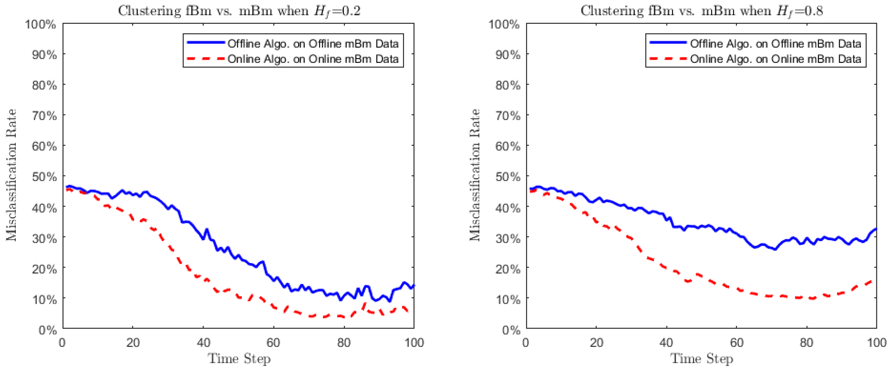
- Case 3 (Small turbulence on ): We proceed to examine if the proposed algorithm has the capacity of distinguishing processes with very similar behaviors. To this end we take consider clustering an fBm with Hurst parameter , and an mBm with the Hurst functional parameterWe perform the tests using two values of : (i) and (ii) . In both cases, the index of the corresponding mBm is regarded to be plus some noise.
- 1.
- For , simulate 20 mBm paths in group i (corresponding to ), each path is with length of 305. Then the total number of paths . To be more explicit we denote bywhere each row is an mBm discrete-time path. For , the data from the ith group are given as:
- 2.
- At each , we observe the first values of each path, i.e.,
- 1.
- 2.
- At each and , we observe the following dataset in the ith group:where
- s are the -coefficients in given in (75).
- denotes the number of paths in the ith group. Here denotes the floor number. That is, starting from 6 paths in each group, 1 new path will be added into each group as t increases by 10.
- , with . This means each path observes three new values as t increases by 1.
5.4. Experimental Results
- (1)
- Both algorithms attempt to be consistent in their circumstances, as the time t increases, in the sense that the corresponding misclassification rates decrease to 0.
- (2)
- Clustering mBms are asymptotically equivalent to clustering their tangent processes’ increments.
- (3)
- The online algorithm seems to have an overall better performance: its misclassification rates are 5– lower than that of offline algorithm. The reason may be that at early time steps the differences among the s are not significant. Unlike the offline clustering algorithm, the online one is flexible enough to catch these small differences.
- (1)
- Both misclassification rates of the clustering algorithms have generally a declining trend as time increases.
- (2)
- As the differences among the periodic function s values go up and down, the misclassification rates go down and up accordingly.
- (3)
- The online clustering algorithm has an overall worse performance than the offline one. This may be because starting from the differences among s become significantly large. In this situation, the offline clustering algorithm can better catch these differences, since it has a larger sample size (20 paths in each group) than the online one.
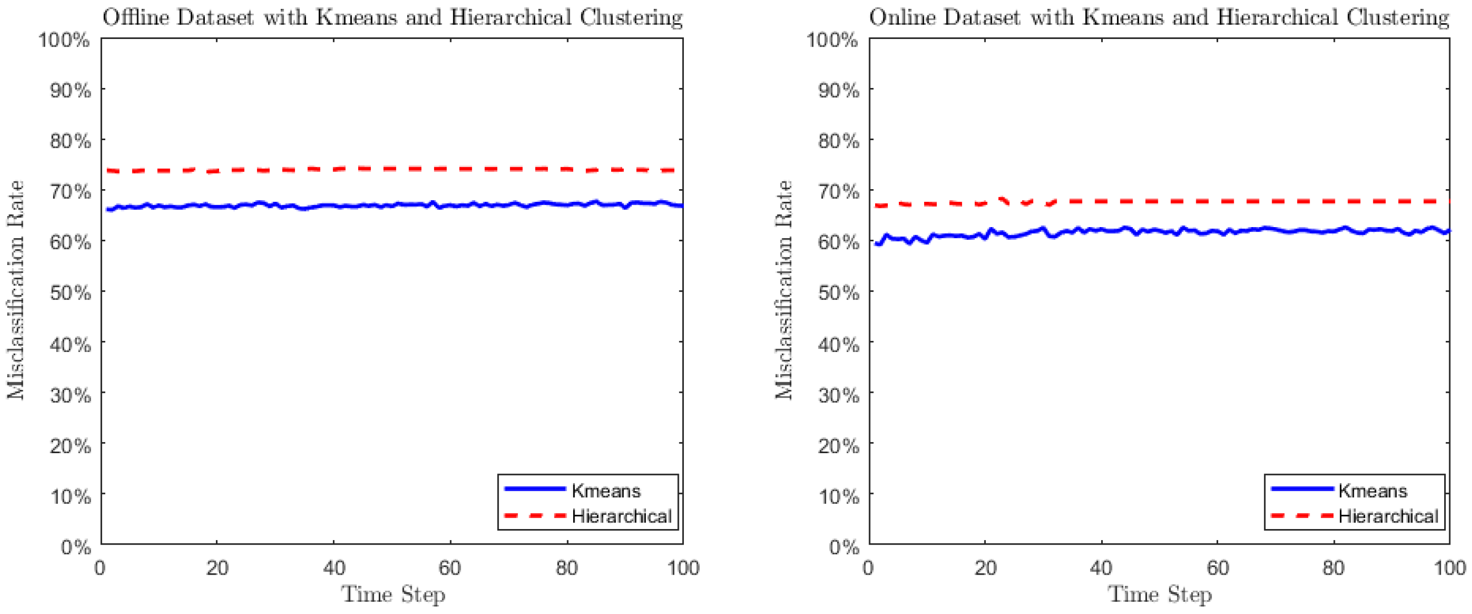
5.5. Comparison to Traditional Approaches Designed for Clustering Finite-Dimensional Vectors
6. Real World Application: Clustering Global Financial Markets
6.1. Motivation
6.2. Data and Methodology
- Equity indexes returns: We cluster the global stock indexes based on their empirical time-varying covariance structure. We use Algorithms 1 and 2 as the clustering approach. We select the index constituents of MSCI ACWI (All Country World Index) as the underlying stochastic processes in the datasets for clustering analysis. Each of the indexes is a realized path representing the historical monthly returns of the underlying economic entities. MSCI ACWI is the leading global equity market index and covers more than 85% of the market capitalization of the global stock market (As of December 2018, as reported on https://www.msci.com/acwi, accessed on 1 January 2022).
- Sovereign CDS spreads: We cluster the sovereign credit default swap (CDS) spreads of global economic entities. The sovereign CDS is an insurance-like financial product that provides default protection of treasury bonds for the economic entity (e.g., the government). The CDS spread reflects the cost to insurer of the exposure on a sovereign entity’s default. We select a five-year sovereign CDS spread as the indicator of sovereign credit risk, as the five-year product has the best liquidity on the CDS market. We overlap the sample of economic entities between the stock and CDS datasets, and the same set of underlying economics entities are present in the clustering analysis. Our CDS data source is Bloomberg.
6.3. Clustering Results
7. Conclusions and Future Prospects
- (1)
- Given their flexibility, our algorithms are applicable to clustering any distribution stationary ergodic processes with finite variances, any autocovariance ergodic processes, and locally asymptotically self-similar processes whose tangent processes have autocovariance ergodic increments. Multifractional Brownian motion (mBm) is an excellent representative of the latter class of processes.
- (2)
- Our algorithms are efficient enough in terms of their computational complexity. A simulation study is performed on clustering mBm. The results show that both offline and online algorithms are approximately asymptotically consistent.
- (3)
- Our algorithms are successfully applied to cluster the real world financial time series (equity returns and sovereign CDS spreads) via the development level and via regions. The outcomes are self-consistent with the financial markets behavior and they reveal the level of impact between the economic development and regions on equity returns.
- (1)
- The clustering framework proposed in our paper only focuses on the cases where the true number of clusters is known. The problem for which is supposed to be unknown remains open.
- (2)
- If we drop the Gaussianity assumption, the class of stationary incremental self-similar processes becomes much larger. This will yield an introduction to a more general class of locally asymptotically self-similar processes, whose autocovariances do not exist. This class includes linear multifractional stable motion [55,56] as a paradigmatic example. Cluster analysis of such stable processes will no doubt lead to a wide range of applications, especially when the process distributions exhibit heavy-tailed phenomena. Neither the distribution dissimilarity measure introduced in [12] nor the covariance-based dissimilarity measures used in this paper would work in this case, hence new techniques are required to cluster such processes, such as considering replacing the covariances with covariations [35] or symmetric covariations [57] in the dissimilarity measures.
Author Contributions
Funding
Institutional Review Board Statement
Informed Consent Statement
Data Availability Statement
Acknowledgments
Conflicts of Interest
Abbreviations
| fBm | fractional Brownian motion |
| mBm | multifractional Brownian motion |
| gBm | geometric Brownian motion |
References
- Cotofrei, P. Statistical temporal rules. In Proceedings of the 15th Conference on Computational Statistics–Short Communications and Posters, Berlin, Germany, 24–28 August 2002. [Google Scholar]
- Harms, S.K.; Deogun, J.; Tadesse, T. Discovering sequential association rules with constraints and time lags in multiple sequences. In International Symposium on Methodologies for Intelligent Systems; Springer: Berlin/Heidelberg, Germany, 2002; pp. 432–441. [Google Scholar]
- Jin, X.; Lu, Y.; Shi, C. Distribution discovery: Local analysis of temporal rules. In Pacific-Asia Conference on Knowledge Discovery and Data Mining; Springer: Berlin/Heidelberg, Germany, 2002; pp. 469–480. [Google Scholar]
- Jin, X.; Wang, L.; Lu, Y.; Shi, C. Indexing and mining of the local patterns in sequence database. In International Conference on Intelligent Data Engineering and Automated Learning; Springer: Berlin/Heidelberg, Germany, 2002; pp. 68–73. [Google Scholar]
- Keogh, E.; Kasetty, S. On the need for time series data mining benchmarks: A survey and empirical demonstration. Data Min. Knowl. Discov. 2003, 7, 349–371. [Google Scholar] [CrossRef]
- Lin, J.; Keogh, E.; Lonardi, S.; Patel, P. Finding motifs in time series. In Proceedings of the 2nd Workshop on Temporal Data Mining, Edmonton, AB, Canada, 23–26 July 2002; pp. 53–68. [Google Scholar]
- Li, C.S.; Yu, P.S.; Castelli, V. MALM: A framework for mining sequence database at multiple abstraction levels. In Proceedings of the Seventh International Conference on Information and Knowledge Management, Bethesda, MA, USA, 2–7 November 1998; pp. 267–272. [Google Scholar]
- Bradley, P.S.; Fayyad, U.M. Refining Initial Points for K-Means Clustering. ICML 1998, 98, 91–99. [Google Scholar]
- Keogh, E.; Chakrabarti, K.; Pazzani, M.; Mehrotra, S. Dimensionality reduction for fast similarity search in large time series databases. Knowl. Inf. Syst. 2001, 3, 263–286. [Google Scholar] [CrossRef]
- Java, A.; Perlman, E.S. Predictive Mining of Time Series Data. Bull. Am. Astron. Soc. 2002, 34, 741. [Google Scholar]
- Khaleghi, A.; Ryabko, D.; Mary, J.; Preux, P. Online clustering of processes. In Proceedings of the Fifteenth International Conference on Artificial Intelligence and Statistics, La Palma, Canary Islands, 21–23 April 2012; pp. 601–609. [Google Scholar]
- Khaleghi, A.; Ryabko, D.; Mary, J.; Preux, P. Consistent algorithms for clustering time series. J. Mach. Learn. Res. 2016, 17, 1–32. [Google Scholar]
- Peng, Q.; Rao, N.; Zhao, R. Covariance-based dissimilarity measures applied to clustering wide-sense stationary ergodic processes. Mach. Learn. 2019, 108, 2159–2195. [Google Scholar] [CrossRef]
- Comte, F.; Renault, E. Long memory in continuous-time stochastic volatility models. Math. Financ. 1998, 8, 291–323. [Google Scholar] [CrossRef]
- Bianchi, S.; Pianese, A. Multifractional properties of stock indices decomposed by filtering their pointwise Hölder regularity. Int. J. Theor. Appl. Financ. 2008, 11, 567–595. [Google Scholar] [CrossRef]
- Bianchi, S.; Pantanella, A.; Pianese, A. Modeling and simulation of currency exchange rates using multifractional process with random exponent. Int. J. Model. Optim. 2012, 2, 309–314. [Google Scholar] [CrossRef]
- Bertrand, P.R.; Hamdouni, A.; Khadhraoui, S. Modelling NASDAQ series by sparse multifractional Brownian motion. Methodol. Comput. Appl. Probab. 2012, 14, 107–124. [Google Scholar] [CrossRef]
- Bianchi, S.; Pantanella, A.; Pianese, A. Modeling stock prices by multifractional Brownian motion: An improved estimation of the pointwise regularity. Quant. Financ. 2013, 13, 1317–1330. [Google Scholar] [CrossRef]
- Bianchi, S.; Frezza, M. Fractal stock markets: International evidence of dynamical (in) efficiency. Chaos Interdiscip. J. Nonlinear Sci. 2017, 27, 071102. [Google Scholar] [CrossRef] [PubMed]
- Pianese, A.; Bianchi, S.; Palazzo, A.M. Fast and unbiased estimator of the time-dependent Hurst exponent. Chaos Interdiscip. J. Nonlinear Sci. 2018, 28, 031102. [Google Scholar] [CrossRef] [PubMed]
- Marquez-Lago, T.T.; Leier, A.; Burrage, K. Anomalous diffusion and multifractional Brownian motion: Simulating molecular crowding and physical obstacles in systems biology. IET Syst. Biol. 2012, 6, 134–142. [Google Scholar] [CrossRef] [PubMed]
- Song, W.; Cattani, C.; Chi, C.H. Multifractional Brownian motion and quantum-behaved particle swarm optimization for short term power load forecasting: An integrated approach. Energy 2020, 194. [Google Scholar] [CrossRef]
- Sikora, G. Statistical test for fractional Brownian motion based on detrending moving average algorithm. Chaos Solitons Fractals 2018, 116, 54–62. [Google Scholar] [CrossRef]
- Balcerek, M.; Burnecki, K. Testing of fractional Brownian motion in a noisy environment. Chaos Solitons Fractals 2020, 140, 110097. [Google Scholar] [CrossRef]
- Balcerek, M.; Burnecki, K. Testing of multifractional Brownian motion. Entropy 2020, 22, 1403. [Google Scholar] [CrossRef]
- Jin, S.; Peng, Q.; Schellhorn, H. Estimation of the pointwise Hölder exponent of hidden multifractional Brownian motion using wavelet coefficients. Stat. Inference Stoch. Process. 2018, 21, 113–140. [Google Scholar] [CrossRef]
- Peng, Q.; Zhao, R. A general class of multifractional processes and stock price informativeness. Chaos Solitons Fractals 2018, 115, 248–267. [Google Scholar] [CrossRef]
- Vu, H.T.; Richard, F.J. Statistical tests of heterogeneity for anisotropic multifractional Brownian fields. Stoch. Process. Their Appl. 2020, 130, 4667–4692. [Google Scholar] [CrossRef]
- Bicego, M.; Trudda, A. 2D shape classification using multifractional Brownian motion. In Joint IAPR International Workshops on Statistical Techniques in Pattern Recognition (SPR) and Structural and Syntactic Pattern Recognition (SSPR); Springer: Berlin/Heidelberg, Germany, 2008; pp. 906–916. [Google Scholar]
- Kirichenko, L.; Radivilova, T.; Bulakh, V. Classification of fractal time series using recurrence plots. In Proceedings of the 2018 International Scientific-Practical Conference Problems of Infocommunications. Science and Technology (PIC S&T), Kharkiv, Ukraine, 9–12 October 2018; pp. 719–724. [Google Scholar]
- Krengel, U. Ergodic Theorems; de Gruyter Studies in Mathematics; de Gruyter: Berlin, Germany, 1985. [Google Scholar]
- Grazzini, J. Analysis of the emergent properties: Stationarity and ergodicity. J. Artif. Soc. Soc. Simul. 2012, 15, 7. [Google Scholar] [CrossRef]
- Samorodnitsky, G. Extreme value theory, ergodic theory and the boundary between short memory and long memory for stationary stable processes. Ann. Probab. 2004, 32, 1438–1468. [Google Scholar] [CrossRef]
- Boufoussi, B.; Dozzi, M.; Guerbaz, R. Path properties of a class of locally asymptotically self-similar processes. Electron. J. Probab. 2008, 13, 898–921. [Google Scholar] [CrossRef]
- Samorodnitsky, G.; Taqqu, M.S. Stable Non-Gaussian Random Processes: Stochastic Models with Infinite Variance; Chapman & Hall: New York, NY, USA, 1994. [Google Scholar]
- Embrechts, P.; Maejima, M. An introduction to the theory of self-similar stochastic processes. Int. J. Mod. Phys. B 2000, 14, 1399–1420. [Google Scholar] [CrossRef]
- Embrechts, P.; Maejima, M. Selfsimilar Processes; Princeton Series in Applied Mathematics; Princeton University Press: Princeton, NJ, USA, 2002. [Google Scholar]
- Falconer, K. Tangent fields and the local structure of random fields. J. Theor. Probab. 2002, 15, 731–750. [Google Scholar] [CrossRef]
- Falconer, K. The local structure of random processes. J. Lond. Math. Soc. 2003, 67, 657–672. [Google Scholar] [CrossRef]
- Mandelbrot, B.B.; Van Ness, J.W. Fractional Brownian motions, fractional noises and applications. SIAM Rev. 1968, 10, 422–437. [Google Scholar] [CrossRef]
- Peltier, R.F.; Lévy-Véhel, J. Multifractional Brownian Motion: Definition and Preliminary Results; Technical Report 2645; Institut National de Recherche en Informatique et en Automatique, INRIA: Roquecourbe, France, 1995. [Google Scholar]
- Benassi, A.; Jaffard, S.; Roux, D. Elliptic Gaussian random processes. Revista Matemática Iberoamericana 1997, 13, 19–90. [Google Scholar] [CrossRef]
- Stoev, S.A.; Taqqu, M.S. How rich is the class of multifractional Brownian motions? Stoch. Process. Their Appl. 2006, 116, 200–221. [Google Scholar] [CrossRef]
- Ayache, A.; Véhel, J.L. On the identification of the pointwise Hölder exponent of the generalized multifractional Brownian motion. Stoch. Process. Their Appl. 2004, 111, 119–156. [Google Scholar] [CrossRef]
- Ayache, A.; Taqqu, M.S. Multifractional processes with random exponent. Publicacions Matemàtiques 2005, 49, 459–486. [Google Scholar] [CrossRef]
- Bianchi, S.; Pantanella, A. Pointwise regularity exponents and well-behaved residuals in stock markets. Int. J. Trade Econ. Financ. 2011, 2, 52–60. [Google Scholar] [CrossRef]
- Cadoni, M.; Melis, R.; Trudda, A. Financial crisis: A new measure for risk of pension fund portfolios. PLoS ONE 2015, 10, e0129471. [Google Scholar] [CrossRef] [PubMed]
- Frezza, M. Modeling the time-changing dependence in stock markets. Chaos Solitons Fractals 2012, 45, 1510–1520. [Google Scholar] [CrossRef]
- Frezza, M.; Bianchi, S.; Pianese, A. Forecasting Value-at-Risk in turbulent stock markets via the local regularity of the price process. Comput. Manag. Sci. 2022, 19, 99–132. [Google Scholar] [CrossRef]
- Garcin, M. Fractal analysis of the multifractality of foreign exchange rates. Math. Methods Econ. Financ. 2020, 13–14, 49–73. [Google Scholar]
- Wood, A.T.; Chan, G. Simulation of stationary Gaussian processes in [0,1]d. J. Comput. Graph. Stat. 1994, 3, 409–432. [Google Scholar] [CrossRef]
- Chan, G.; Wood, A.T. Simulation of multifractional Brownian motion. In COMPSTAT; Springer: Berlin/Heidelberg, Germany, 1998; pp. 233–238. [Google Scholar]
- Demirer, R.; Omay, T.; Yuksel, A.; Yuksel, A. Global risk aversion and emerging market return comovements. Econ. Lett. 2018, 173, 118–121. [Google Scholar] [CrossRef]
- Ang, A.; Longstaff, F.A. Systemic sovereign credit risk: Lessons from the US and Europe. J. Monet. Econ. 2013, 60, 493–510. [Google Scholar] [CrossRef]
- Stoev, S.; Taqqu, M.S. Stochastic properties of the linear multifractional stable motion. Adv. Appl. Probab. 2004, 36, 1085–1115. [Google Scholar] [CrossRef]
- Stoev, S.; Taqqu, M.S. Path properties of the linear multifractional stable motion. Fractals 2005, 13, 157–178. [Google Scholar] [CrossRef]
- Ding, Y.; Peng, Q. Series representation of jointly SαS distribution via a new type of symmetric covariations. Commun. Math. Stat. 2021, 9, 203–238. [Google Scholar] [CrossRef]


| Developed Markets | Emerging Markets | ||||
|---|---|---|---|---|---|
| Americas | Europe & Middle East | Pacific | Americas | Europe & Middle East & Africa | Asia |
| Canada | Austria | Australia | Brazil | Czech Republic | China (Mainland) |
| USA | Belgium | Hong Kong | Chile | Greece * | India |
| Denmark | Japan | Colombia | Hungary | Indonesia | |
| Finland | New Zealand | Mexico | Poland | Korea | |
| France | Singapore * | Peru | Russia | Malaysia | |
| Germany | Turkey | Pakistan | |||
| Ireland | Egypt | Philippines | |||
| Israel | South Africa | Taiwan | |||
| Italy | Qatar * | Thailand | |||
| The Netherlands * | United Arab Emirates * | ||||
| Norway | |||||
| Portugal | |||||
| Spain | |||||
| Sweden | |||||
| Switzerland | |||||
| United Kingdom | |||||
| Panel A | Offline Algorithm | Online Algorithm | ||
|---|---|---|---|---|
| Stock Returns | Regions | Emerging/Developed | Regions | Emerging/Developed |
| offline dataset | 61.70% | 29.79% | 55.32% | 36.17% |
| online dataset | 53.19% | 44.68% | 51.06% | 14.89% |
| Panel B | Offline Algorithm | Online Algorithm | ||
| CDS Spreads | Regions | Emerging/Developed | Regions | Emerging/Developed |
| offline dataset | 64.29% | 28.57% | 71.43% | 26.19% |
| online dataset | 54.76% | 47.62% | 59.52% | 26.19% |
| Panel A: Equity Indexes Returns | |||
|---|---|---|---|
| Group 1 (Emerging Markets) | Group 2 (Developed Markets) | ||
| Incorrect-Offline | Incorrect-Online | Incorrect-Offline | Incorrect-Online |
| Austria | Austria | Korea | Czech Republic |
| Finland | Finland | Chile | Qatar |
| Germany | Portugal | Philippines | Peru |
| Ireland | Malaysia | South Africa | |
| Italy | Mexico | ||
| Norway | |||
| Portugal | |||
| Spain | |||
| New Zealand | |||
| Panel B: Sovereign CDS Spreads | |||
| Group 1 (Emerging Markets) | Group 2 (Developed Markets) | ||
| Incorrect-Offline | Incorrect-Online | Incorrect-Offline | Incorrect-Online |
| Ireland | Ireland | Chile | Chile |
| Italy | Portugal | China (Mainland) | China (Mainland) |
| Portugal | Czech Republic | Czech Republic | |
| Spain | Korea | Hungary | |
| Malaysia | Korea | ||
| Mexico | Malaysia | ||
| Poland | Mexico | ||
| Thailand | Poland | ||
| Thailand | |||
Publisher’s Note: MDPI stays neutral with regard to jurisdictional claims in published maps and institutional affiliations. |
© 2022 by the authors. Licensee MDPI, Basel, Switzerland. This article is an open access article distributed under the terms and conditions of the Creative Commons Attribution (CC BY) license (https://creativecommons.org/licenses/by/4.0/).
Share and Cite
Rao, N.; Peng, Q.; Zhao, R. Cluster Analysis on Locally Asymptotically Self-Similar Processes with Known Number of Clusters. Fractal Fract. 2022, 6, 222. https://doi.org/10.3390/fractalfract6040222
Rao N, Peng Q, Zhao R. Cluster Analysis on Locally Asymptotically Self-Similar Processes with Known Number of Clusters. Fractal and Fractional. 2022; 6(4):222. https://doi.org/10.3390/fractalfract6040222
Chicago/Turabian StyleRao, Nan, Qidi Peng, and Ran Zhao. 2022. "Cluster Analysis on Locally Asymptotically Self-Similar Processes with Known Number of Clusters" Fractal and Fractional 6, no. 4: 222. https://doi.org/10.3390/fractalfract6040222
APA StyleRao, N., Peng, Q., & Zhao, R. (2022). Cluster Analysis on Locally Asymptotically Self-Similar Processes with Known Number of Clusters. Fractal and Fractional, 6(4), 222. https://doi.org/10.3390/fractalfract6040222