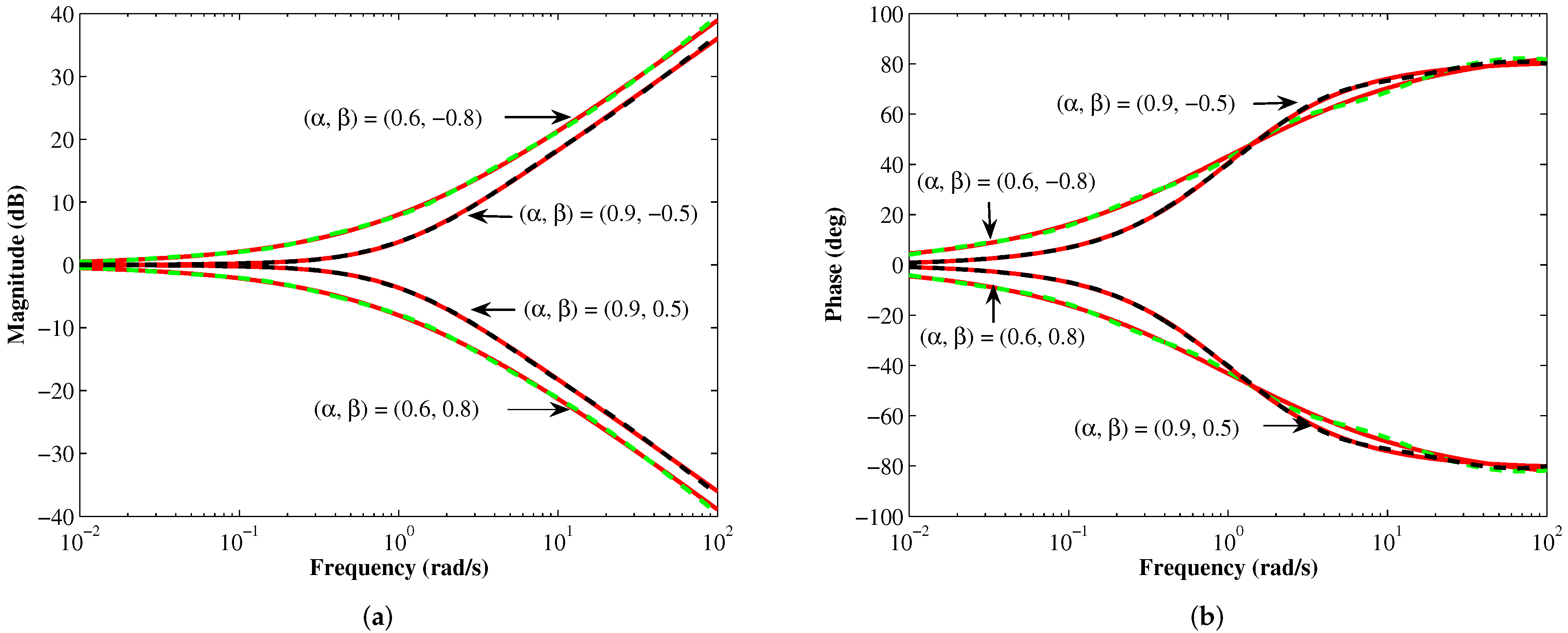
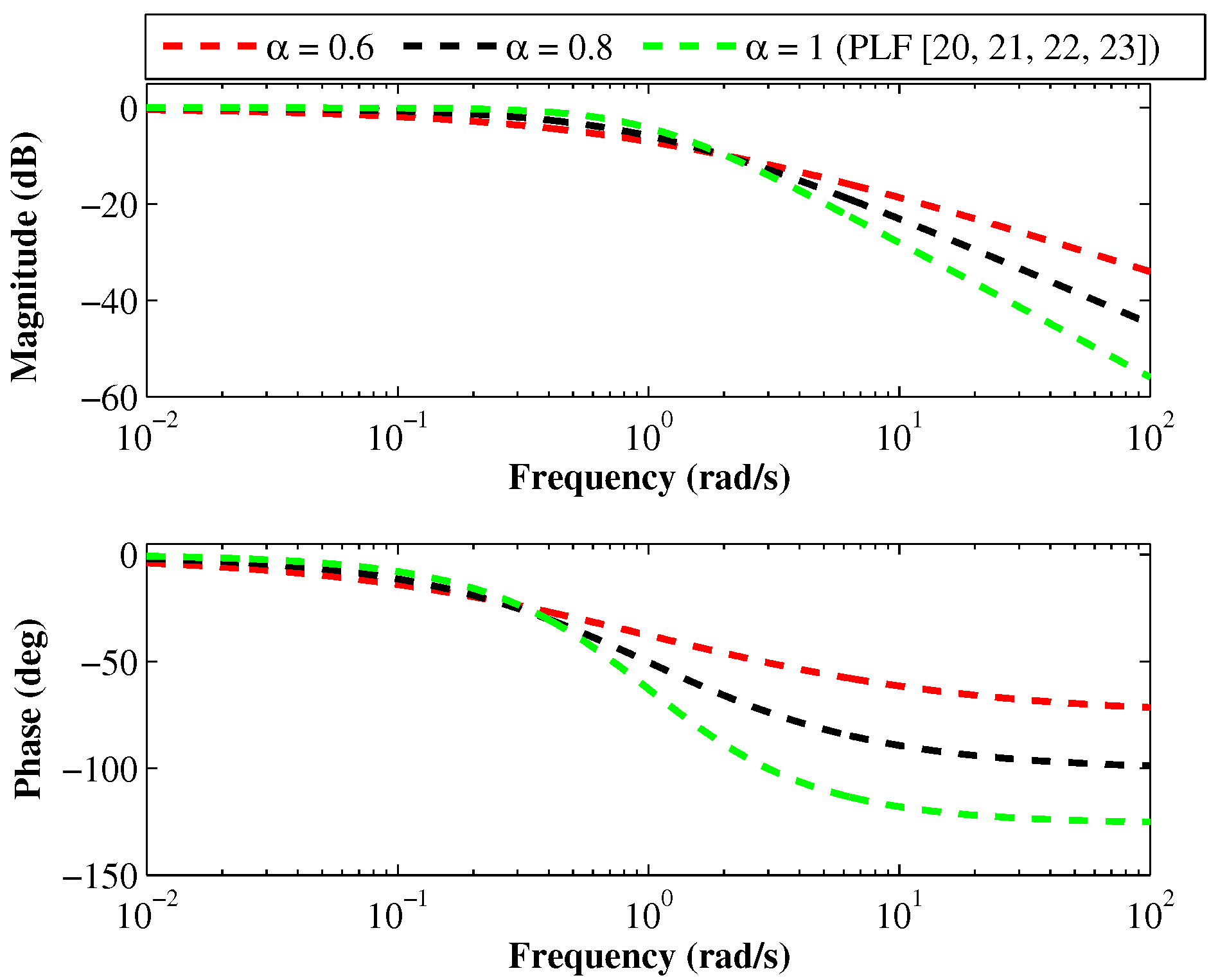
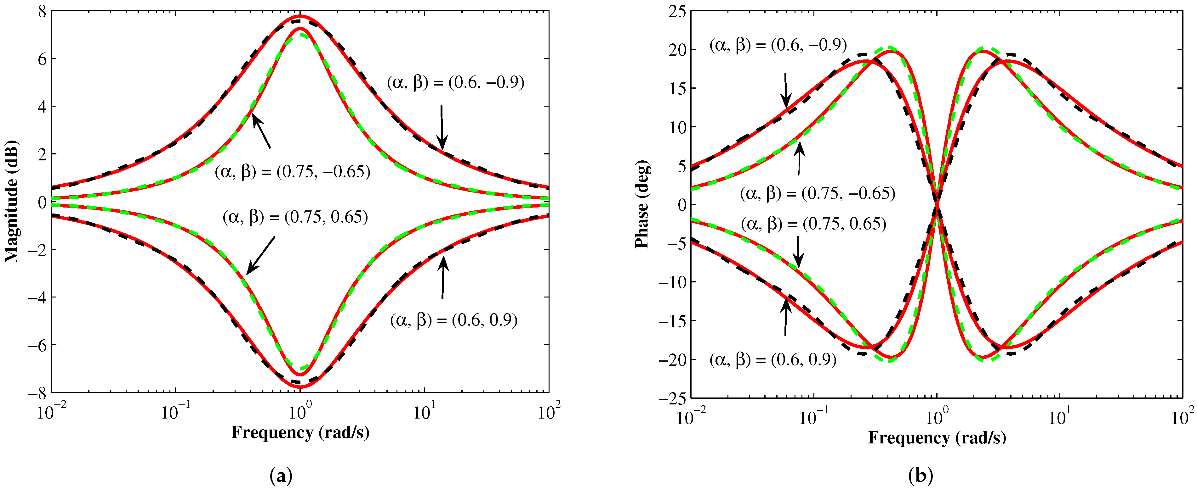
Figure 1.
Magnitude and phase responses of the theoretical FLPF for different values of with .
Figure 1.
Magnitude and phase responses of the theoretical FLPF for different values of with .
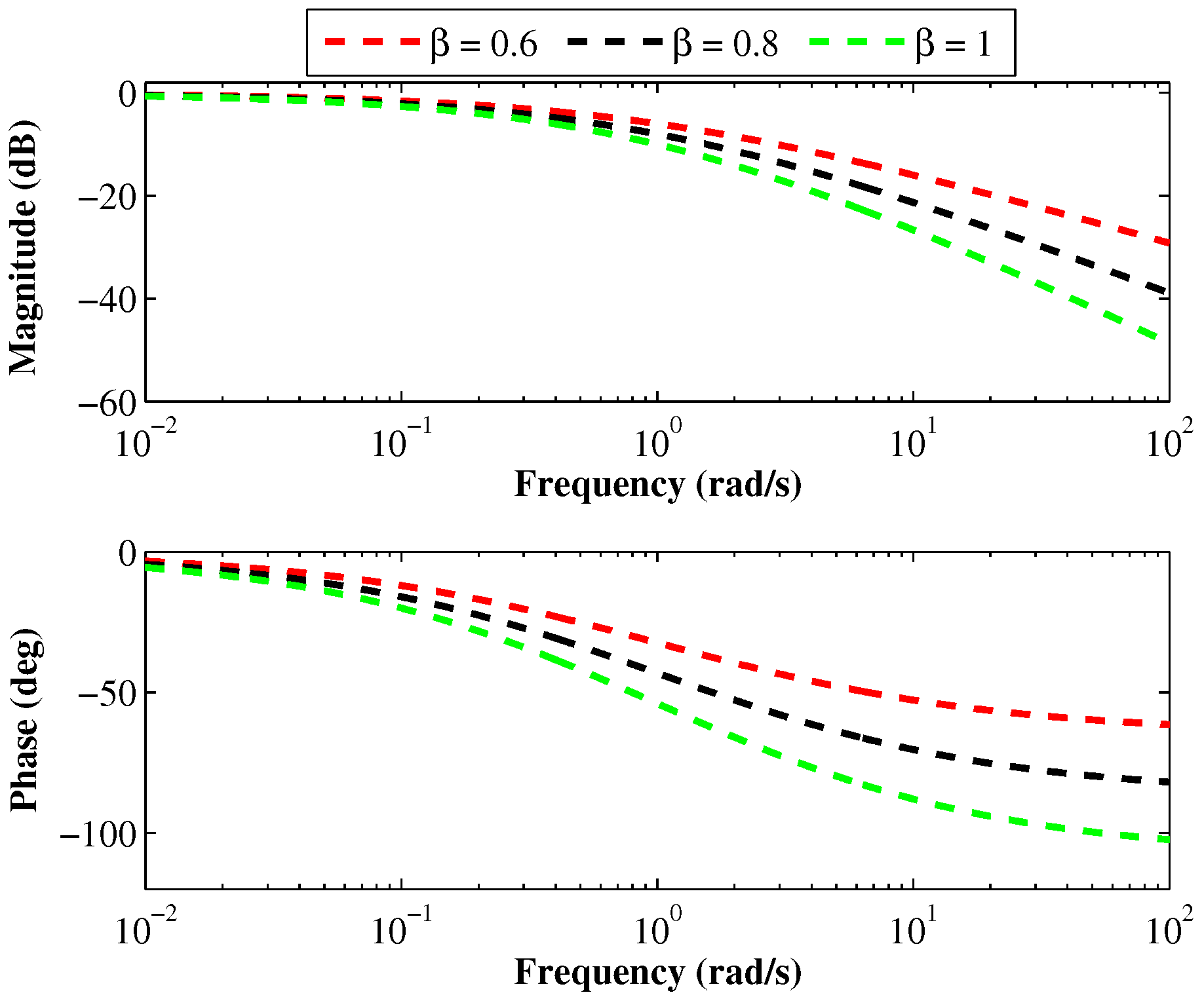
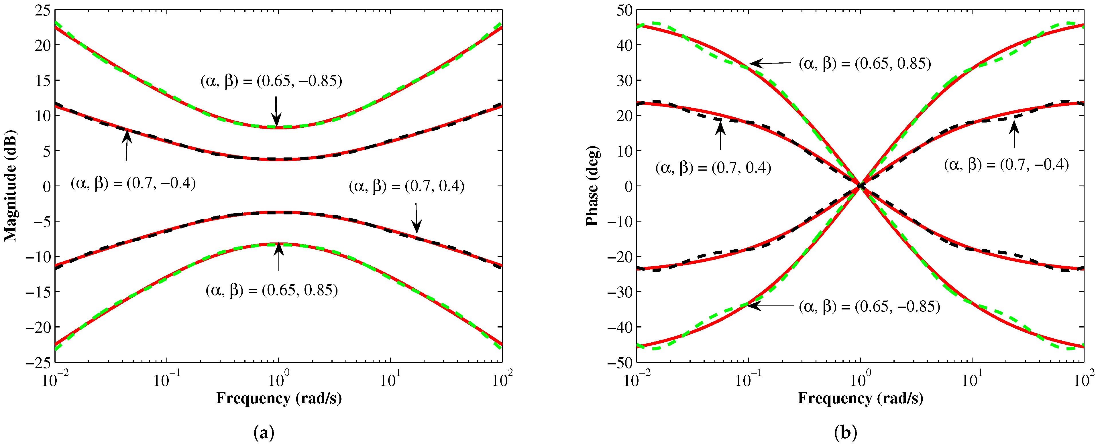
Figure 2.
Magnitude and phase responses of the theoretical FLPF for different values of with .
Figure 2.
Magnitude and phase responses of the theoretical FLPF for different values of with .
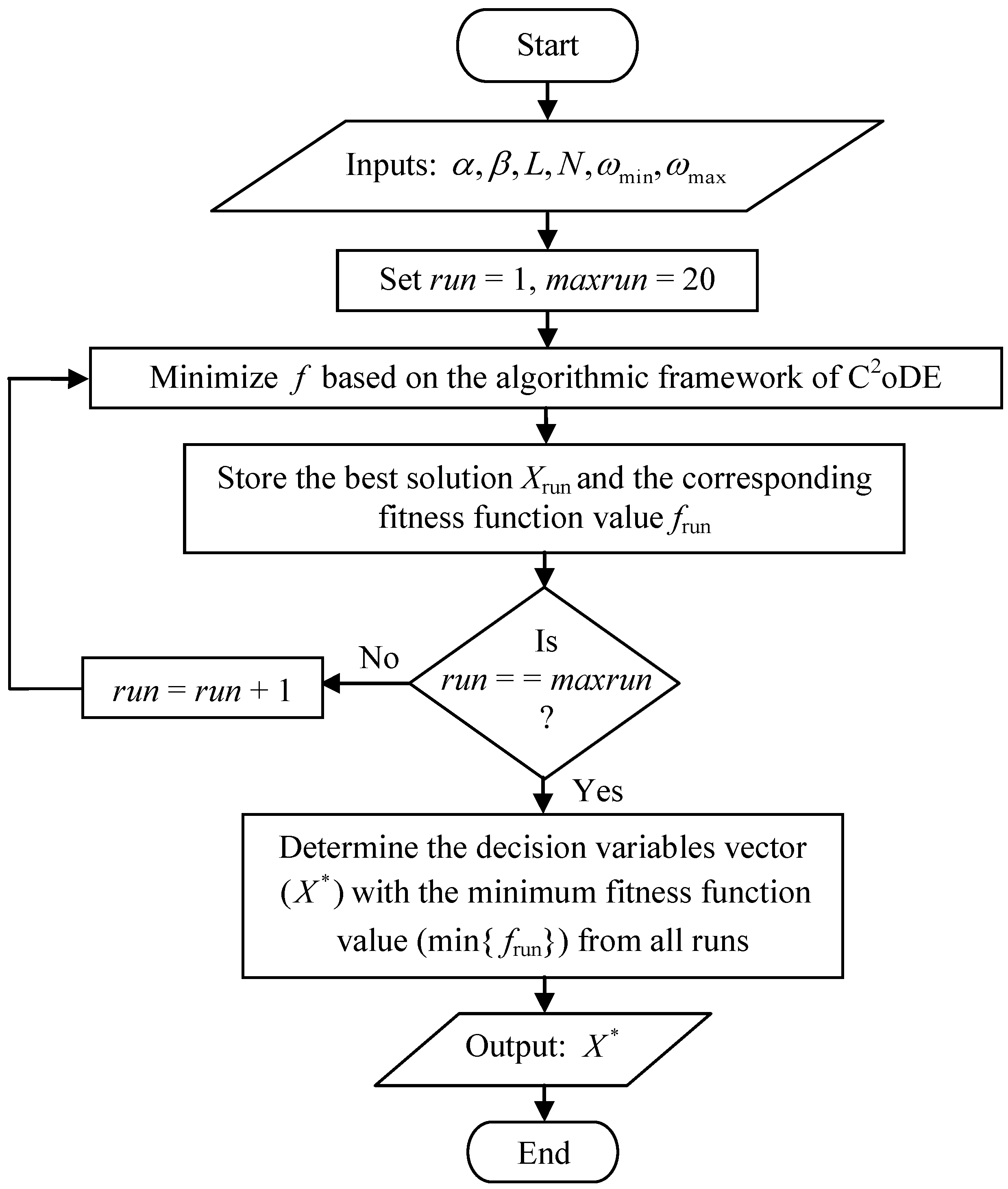
Figure 3.
Flowchart of the proposed filter design technique.
Figure 3.
Flowchart of the proposed filter design technique.
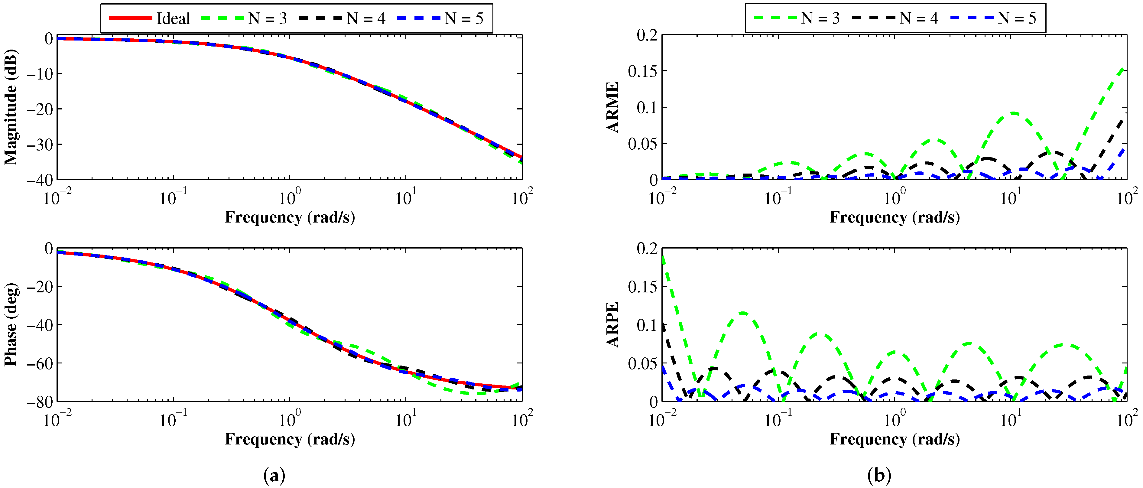
Figure 4.
(a) Magnitude, phase and (b) ARME, ARPE responses of the proposed FLPF (, ) for different values of N.
Figure 4.
(a) Magnitude, phase and (b) ARME, ARPE responses of the proposed FLPF (, ) for different values of N.
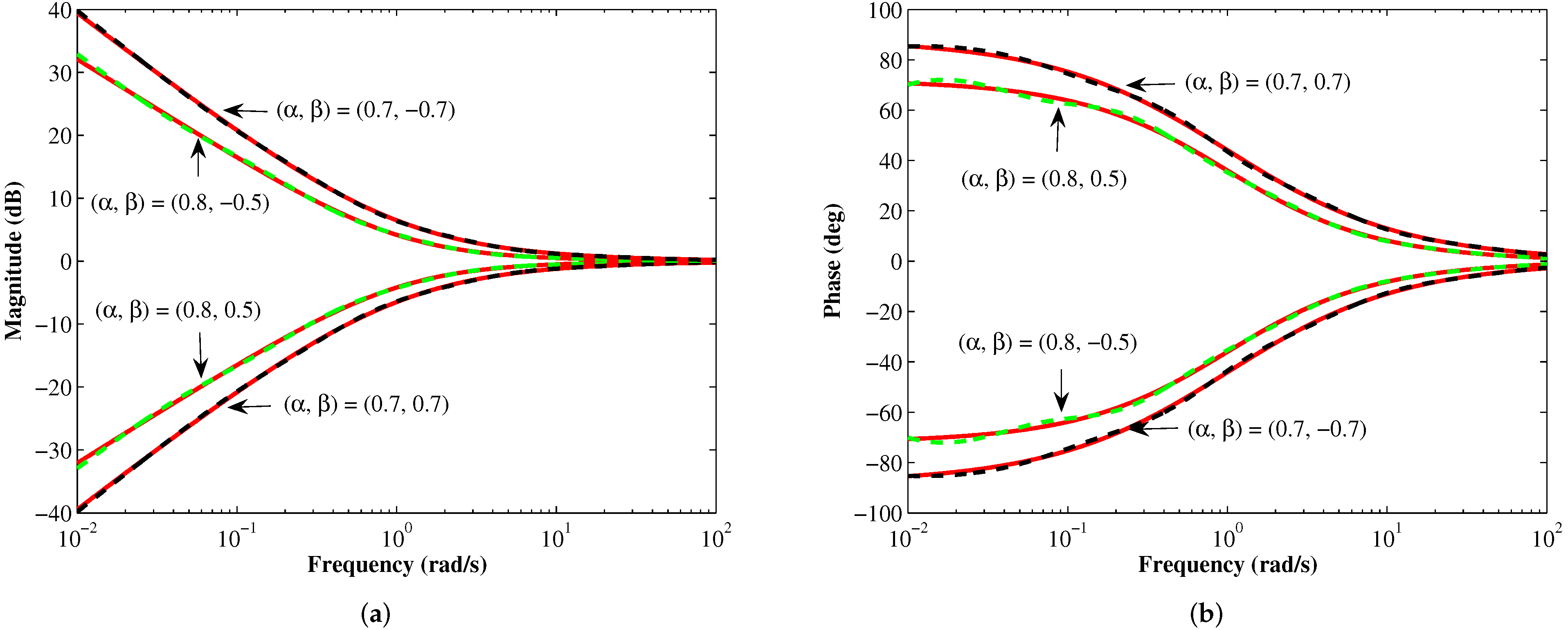
Figure 5.
(a) Magnitude and (b) phase responses of the proposed FLPFs and FILPFs for . The theoretical response is shown in solid red.
Figure 5.
(a) Magnitude and (b) phase responses of the proposed FLPFs and FILPFs for . The theoretical response is shown in solid red.
Figure 6.
(a) Magnitude and (b) phase responses of the proposed FHPFs and FIHPFs for . The theoretical response is shown in solid red.
Figure 6.
(a) Magnitude and (b) phase responses of the proposed FHPFs and FIHPFs for . The theoretical response is shown in solid red.
Figure 7.
(a) Magnitude and (b) phase responses of the proposed FBPFs and FIBPFs for . The theoretical response is shown in solid red.
Figure 7.
(a) Magnitude and (b) phase responses of the proposed FBPFs and FIBPFs for . The theoretical response is shown in solid red.
Figure 8.
(a) Magnitude and (b) phase responses of the proposed FBSFs and FIBSFs for . The theoretical response is shown in solid red.
Figure 8.
(a) Magnitude and (b) phase responses of the proposed FBSFs and FIBSFs for . The theoretical response is shown in solid red.
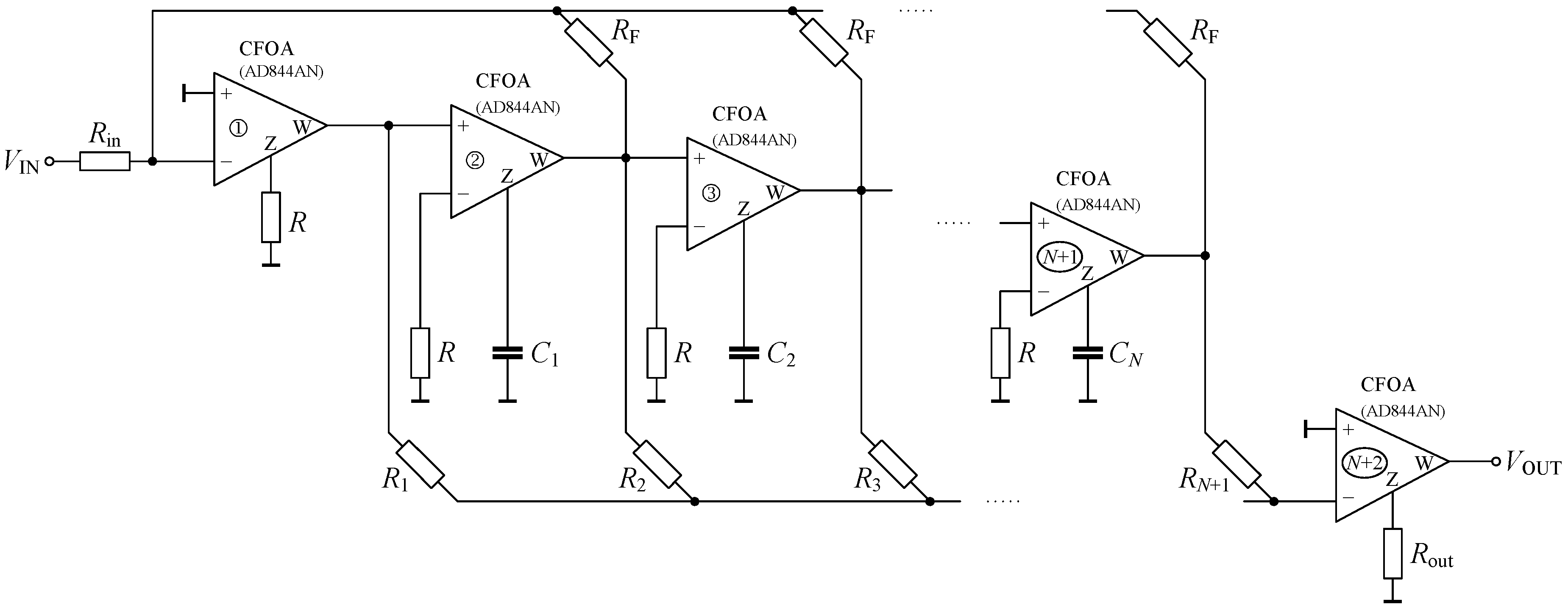
Figure 9.
CFOA-based circuit to realize the proposed filters.
Figure 9.
CFOA-based circuit to realize the proposed filters.
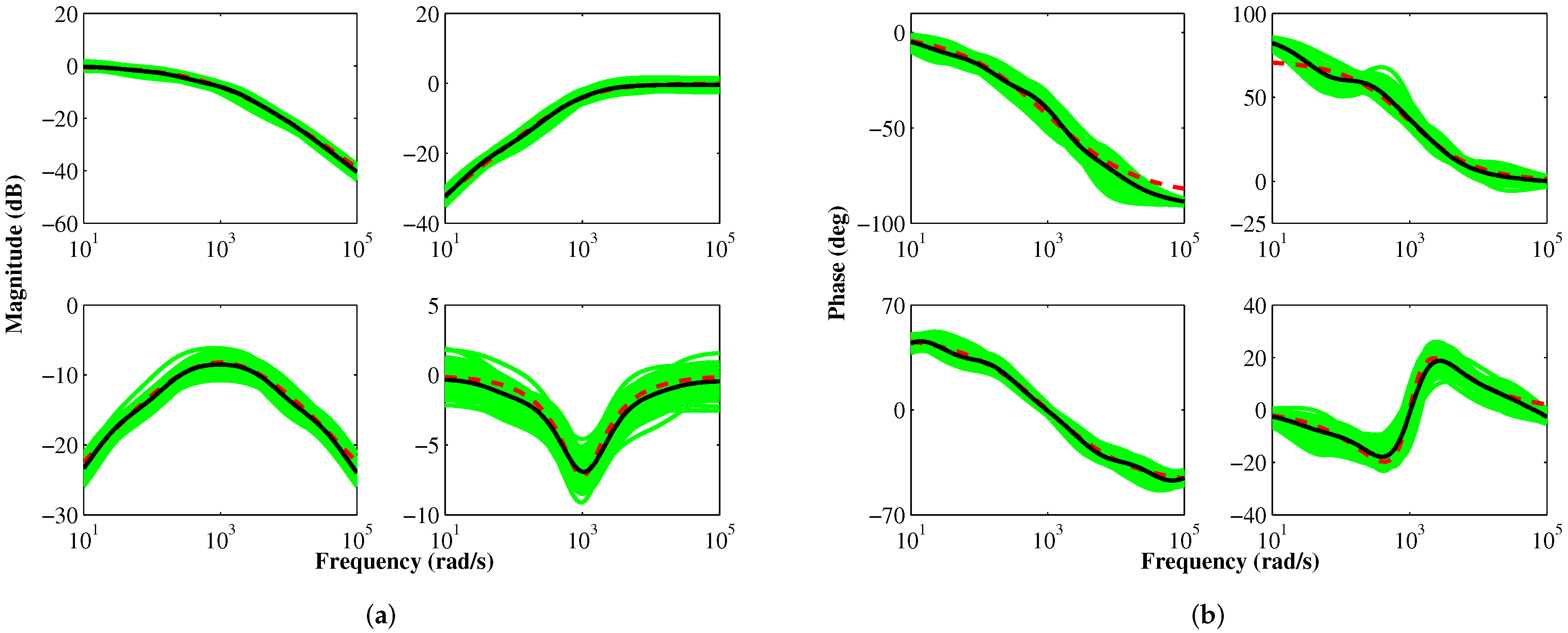
Figure 10.
SPICE simulated (a) magnitude and (b) phase responses of the proposed FLPF, FHPF, FBPF, and FBSF. [Note: Theoretical responses are shown in dashed red; responses based on nominal values of components are shown in solid black; Monte-Carlo simulation-based responses are shown in green].
Figure 10.
SPICE simulated (a) magnitude and (b) phase responses of the proposed FLPF, FHPF, FBPF, and FBSF. [Note: Theoretical responses are shown in dashed red; responses based on nominal values of components are shown in solid black; Monte-Carlo simulation-based responses are shown in green].
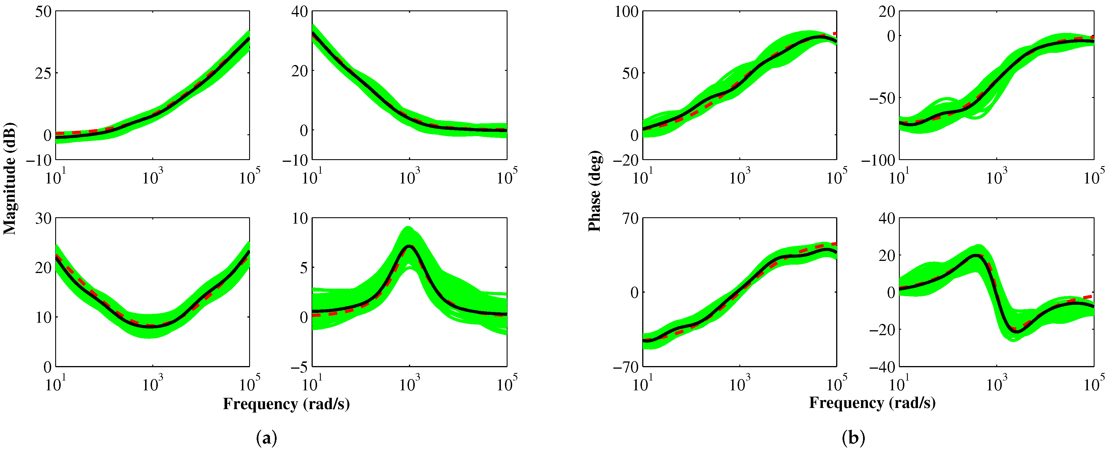
Figure 11.
SPICE simulated (a) magnitude and (b) phase responses of the proposed FILPF, FIHPF, FIBPF, and FIBSF. [Note: Theoretical responses are shown in dashed red; responses based on nominal values of components are shown in solid black; Monte-Carlo simulation-based responses are shown in green].
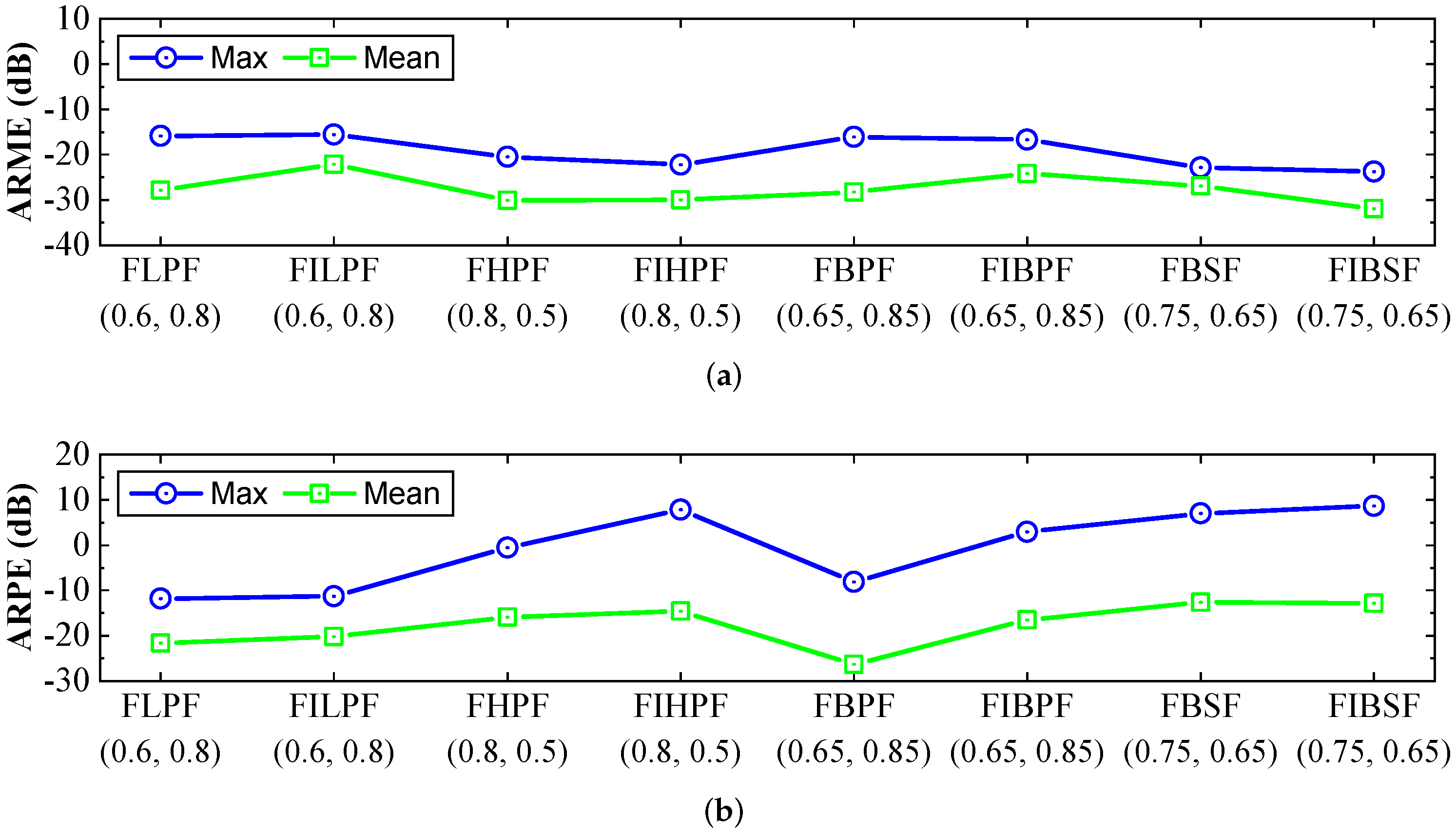
Figure 12.
Broken line plots of the (a) ARME and (b) ARPE responses for the SPICE simulated proposed FLPF, FHPF, FBPF, FBSF, and their inverse counterparts realized using the nominal values of components.
Figure 12.
Broken line plots of the (a) ARME and (b) ARPE responses for the SPICE simulated proposed FLPF, FHPF, FBPF, FBSF, and their inverse counterparts realized using the nominal values of components.
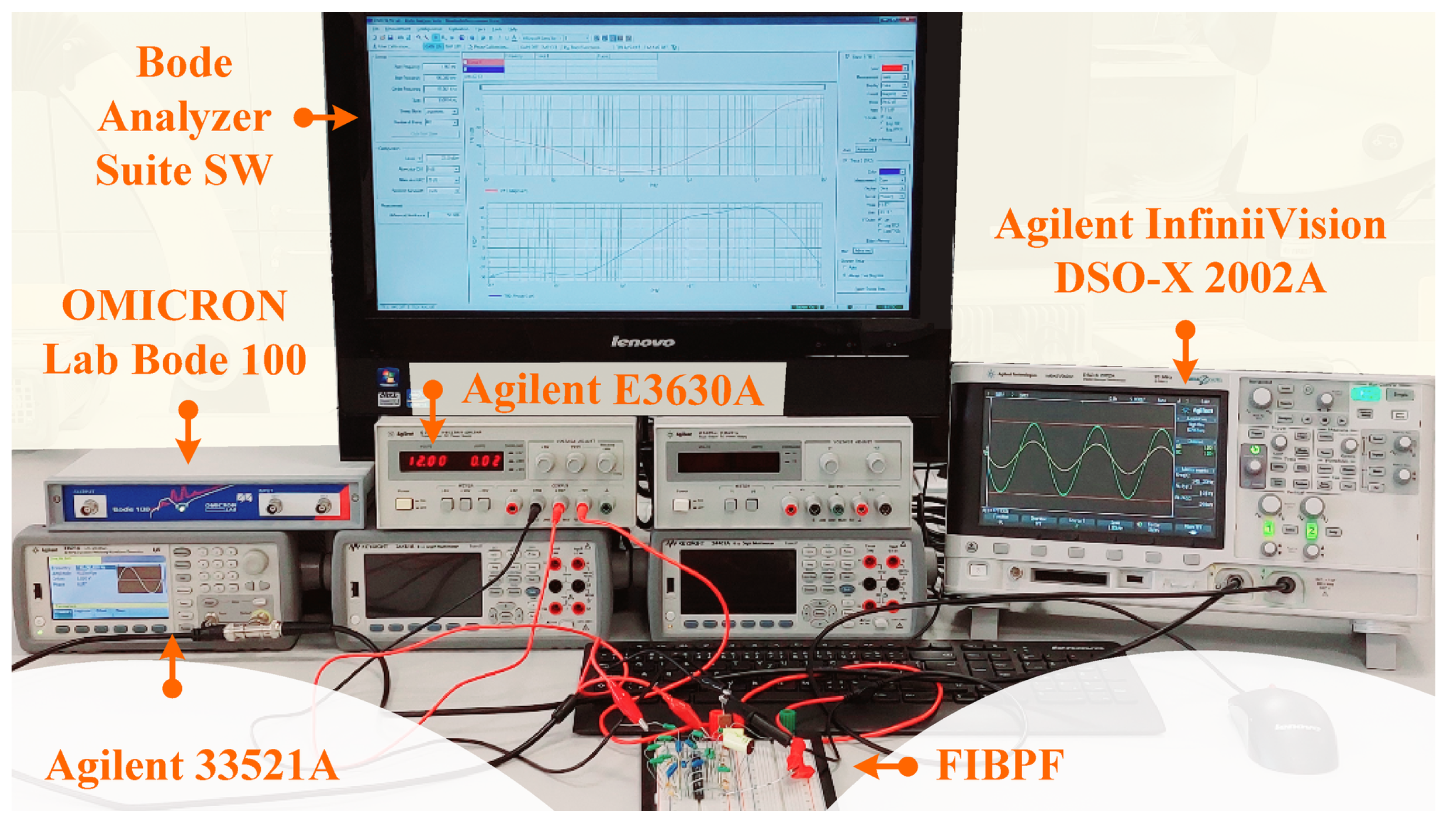
Figure 13.
Photograph of the experimental set-up.
Figure 13.
Photograph of the experimental set-up.
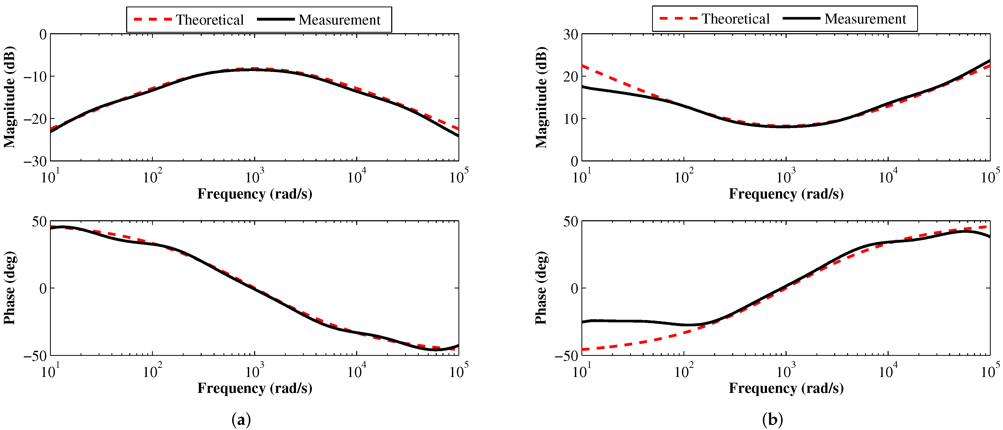
Figure 14.
Magnitude and phase responses of the proposed (a) FBPF and (b) FIBPF based on experimental measurements.
Figure 14.
Magnitude and phase responses of the proposed (a) FBPF and (b) FIBPF based on experimental measurements.
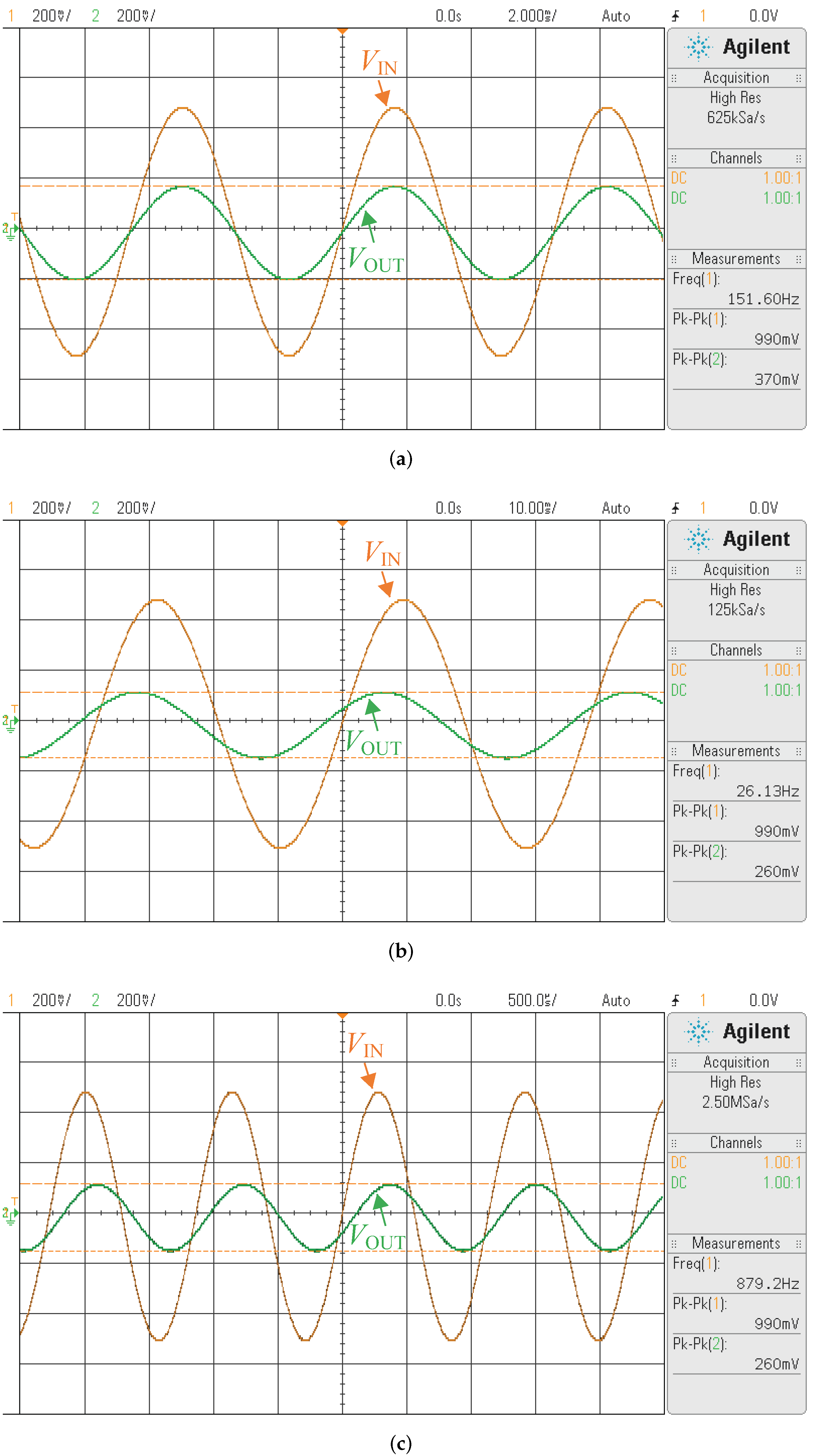
Figure 15.
Time-domain input-output waveforms observed in oscilloscope for the proposed FBPF with an input frequency of (a) rad/s, (b) rad/s, and (c) krad/s.
Figure 15.
Time-domain input-output waveforms observed in oscilloscope for the proposed FBPF with an input frequency of (a) rad/s, (b) rad/s, and (c) krad/s.
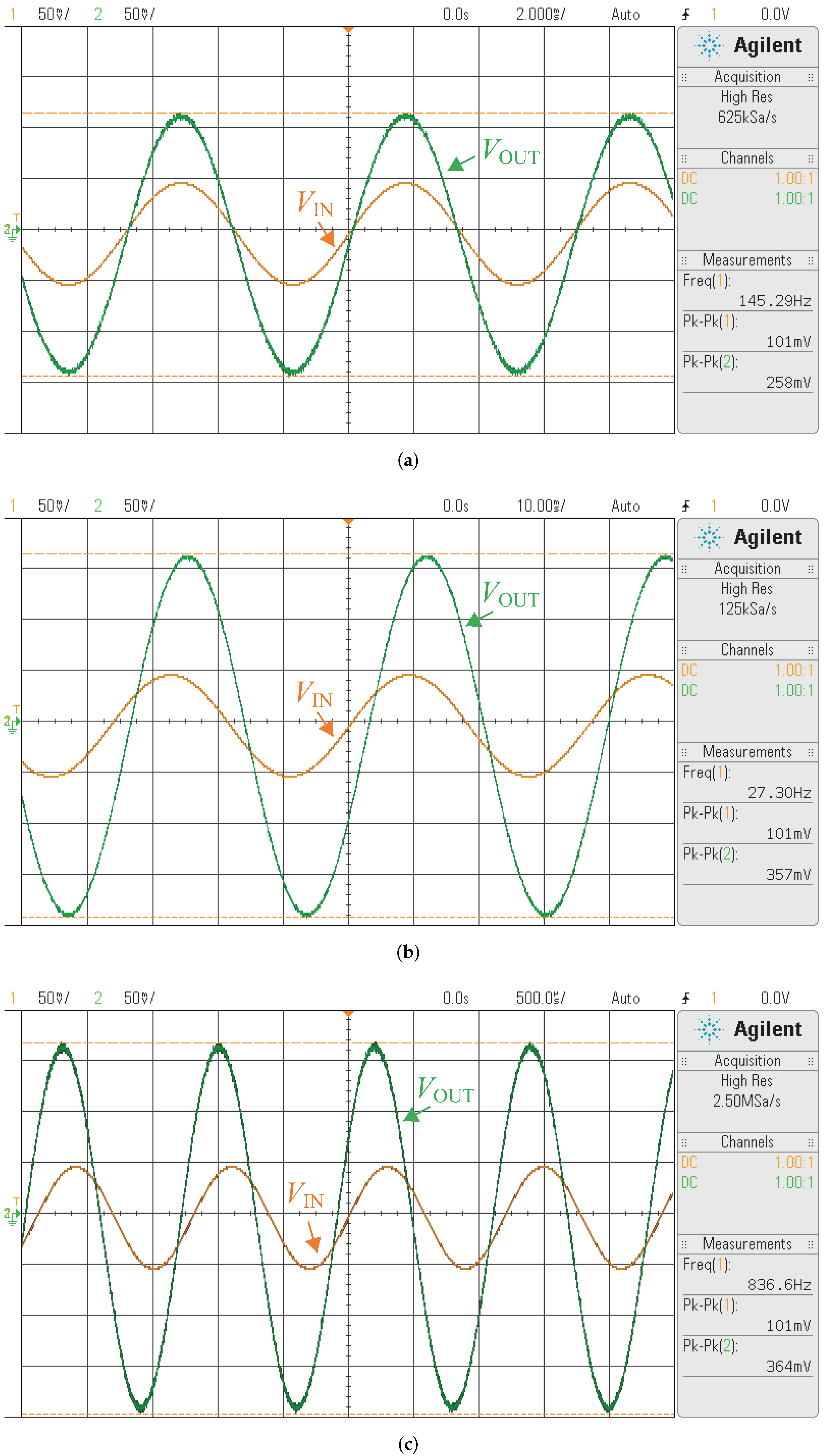
Figure 16.
Time-domain input-output waveforms observed in oscilloscope for the proposed FIBPF with an input frequency of (a) rad/s, (b) rad/s, and (c) krad/s.
Figure 16.
Time-domain input-output waveforms observed in oscilloscope for the proposed FIBPF with an input frequency of (a) rad/s, (b) rad/s, and (c) krad/s.
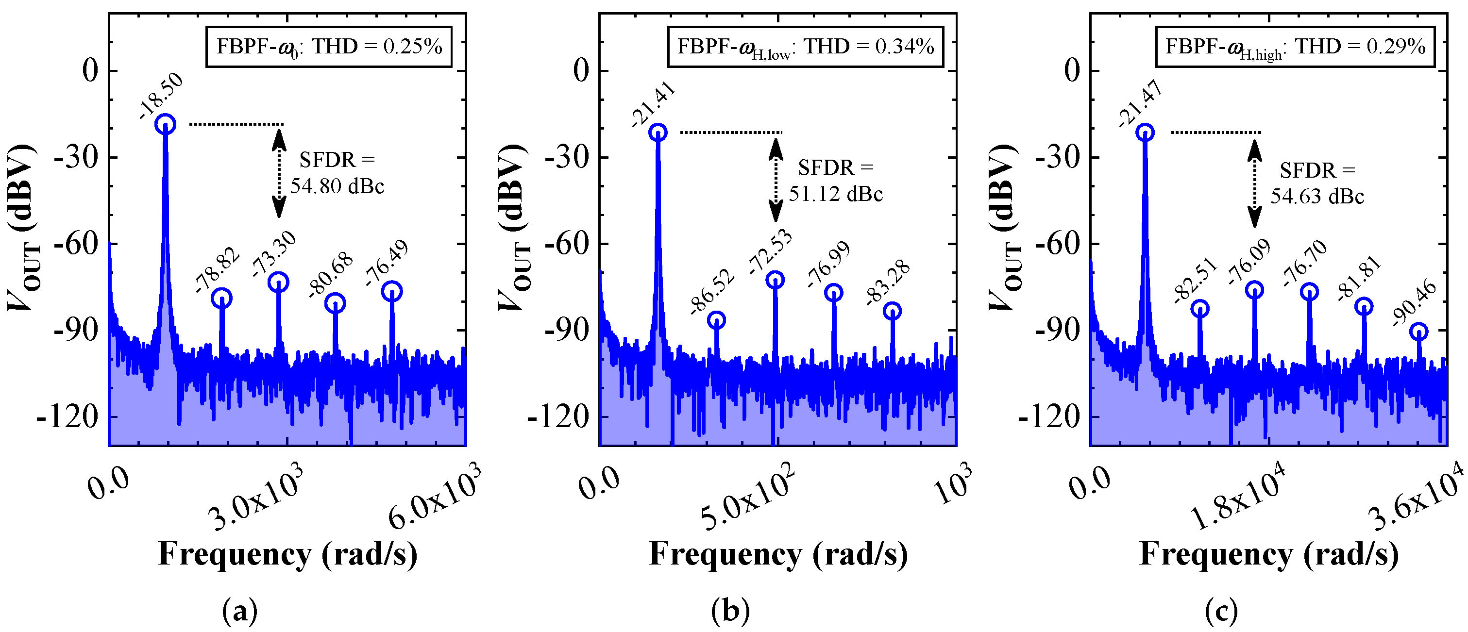
Figure 17.
Experimentally obtained Fourier spectrums of the proposed FBPF at frequency of (a) rad/s, (b) rad/s, and (c) krad/s.
Figure 17.
Experimentally obtained Fourier spectrums of the proposed FBPF at frequency of (a) rad/s, (b) rad/s, and (c) krad/s.
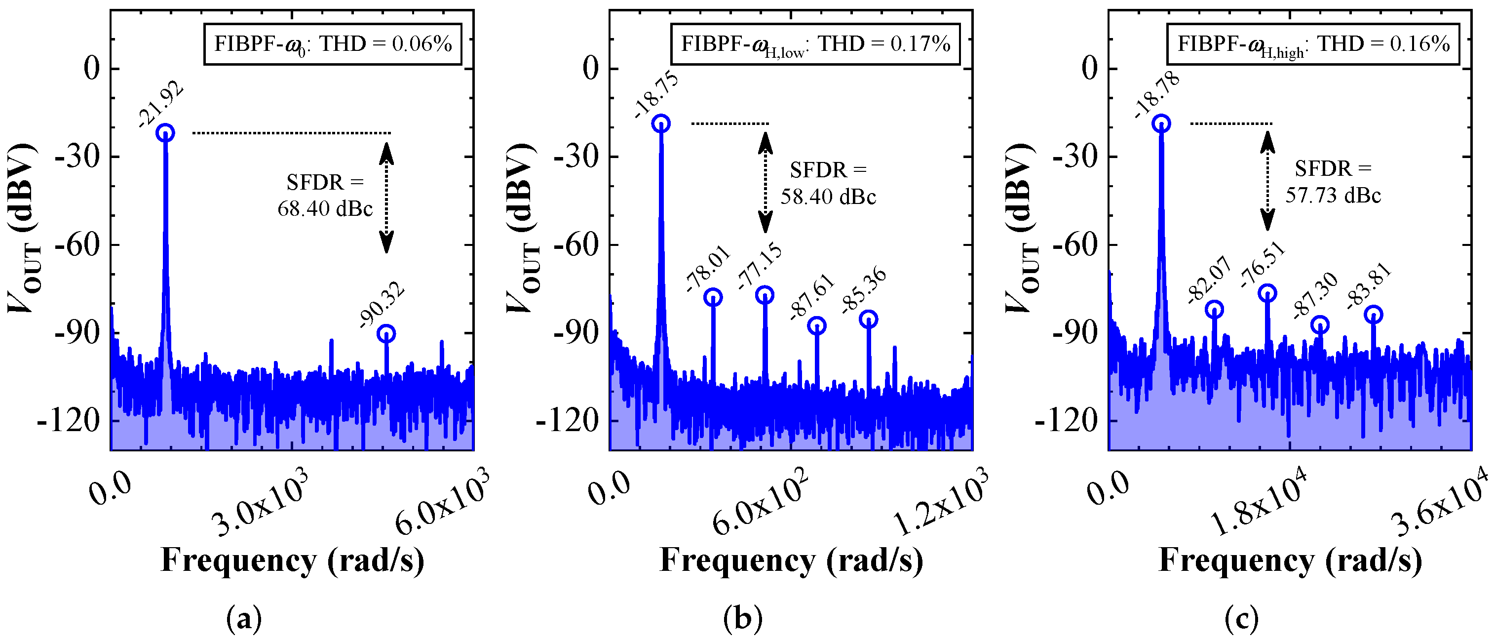
Figure 18.
Experimentally obtained Fourier spectrums of the proposed FIBPF at frequency of (a) rad/s, (b) rad/s, and (c) krad/s.
Figure 18.
Experimentally obtained Fourier spectrums of the proposed FIBPF at frequency of (a) rad/s, (b) rad/s, and (c) krad/s.
Table 1.
Transfer function, magnitude, and phase of the proposed theoretical filters.
Table 1.
Transfer function, magnitude, and phase of the proposed theoretical filters.
| Filter Type | Transfer Function | Parameter | Expression |
|---|
| Low-pass | | Magnitude | |
| Phase | |
| High-pass | | Magnitude | |
| Phase | |
| Band-pass | | Magnitude | |
| Phase | |
| Band-stop | | Magnitude | |
| Phase | |
Table 2.
Optimal coefficients of the proposed FLPFs for different values of , and N.
Table 2.
Optimal coefficients of the proposed FLPFs for different values of , and N.
| | N | [a a … a] | [bb … b] |
|---|
| 0.6 | 0.6 | 3 | 0.0142 2.5299 6.6189 0.4942 | 11.4218 9.2670 0.5131 |
| 4 | 0.0114 3.0287 25.5717 13.7481 0.4771 | 24.2389 55.7542 16.8974 0.4922 |
| 5 | 0.0092 3.4666 61.4831 110.5999 22.6230 0.4607 | 41.6920 208.3549 178.6875 26.2131 0.4730 |
| 0.6 | 0.8 | 3 | 0.0013 0.9827 1.6323 0.0935 | 4.7579 2.3646 0.0980 |
| 4 | 0.0010 1.0608 6.4002 2.5499 0.0741 | 11.0810 15.1524 3.2481 0.0770 |
| 5 | 0.0008 1.1094 15.6780 21.3117 3.5163 0.0625 | 21.2276 62.7773 37.1129 4.2024 0.0646 |
| 0.7 | 0.6 | 3 | 0.0051 1.6591 4.5010 0.3897 | 7.7235 5.9418 0.3968 |
| 4 | 0.0041 1.8637 16.5030 9.4477 0.3705 | 17.7793 34.5354 11.0523 0.3761 |
| 5 | 0.0031 2.0251 38.1221 70.6279 15.5349 0.3518 | 32.3963 132.0535 107.9572 17.2623 0.3562 |
| 0.9 | 0.5 | 3 | 0.0021 1.4230 6.3582 0.9979 | 7.7812 7.7812 1.0000 |
| 4 | 0.0018 1.5155 18.6555 16.4228 0.9982 | 17.9383 37.3110 17.9383 1.0000 |
| 5 | 0.0014 1.5881 38.2769 97.7768 30.9821 0.9986 | 32.5702 136.0537 136.0537 32.5702 1.0000 |
Table 3.
Performance indices of the designed FLPFs for different values of N.
Table 3.
Performance indices of the designed FLPFs for different values of N.
| | N | ARME (dB) | ARPE (dB) | (dB) | (deg) | (rad/s) | (rad/s) |
|---|
| Max | Mean | Max | Mean |
|---|
| 0.6 | 0.6 | 3 | −15.00 | −26.51 | −13.04 | −21.96 | −5.937 | −35.72 | 1.0210 | 0.7918 |
| 4 | −19.00 | −34.16 | −18.72 | −29.74 | −6.054 | −30.85 | 0.9886 | 1.1610 |
| 5 | −24.33 | −41.81 | −26.29 | −37.09 | −6.013 | −32.99 | 1.0030 | 0.9484 |
| 0.6 | 0.8 | 3 | −17.93 | −28.88 | −15.09 | −25.73 | −8.348 | −45.08 | 0.9380 | 0.8406 |
| 4 | −23.49 | −36.76 | −21.59 | −33.59 | −7.887 | −42.35 | 1.0380 | 1.0530 |
| 5 | −29.09 | −44.52 | −29.88 | −41.41 | −8.092 | −43.52 | 0.9867 | 0.9768 |
| 0.7 | 0.6 | 3 | −15.98 | −28.08 | −14.46 | −24.99 | −5.539 | −40.24 | 1.0060 | 0.8658 |
| 4 | −20.75 | −36.53 | −19.84 | −32.82 | −5.569 | −36.66 | 0.9995 | 1.0820 |
| 5 | −26.28 | −44.21 | −26.75 | −40.12 | −5.564 | −38.24 | 0.9999 | 0.9723 |
| 0.9 | 0.5 | 3 | −20.25 | −35.53 | −20.13 | −31.91 | −3.555 | −41.18 | 1.0220 | 0.9725 |
| 4 | −25.36 | −43.34 | −25.31 | −39.78 | −3.685 | −40.19 | 0.9895 | 1.0150 |
| 5 | −31.21 | −51.13 | −31.51 | −47.24 | −3.628 | −40.63 | 1.0040 | 0.9949 |
Table 4.
Optimal coefficients of the proposed FHPFs for different values of , and N.
Table 4.
Optimal coefficients of the proposed FHPFs for different values of , and N.
| | N | [a a … a] | [bb … b] |
|---|
| 0.8 | 0.5 | 3 | 0.9932 7.8453 2.0344 0.0068 | 9.8797 9.8797 1.0000 |
| 4 | 0.9944 19.1491 24.7984 2.2881 0.0056 | 21.4372 49.5967 21.4372 1.0000 |
| 5 | 0.9956 35.4326 126.2330 54.3189 2.5130 0.0044 | 37.9456 180.5519 180.5519 37.9456 1.0000 |
| 0.7 | 0.7 | 3 | 0.9806 14.6603 8.9401 0.0051 | 19.1412 35.6366 9.0971 |
| 4 | 0.9838 29.7348 70.3640 12.4674 0.0062 | 34.9174 142.9660 108.5833 12.1205 |
| 5 | 0.9867 49.5131 277.8629 204.4321 15.4272 0.0055 | 55.3552 426.0090 692.3231 257.6597 14.6294 |
Table 5.
Performance indices of the designed FHPFs for different values of N.
Table 5.
Performance indices of the designed FHPFs for different values of N.
| | N | ARME (dB) | ARPE (dB) | (dB) | (deg) | (rad/s) | (rad/s) |
|---|
| Max | Mean | Max | Mean |
|---|
| 0.8 | 0.5 | 3 | −16.36 | −30.39 | −15.52 | −26.32 | −4.016 | 37.42 | 0.9607 | 1.0750 |
| 4 | −20.88 | −38.15 | −20.54 | −34.09 | −4.253 | 35.31 | 1.0240 | 0.9563 |
| 5 | −26.75 | −45.88 | −27.31 | −41.43 | −4.150 | 36.25 | 0.9931 | 1.0150 |
| 0.7 | 0.7 | 3 | −21.94 | −32.77 | −16.23 | −28.43 | −6.697 | 45.32 | 1.0450 | 1.0890 |
| 4 | −27.92 | −40.83 | −21.92 | −36.56 | −6.394 | 43.54 | 0.9772 | 0.9723 |
| 5 | −33.70 | −48.61 | −29.96 | −44.31 | −6.527 | 44.29 | 1.0100 | 1.0130 |
Table 6.
Optimal coefficients of the proposed FBPFs for different values of , and N.
Table 6.
Optimal coefficients of the proposed FBPFs for different values of , and N.
| | N | [a a … a] | [bb … b] |
|---|
| 0.65 | 0.85 | 3 | 0.0455 4.3916 4.3916 0.0455 | 14.0152 14.0152 1.0000 |
| 4 | 0.0340 6.8775 71.8572 6.8775 0.0340 | 43.2076 189.9142 43.2076 1.0000 |
| 5 | 0.0324 7.2641 93.9189 93.9189 7.2641 0.0324 | 49.2315 278.9397 278.9397 49.2315 1.0000 |
| 6 | 0.0250 9.5746 317.2759 1481.1000 | 95.0273 1388.1000 3966.1000 1388.1000 |
| | 317.2759 9.5746 0.0250 | 95.0273 1.0000 |
| 7 | 0.0242 9.9057 365.7414 2150.5001 2150.5001 | 102.9711 1704.5000 6397.6000 6397.6000 |
| | 365.7414 9.9057 0.0242 | 1704.5000 102.9711 1.0000 |
| 0.7 | 0.4 | 3 | 0.2225 12.8293 12.8293 0.2225 | 22.5980 22.5980 1.0000 |
| 4 | 0.1890 24.6291 220.2190 24.6291 0.1890 | 62.3458 342.9724 62.3458 1.0000 |
| 5 | 0.1853 26.4413 291.1292 291.1292 26.4413 0.1853 | 69.4012 483.2816 483.2816 69.4012 1.0000 |
| 6 | 0.1622 40.1465 1131.1000 4864.2000 | 128.0391 2342.3000 7601.1000 2342.3000 |
| | 1131.1000 40.1465 0.1622 | 128.0391 1.0000 |
| 7 | 0.1595 42.2490 1326.8000 7221.5000 7221.5000 | 137.9077 2840.7000 11974.0000 11974.0000 |
| | 1326.8000 42.2490 0.1595 | 2840.7000 137.9077 1.0000 |
Table 7.
Performance indices of the designed FBPFs for different values of N.
Table 7.
Performance indices of the designed FBPFs for different values of N.
| | N | ARME (dB) | ARPE (dB) | BW (rad/s) | (dB) | (deg) |
|---|
| Max | Mean | Max | Mean |
|---|
| 0.65 | 0.85 | 3 | −14.76 | −19.32 | −4.86 | −11.75 | 13.205 | −9.527 | −0.0035 |
| 4 | −21.68 | −34.50 | −17.52 | −27.36 | 6.073 | −8.358 | −0.0070 |
| 5 | −23.21 | −34.64 | −15.06 | −25.71 | 6.417 | −8.433 | −0.0067 |
| 6 | −36.08 | −49.89 | −30.04 | −41.07 | 5.835 | −8.242 | −0.0079 |
| 7 | −38.61 | −49.95 | −27.18 | −39.68 | 5.840 | −8.255 | −0.0078 |
| 0.7 | 0.4 | 3 | −18.03 | −22.91 | −3.53 | −9.83 | 25.571 | −4.676 | −0.0015 |
| 4 | −26.72 | −38.04 | −15.16 | −24.90 | 11.947 | −3.812 | −0.0037 |
| 5 | −28.00 | −37.99 | −12.91 | −23.35 | 12.380 | −3.868 | −0.0035 |
| 6 | −41.30 | −53.22 | −27.44 | −38.60 | 12.601 | −3.724 | −0.0043 |
| 7 | −43.93 | −53.12 | −24.66 | −37.14 | 12.621 | −3.734 | −0.0042 |
Table 8.
Optimal coefficients of the proposed FBSFs for different values of , and N.
Table 8.
Optimal coefficients of the proposed FBSFs for different values of , and N.
| | N | [a a … a] | [bb … b] |
|---|
| 0.75 | 0.65 | 4 | 0.9888 21.8400 31.5924 21.8400 0.9888 | 25.4992 68.2322 25.4992 1.0000 |
| 6 | 0.9926 58.0809 430.8486 556.5188 | 62.5308 575.3021 1133.4000 |
| | 430.8486 58.0809 0.9926 | 575.3021 62.5308 1.0000 |
| 0.6 | 0.9 | 4 | 0.9562 31.9360 76.3241 31.9360 0.9562 | 41.7298 179.7455 41.7298 1.0000 |
| 6 | 0.9683 77.7410 845.4961 1556.4000 | 90.9584 1287.8000 3595.6000 |
| | 845.4961 77.7410 0.9683 | 1287.8000 90.9584 1.0000 |
Table 9.
Performance indices of the designed FBSFs for different values of N.
Table 9.
Performance indices of the designed FBSFs for different values of N.
| | N | ARME (dB) | ARPE (dB) | BW (rad/s) | (dB) | (deg) |
|---|
| Max | Mean | Max | Mean |
|---|
| 0.75 | 0.65 | 4 | −30.30 | −43.99 | −15.30 | −28.03 | 2.018 | −6.991 | 0.0186 |
| 6 | −43.71 | −57.38 | −25.92 | −41.60 | 1.793 | −7.196 | 0.0213 |
| 0.6 | 0.9 | 4 | −32.43 | −41.32 | −15.42 | −26.59 | 3.709 | −7.563 | 0.0102 |
| 6 | −48.63 | −56.24 | −28.33 | −41.33 | 3.350 | −7.736 | 0.0119 |
Table 10.
Coefficients of the proposed and reported filters for (NA: Not Applicable).
Table 10.
Coefficients of the proposed and reported filters for (NA: Not Applicable).
| Type | Reference | | [a a … a] | [bb … b] |
|---|
| FLPF | [20] | 0.7 | NA | NA |
| Present Work | 0.7 | 0.0848 11.9870 109.7033 87.4632 4.6137 | 43.3927 178.5692 96.6050 4.6538 |
| [20] | 1 | 0.02219 6.6070 171.1000 877.9000 999.4000 | 58.4100 578.6000 1477.0000 999.5000 |
| Present Work | 1 | 0.0197 7.1837 219.3990 1221.6000 1427.9000 | 70.6331 781.3135 2078.2000 1427.9000 |
| FHPF | [20] | 0.7 | NA | NA |
| Present Work | 0.7 | 0.9914 18.7939 23.5728 2.5757 0.0182 | 20.7582 38.3705 9.3241 0.2149 |
| [20] | 1 | 1.0000 0.8784 0.1712 0.006611 | 1.4780 0.5789 0.05844 0.001001 |
| Present Work | 1 | 1.0000 0.8556 0.1537 0.0050 | 1.4555 0.5472 0.0495 |
| FBPF | [20] | 0.7 | NA | NA |
| Present Work | 0.7 | 0.2927 32.2869 264.4314 32.2869 0.2927 | 64.3533 368.5848 64.3533 1.0000 |
| [20] | 1 | 0.2457 18.1300 97.4600 18.1300 0.2457 | 31.8200 99.4300 31.8200 1.0000 |
| Present Work | 1 | 0.1772 19.9502 149.8006 19.9502 0.1772 | 48.3274 189.2569 48.3274 1.0000 |
| FBSF | [20] | 0.7 | NA | NA |
| Present Work | 0.7 | 0.9919 23.9259 47.8177 23.9259 0.9919 | 25.9647 66.3058 25.9647 1.0000 |
| [20] | 1 | 0.9994 0.9467 2.0690 0.9467 0.9994 | 1.5350 2.2660 1.5350 1.0000 |
| Present Work | 1 | 0.9993 0.9207 2.0600 0.9207 0.9993 | 1.5080 2.2460 1.5080 1.0000 |
Table 11.
Error metrics comparison of the proposed filters with the reported literature for (NA: Not Applicable).
Table 11.
Error metrics comparison of the proposed filters with the reported literature for (NA: Not Applicable).
| Type | Reference | | ARME (dB) | ARPE (dB) |
|---|
| Max | Mean | Max | Mean |
|---|
| FLPF | [20] | 0.7 | NA | NA | NA | NA |
| Present Work | 0.7 | −21.59 | −38.13 | −16.17 | −28.87 |
| [20] | 1 | −23.82 | −50.60 | −33.80 | −51.11 |
| Present Work | 1 | −29.17 | −53.97 | −35.52 | −52.44 |
| FHPF | [20] | 0.7 | NA | NA | NA | NA |
| Present Work | 0.7 | −21.55 | −38.12 | −16.18 | −28.87 |
| [20] | 1 | −23.78 | −50.68 | −33.66 | −51.78 |
| Present Work | 1 | −27.73 | −52.98 | −35.18 | −52.54 |
| FBPF | [20] | 0.7 | NA | NA | NA | NA |
| Present Work | 0.7 | −28.15 | −40.40 | −15.21 | −25.08 |
| [20] | 1 | −11.50 | −13.19 | −11.69 | −26.76 |
| Present Work | 1 | −23.87 | −35.13 | −15.42 | −25.35 |
| FBSF | [20] | 0.7 | NA | NA | NA | NA |
| Present Work | 0.7 | −39.47 | −50.71 | −15.61 | −27.11 |
| [20] | 1 | −9.56 | −49.46 | −1.41 | −33.64 |
| Present Work | 1 | −11.63 | −48.97 | −1.64 | −33.12 |
Table 12.
Values of components to realize the proposed filters. [Note: Numbers in parenthesis represent ].
Table 12.
Values of components to realize the proposed filters. [Note: Numbers in parenthesis represent ].
| Component | FLPF | FILPF | FHPF | FIHPF | FBPF | FIBPF | FBSF | FIBSF |
|---|
| (0.6, 0.8) | (0.6, 0.8) | (0.8, 0.5) | (0.8, 0.5) | (0.65, 0.85) | (0.65, 0.85) | (0.75, 0.65) | (0.75, 0.65) |
|---|
| R (k | 10 | 100 | 10 | 100 | 7.5 | 100 | 75 | 100 |
| (k | 10 | 1 | 10 | 100 | 7.5 | 100 | 75 | 100 |
| (k | 10 | 100 | 10 | 11 | 7.5 | 10 | 75 | 110 |
| (k | 10 | 10 | 10 | 10 | 7.5 | 10 | 75 | 100 |
| (k | ∞ | 1 | 10 | 100 | 220 | 3.3 | 75 | 100 |
| (k | 100 | 1 | 11 | 91 | 47 | 16 | 91 | 82 |
| (k | 24 | 4.3 | 20 | 51 | 20 | 39 | 160 | 47 |
| (k | 13 | 8.2 | 91 | 11 | 47 | 16 | 91 | 82 |
| (k | 10 | 10 | ∞ | 0.56 | 220 | 3.3 | 75 | 100 |
| (nF) | 10 | 1 | 4.7 | 0.56 | 3.3 | 0.047 | 0.56 | 0.47 |
| (nF) | 68 | 1.8 | 47 | 8.2 | 33 | 1 | 4.7 | 6.8 |
| (nF) | 470 | 27 | 220 | 100 | 560 | 100 | 33 | 15 |
| (F) | 3.9 | 0.33 | 2.2 | 3.9 | 5.6 | 2.2 | 0.33 | 0.22 |
Table 13.
ARME and ARPE performances of the SPICE-simulated proposed filters based on nominal values of components.
Table 13.
ARME and ARPE performances of the SPICE-simulated proposed filters based on nominal values of components.
| Metric | Index | FLPF | FILPF | FHPF | FIHPF | FBPF | FIBPF | FBSF | FIBSF |
|---|
| (0.6, 0.8) | (0.6, 0.8) | (0.8, 0.5) | (0.8, 0.5) | (0.65, 0.85) | (0.65, 0.85) | (0.75, 0.65) | (0.75, 0.65) |
|---|
| ARME (dB) | Max | −15.84 | −15.52 | −20.50 | −22.19 | −16.05 | −16.66 | −22.85 | −23.72 |
| Mean | −27.80 | −22.10 | −30.05 | −29.94 | −28.24 | −24.11 | −26.94 | −31.91 |
| ARPE (dB) | Max | −11.77 | −11.32 | −0.56 | 7.88 | −8.07 | 2.90 | 6.97 | 8.67 |
| Mean | −21.61 | −20.20 | −15.92 | −14.56 | −26.31 | −16.47 | −12.57 | −12.87 |
Table 14.
Statistical indices about the magnitude/phase at the shift frequency of the designed filters based on 100 Monte-Carlo simulation runs.
Table 14.
Statistical indices about the magnitude/phase at the shift frequency of the designed filters based on 100 Monte-Carlo simulation runs.
| Parameter | Index | FLPF | FILPF | FHPF | FIHPF | FBPF | FIBPF | FBSF | FIBSF |
|---|
| @ 1 krad/s | (0.6, 0.8) | (0.6, 0.8) | (0.8, 0.5) | (0.8, 0.5) | (0.65, 0.85) | (0.65, 0.85) | (0.75, 0.65) | (0.75, 0.65) |
|---|
Magnitude
(dB) | Min | −10.56 | 5.60 | −5.98 | 1.68 | −10.75 | 5.99 | −9.10 | 4.95 |
| Max | −6.22 | 9.79 | −1.72 | 6.11 | −6.18 | 10.15 | −4.58 | 8.98 |
| Mean | −7.99 | 7.55 | −4.05 | 3.78 | −8.50 | 8.03 | −6.88 | 7.08 |
| SD | 0.932 | 0.921 | 0.972 | 0.962 | 0.898 | 0.851 | 0.902 | 0.850 |
| Ideal | −8.02 | 8.02 | −4.18 | 4.18 | −8.22 | 8.22 | −7.25 | 7.25 |
Phase
(deg) | Min | −52.42 | 34.16 | 31.03 | −51.45 | −4.19 | −4.02 | −14.24 | −11.79 |
| Max | −31.51 | 54.64 | 49.47 | −27.64 | 4.24 | 5.99 | 9.63 | 9.86 |
| Mean | −41.07 | 42.07 | 38.10 | −36.59 | −0.13 | 2.15 | −1.07 | −0.56 |
| SD | 4.154 | 3.875 | 4.287 | 4.587 | 1.875 | 1.747 | 4.393 | 4.692 |
| Ideal | −43.20 | 43.20 | 36.00 | −36.00 | 0.00 | 0.00 | 0.00 | 0.00 |


