Fractals Generated via Numerical Iteration Method

Abstract

In this research article, a modified algorithm for the generation of a fractal pattern resulting from the iteration of an algebraic function using the numerical iteration method is presented. This fractal pattern shows the dynamical behavior of the numerical iterations. A nonstandard convergence test of the displayable fractal pattern was applied.

1. Introduction

Benoit B. Mandelbrot [1] studied and extended the theory and graphic representations of iterated functions over the complex plane $ℂ$.

Let $f(z)$ be a complex-valued function. For a value of an initial complex number $z_0$ (usually 0) in the complex plane, $ℂ$, the function $f(z)$ is iterated using the iteration formula

$$z_k=f(z_{k-1}), k=1, 2, 3, \dots$$

Determine the dynamical behavior of $f(z)$ [2]. The sequence $z_0,z_1,z_2,\dots$ may converge or diverge depending on the coordinates of $z_0$ [3,4].

If quadratic complex valued-function $f(z)$ has zero-valued ${\alpha }_1 \mathrm{and} {\alpha }_2$ in $ℂ$ and $L$ is the perpendicular bisector of the line segment from ${\alpha }_1 \mathrm{to} {\alpha }_2$, then when the Newton–Raphson method is applied to $f(z)$, the half-planes into which $L$ divides the complex plane are $B({\alpha }_1)$ and $B({\alpha }_2)$, the basins of attraction to ${\alpha }_1 \mathrm{and} {\alpha }_2$ [2,3]. The basins are formed from the chaotic fractal pattern; this is the dynamical behavior of the Newton–Raphson method.

For each complex valued-function $f(z)$, Newton’s method defines a dynamical system on the complex plane $ℂ$. In [3], Gilbert discusses the basins of attraction of the roots and gives an overview of the complex dynamics of Newton’s method for a rational function such as $\frac{f(z)}{f^{\prime }(z)}$.

Chaos and fractals are interesting fields of scientific research in mathematics, physics, engineering, and many other disciplines. They provide us with powerful mathematical tools to analyze and understand the irregularity and complexity of physical and non-physical phenomena. Fractal geometry is older than chaos theory; however, the mathematical terms “chaos” and “fractal” are twins. The word “chaos” in 1975 describes an irregular behavior of certain types of dynamical systems, whereas the term “fractal,” which was coined by Benoit Mandelbrot [1,2] in the same year, refers to certain geometrical structures or fractal patterns.

We investigated the basin of attraction of the roots of standard Newton’s iteration method. Additionally, we analyzed the method’s speed of convergence and explored the basins of attraction [3,4]. We give a complete description for Newton’s iteration method to track the dynamical behavior in order to arrive at roots for a better approximation, which identifies the fractal pattern as the basins of attraction of these roots.

A way to analyze the behavior of iterative complex-valued functions is through the study of the dynamics of these algebraic functions in the Riemann sphere $\widehat{ℂ}=ℂ\cup \{\infty \}$. Some related works can be observed in [2]. The definitions of orbit, fixed points, attracting fixed point, periodic orbits, and super attractive, among others, can be found in [1,2,3,4,5].

The purposes of this research article are to describe an algorithm that approximates the roots of the function of a complex variable and pose the problem of determining the basins of attraction of the different roots as a displayable fractal pattern, which is the dynamical behavior of the Newton–Raphson method. A non-standard convergence test was applied for generating the fractal pattern (See Appendix A).

This research paper is organized as follows: Section 1 is an introduction to the topic. Section 2 introduces mathematical foundations and describes an algorithm that shows the dynamical behavior of the numerical iteration method. Simulation results for rendering fractals that show the dynamical behavior of the numerical iteration method are given in Section 4. Finally, Section 5 is the conclusion, which briefly summarizes the results.

2. Materials and Methods

2.1. A Numerical Iterative Method in the Complex Plane

Consider the iterated function

$$z_{k+1}=F(z_k), k=1, 2, 3, \dots$$

For each initial point $z_0$, the sequence $z_0,z_1,z_2,\dots$ may converge or diverge depending on the coordinates of $z_0$. Newton’s method is a numerical iterative method that is used as a discrete dynamical system [5] to derive the roots of a higher-order nonlinear function at a given point on the curve, which can be used to obtain a better approximation of the root with another round of iteration.

Let $f:ℂ\to ℂ$ be a complex-valued function with a continuous derivative. The standard Newtonian iteration method in the complex plane [2,4] can be defined as:

$$N\left(z\right)=z_{n+1}=z_n-ƒ \left(z_n\right)⁄ƒ{}^{\prime }\left(z_n\right), \mathrm{where} n=0,1,2,3,\dots \mathrm{and} ƒ{}^{\prime }\left(z_n\right)\ne 0,$$

$N:ℂ\cup \{\infty \}\to ℂ\cup \{\infty \}$, and $z_0$ moves from some initial guess (seed) to an approximation of the root through the maximum number of iterations. That is, if $z_0$ is the seed, then $N^{(n)}(z_0)$ will converge on the root of $f(z)$ [2], where $n$ is the maximum number of iterations. The complex derivative of the rational function $N(z)$ is given by

$$N{}^{\prime }\left(z\right)=ƒ\left(z\right)ƒ{}^{″}\left(z\right)⁄{\left(ƒ{}^{\prime }\left(z\right)\right)}^2$$

We know that the root of $f(z)$ is the fixed point of $N(z)$, which is given by $ƒ\left(z\right)⁄ƒ{}^{\prime }\left(z\right)=0$. Let $w=ƒ\left(z\right)⁄ƒ{}^{\prime }\left(z\right)$ be the root of $f(z)$, so if $w$ is simple, then $f(w)=0$, but $ƒ{}^{\prime }\left(z\right)\ne 0$, and $\left|N{}^{\prime }\left(z\right)\right|=0$; thus, the root $w$ of $f$ is a super-attractive fixed point (every seed converges toward the same point—i.e., $\left\{f^{(k)}\right\}$ converges normally toward $w$) of $N(z)$ [3,6]. This shows that the rate of convergence is quadratic in some open regions, which contains the fixed-point $w$ of $N(z)$. Now, if $w$ is a root of multiplicity $m$, then $\left|N{}^{\prime }\left(w\right)\right|=\left(m-1\right)/m$, and if $m>1 \mathrm{then} 0\le \left|N{}^{\prime }\left(w\right)\right|\le 1$. This means that $w$ is also an attractive fixed point for $N(z)$, and the convergence is linear (since $\left|N{}^{\prime }\left(w\right)\right|$ lies between 0 and 1). This shows that $N(z)$ is unsatisfactory if the root is not a simple root. If $z$ in an absolute value is large; $N\left(z\right)\approx 1/n.\left(nz-z\right)$, where n is the degree of $f(z)$, $N{}^{\prime }\left(z\right)=1/n.\left(n-1\right)), \mathrm{and} \left|N{}^{\prime }\left(z\right)\right|=\left(n–1\right)/n$; this says that the point $w=\infty$ is a repelling fixed point.

2.2. Algorithm for Generating a Fractal Pattern Using a Numerical Iterative Method

The fractal pattern for the function $f(z)$ is a type of mathematical/geometric shape that has the property of self-similarity and was computed using an algorithm named “the escape time algorithm.” This algorithm is based on the definition that identifies the escape time fractal pattern, which is different from the fractal pattern generated by a deterministic algorithm [7,8,9] or a random iteration algorithm [8,9,10]. It is generated by a numerical iteration method, as the boundaries of the points are attracted to infinity, and the points are attracted to an attracted k—the cycle of $f(z)$ [2,11,12]. For example, let $f(z)=z^2$, so that $f^{(n)}(z)=z^{2^2}$. The points satisfying ${ƒ}^{(k)}\left(z\right)=z$ are $\{e^{(2i\pi m/(2^k-1))}:0\le m \le 2^k–2\}$, which are repelling points, since $\left|{\left({ƒ}^{(k)}\left(z\right)\right)}^{{}^{\prime }}\right|=2$ at such points. Thus,

$$B\left(0\right)=\{z\in ℂ: {ƒ}^{(n)}\left(z\right)\to 0,\left|z\right|<1\}$$

$$B(0)=\{z\in ℂ: \underset{n\to \infty }{\lim }{ƒ}^{(n)}\left(z\right),\left|z\right|>1\}$$

Therefore, the fractal pattern, $S_f$, is the unit circle, which is the boundary of both $B\left(0\right)$ and $B(\infty )$ [2,12]. Note that if $\left|z\right|=1$, then the points with ${ƒ}^{(n)}\left(z\right)$, $\forall n$, remain on $S_f$.

The escape-time algorithm is represented as follows [13]: If $\left|z_n\right|$ > bound (i.e., fixed bound), the value will always escape towards infinity: then, iteration can be stopped for this point. $\left|z_n\right|$ is the square root of $x_n^2+y_n^2$ and is named the modulus of the complex number $z_n$. Fixed bound is the bailout value for the fractal pattern $S_f$. When using a large number of iterations (the maximum number of iterations), it can be assumed that almost all the points with $\left|z_n\right|$ < fixed bound pertain to the fractal pattern.

In order to track the dynamical behavior [14] of the points that are attracted to infinity and the points that are converted to an attracted k-cycle of $f(z)$, an appropriate coloring scheme is used as follows:

We know that the escape-time algorithm consists of evaluating each point in a grid as a portion of the complex plane. Then, if a point iterates to infinity, the corresponding pixel on the computer screen is given one color, and if a point ends up in an attractive k-cycle of $f(z)$, the pixel is given another color. The boundary between two colors is the fractal pattern of $f(z)$ [8].

Now, consider the function $f_c(z)=z^2+c$, and then, the escape time algorithm determines a sequence of complex numbers and plots the basins of attraction for the roots of $f_c(z)$ in a region of the complex plane by fixing the complex parameter $c$ and varying $z$. The escape time algorithm is coded as a pseudo-code, so that readers may easily understand it.

2.2.1. The Escape Time Algorithm (Pseudo-Code)

It is widely known that plots generated by the escape time algorithm [6] are called escape time fractals [6,15]. The most commonly displayed escape time fractal image is the fractal pattern, which represents the region of parameter space for which a certain plane iteration converges toward an attractor rather than diverging to infinity, and the iteration count in the escape time algorithm is an integer value (the actual value depends on the choice of the escape radius or bailout value), and it can be clearly seen that in this Algorithm 1, evaluating the number of cycles is required so that the number of computed points $z_n$ in absolute value exceeds the bailout value.

Algorithm 1: The escape time algorithm

$n=0;$                              $\% n$ is the iteration count $e-radius=\epsilon ;$            $\% \epsilon$ is the escape–radius Represent the complex variable $z$ as a couple of real variables in the complex plane and evaluate each point $z$$\mathrm{on} \mathrm{a} \mathrm{square} \mathrm{grid}\left(-r\le x\le r,–r\le y\le r\right)$$, \mathrm{where} r\in R$(square grid):    $z=x+y\ast i;$    $c=a+b\ast i;$  loop (forever)     $z_n=F_c\left(z_{n-1}\right);$     $modulus=\left|z_n\right|;$                        $\% \left|z_n\right|$ is the absolute value of $z_n$     if (modulus>e-radius) then       L1: colour-value = n mod colormap;       L2: plot pixel;       if (n>maxiter) then goto L1, L2;     end;                      % end the loop

2.2.2. The Modified Escape Time Algorithm

A modified algorithm which avoids conditional instructions of the escape time algorithm for accelerating the fractal pattern generation is applied here. This is a variation of the escape time algorithm. The theory behind the revised escape time algorithm is as follows in Algorithm 2:

Algorithm 2: The modified escape time algorithm

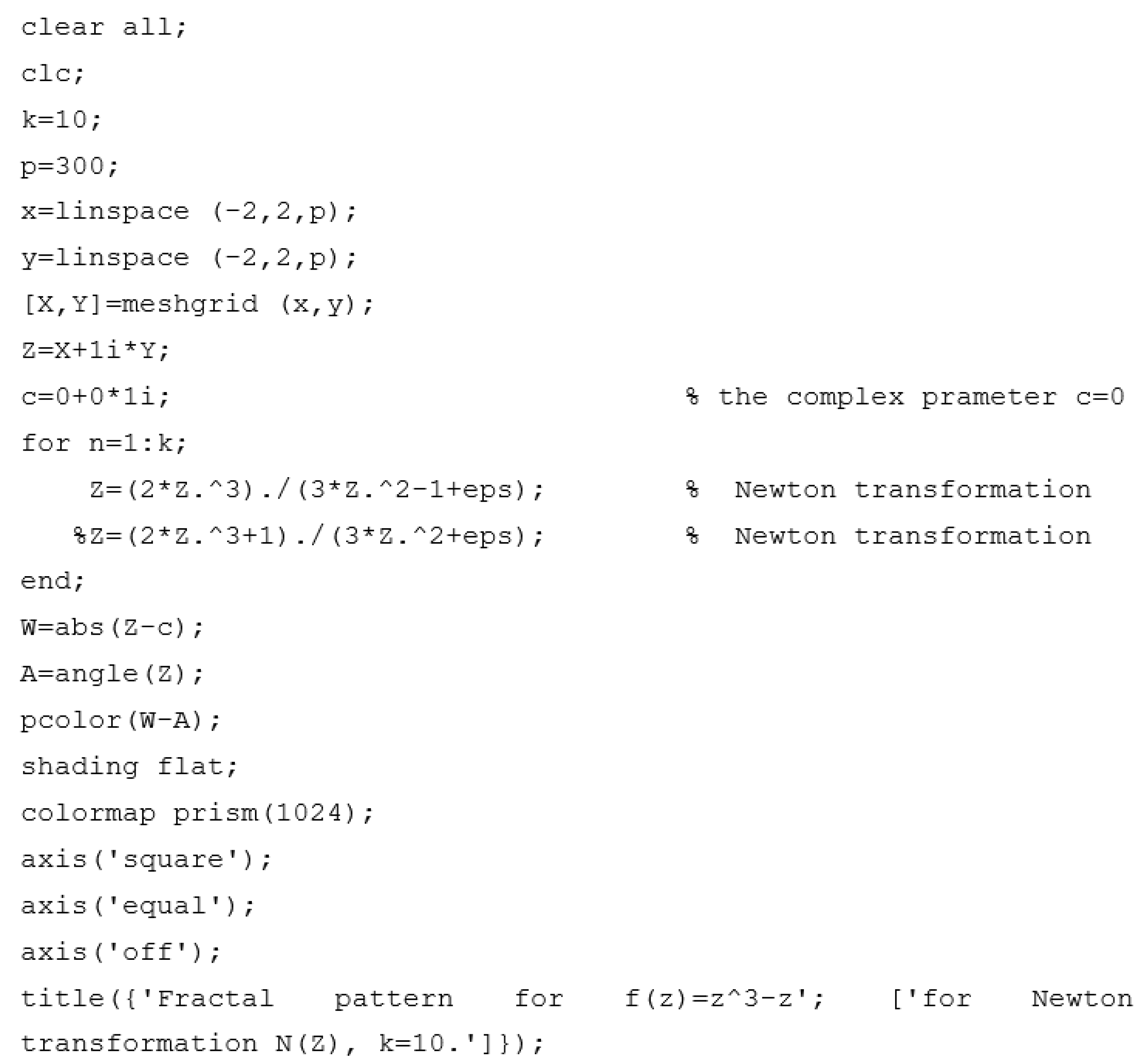
The Pseudo-code of the algorithm is as follows: $cycount=k;$             % k is the cycle count Represent the complex variable z as a couple of real variables in the complex plane, and evaluate each point $z$ on a square mesh grid $\left(-r\le x\le r,–r\le y\le r\right),$$r\in R$ (mesh grid or region).     $z=x+y\ast i;$     $c=a+b\ast i;$ for n = 1 to cycount do            % for loop   $z_n=N\left(z_{n-1}\right);$                 % numerical iteration formulaend end;                                         % end for loop $modulus=\left|z_n\right|;$                 % computes the absolute value of zn Determine colour-value to the various “basins of attraction”. Plot pixel of modulus with colour-value.

Instead of evaluating the number of cycles required so that the $\left|z_n\right|>$ bailout value, the value of $\left|z_n\right|$ for a fixed number of cycles is evaluated. To make it clear, we present now what is the pseudo-code of the so-called modified escape time algorithm that employs that theory.

This algorithm is a variation on the escape time algorithm, which makes the interior structure of the resulting pattern of the applied numerical iteration formula to $f(z)$ more informative, and reduces the computation because it avoids the conditional instructions speeding up the computer program’s execution.

3. Results

We have utilized Newton’s method to find the roots of a complex-valued function. Through the aid of MATLAB, the complex basins of attraction for several complex-valued functions can be viewed and the following fractal patterns (Figure 1, Figure 2, Figure 3 and Figure 4) can be obtained. These fractal patterns are called Newton fractals [2,3,6,11]. They are a fractal based on using Newton’s method in order to find roots for a particular complex-valued function starting from points laid out on a region (the two-dimensional grid of points) in the complex plane $ℂ$. We ran Newton’s method, starting from each grid point, and we determined to which one of the roots it was converging for this grid point.

4. Discussion

Figure 1 is one solution to the problem of dividing a plane into three regions so that all three regions share a common boundary. The infinitely loop set that is the common boundary is called a fractal pattern. The Newton transformation $N(z)=2z^3/(3z^2-1)$ takes the fractal pattern onto itself, and does so chaotically. It also preserves each of the three colored regions and transforms them in interesting ways [16]. For example, $N$ takes the yellow bulb at around $z=0.5$ into the main yellow region on the left. Figure 2 is the detail of a bulb from Figure 1.

A fixed point is a point that is mapped to itself under an iterated function [12]. The three roots to the cubic complex-valued function $z^3-1$ are mapped to themselves under the iterative Newton’s method. A fixed point is an attractive fixed point if all points in a neighborhood around it converge towards it [11]. All points that converge to a fixed point form a basin of attraction for the point.

Figure 3 is an example that shows a part of the basins for Newton’s method applied to the cubic complex-valued function $z^3-1.$ $B(1)$ is in yellow, and the other two basins are in the other two colors.

Figure 4 shows the basin of attraction of the roots when Newton’s method is applied to $z^5-z^2=z^2(z^3-1).$ Since 0 is a double root of $f(z)$, and $|N^{\prime }(0)|=1$, this means that the double root 0 is an indifferent (may be attracting, repelling, or neither) fixed point for $N(z)$, and any neighborhood of such fixed point contains points that are in the basin of attraction of that indifferent fixed point and points that are not in that basin, because Newton’s method converges only linearly at the double root.

Finally, in Figure 1, Figure 3 and Figure 4 we use a square grid $\left(-r\le x\le r,–r\le y\le r\right),$ where $r\in R$ is mesh grid or region. To speed up the convergence rate, we avoided conditional instructions of the prior escape time algorithm and used a maximum of 10 iterations to reach a fractal pattern when iterating Newton’s method via modified escape time algorithm. This conclusively shows that the results are superior in terms of performance and algorithmic efficiency.

5. Conclusions

The mathematical foundations behind generating a fractal pattern of an algebraic function using the numerical iteration method have been introduced. For constructing a fractal pattern, we first introduced the numerical iterative method for the complex plane and described a modified algorithm that shows the dynamical behavior of the numerical iteration method (see the result in Section 3).

This algorithm is based on the fact that it identifies the fractal pattern generated by the numerical iteration method as the boundary of the points that are attracted to infinity and the points that are attracted to an attracted k–cycle of the algebraic function.

This algorithm speeds up the convergence rate by avoiding conditional instructions and minimizing the number of iterations needed to obtain the fractal pattern to 10 iterations.

This algorithm is a variation of the escape time algorithm, which changes the interior structure of the fractal pattern of the numerical iteration method applied to the algebraic function for accelerating the fractal pattern generation.

The most used iteration method is Newtons’ iteration formula, but other famous iteration methods could be introduced for future works—e.g., Chun-Hui He’s iteration method, the variational iteration method, and the homotopy perturbation method. The values of the fractal dimensions of the fractal pattern could be approximated in future studies. The two-scale fractal dimensions (see [17,18,19]) could be used for this purpose.

This article presented a novel tool making use of the modified escape time algorithm. To accelerate convergence, we removed conditional instructions in the prior algorithm and employed a maximum of 10 iterations to reach a fractal pattern by iterating Newton’s method using the modified escape time algorithm. Our results are superior to both old and recent results in terms of the performance and efficiency of the modified escape time algorithm, and superior results came about in the nonstandard convergence test when Newton’s method was iterated by the modified escape time algorithm, which is a mathematical insight gained in this article. The results give notably new insights into the treatment of fractal pattern generation, which is one of the study’s strengths.

References

1. Mandelbrot, B.B. The Fractal Geometry of Nature; W.H. Freeman & Company: New York, NY, USA, 1999. [Google Scholar]
2. Falconer, K. Fractal Geometry-Mathematical Foundations and Applications; John Wiley & Sons Ltd.: Hoboken, NJ, USA, 1999. [Google Scholar]
3. Gilbert, W.J. Newton’s method for multiple roots. J. Comput. Graph. 1994, 18, 227–229. [Google Scholar] [CrossRef]
4. Mathews, J.H.; Fink, K.D. Numerical Methods Using Matlab; Prentice-Hall: Hoboken, NJ, USA, 1999. [Google Scholar]
5. Al-shameri, W.F.H. Approximating Lyapunov exponents of a discrete dynamical system. Nanosci. Nanotechnol. Lett. 2019, 11, 1612–1615. [Google Scholar] [CrossRef]
6. Al-shameri, W.F.H. A revised algorithm that generates Julia sets using Newton’s method. SUJST 2004, 1, 55–63. [Google Scholar]
7. Al-shameri, W.F.H. Deterministic algorithm for constructing fractal attractors of iterated function systems. Eur. J. Sci. Res. 2015, 134, 121–131. [Google Scholar]
8. Al-shameri, W.F.H. On Nonlinear Iterated Function Systems. Ph.D. Thesis, University of Al-Mustansiriyah, Baghdad, Iraq, 2001. [Google Scholar]
9. Barnsley, M.F. Fractals Everywhere, 2nd ed.; revised with the assistance of and a foreword by Hawley Rising, III; Academic Press: Boston, MA, USA, 1993. [Google Scholar]
10. Al-shameri, W.F.H. Existence of the attractor of a recurrent iterated function system. J. Eng. Appl. Sci. 2019, 14, 182–187. [Google Scholar]
11. Devaney, R.L. Introduction to Chaotic Dynamical Systems; Addison-Wesley: Menlo Park, CA, USA, 1989. [Google Scholar]
12. Gulick, D. Encounters with Chaos; McGraw-Hill: New York, NY, USA, 1992. [Google Scholar]
13. Norton, A. The Julia sets in the quarternions. Comp. Graph. 1989, 13, 267–287. [Google Scholar] [CrossRef]
14. Scheinerman, R.E. Invitation to a Dynamical System; Department of Mathematical Sciences, the Johos Hopkins University: Baltimore, MD, USA, 2000. [Google Scholar]
15. Sprott, J.C.; Pickover, C.A. Automatic generation of general quadratic map basins. J. Comput. Graph. 1995, 19, 309–313. [Google Scholar] [CrossRef]
16. Hahn, B.D.; Valentine, D.T. Essential Matlab for Engineers and Scientists; Elsevier Ltd.: Amsterdam, The Netherlands, 2019. [Google Scholar]
17. He, C.-H.; Liu, C. A modified frequency-amplitude formulation for fractal vibration systems. Fractals 2021, 25, 463. [Google Scholar] [CrossRef]
18. Zuo, Y.-T.; Liu, H.-J. Fractal approach to mechanical and electrical properties of graphene/sic composites. Facta Univ.-Ser. Mech. Eng. 2021, 19, 271–284. [Google Scholar] [CrossRef]
19. Liu, F.; Zhang, T.; He, C.-H.; Tian, D. Thermal oscillation arising in a heat shock of a porous hierarchy and its application. Facta Univ. Ser. Mech. Eng. 2021, 19, 4. Available online: http://casopisi.junis.ni.ac.rs/index.php/FUMechEng/article/view/7573 (accessed on 20 January 2022). [CrossRef]
Figure 1. Newton basins for z 3 z .
Fractalfract 06 00196 g001
Figure 2. Detailed of a bulb from Figure 1.
Fractalfract 06 00196 g002
Figure 3. Newton basins for z 3 1 .
Fractalfract 06 00196 g003
Figure 4. Newton basins for z 5 z 2 .
Fractalfract 06 00196 g004
Publisher’s Note: MDPI stays neutral with regard to jurisdictional claims in published maps and institutional affiliations.