A Chebyshev Collocation Approach to Solve Fractional Fisher–Kolmogorov–Petrovskii–Piskunov Equation with Nonlocal Condition

Abstract

We provide a detailed description of a numerical approach that makes use of the shifted Chebyshev polynomials of the sixth kind to approximate the solution of some fractional order differential equations. Specifically, we choose the fractional Fisher–Kolmogorov–Petrovskii–Piskunov equation (FFKPPE) to describe this method. We write our approximate solution in the product form, which consists of unknown coefficients and shifted Chebyshev polynomials. To compute the numerical values of coefficients, we use the initial and boundary conditions and the collocation technique to create a system of equations whose number matches the unknowns. We test the applicability and accuracy of this numerical approach using two examples.

1. Introduction

A study of generalized derivatives and integrals has gained considerable popularity in the last few years, mainly due to its attractive applications in numerous diverse fields such as fluid flow [1], finance [2] and physics [3]. These generalized derivatives and integrals are called fractional derivatives and integrals, respectively [4,5,6]. They are more flexible for real-world applications since they can have both integer and noninteger operators. Fractional derivatives are well-known for their utility in describing the memory and heredity features of a variety of materials and processes [7,8,9,10]. Nikan et al. [11] considered the fractional nonlinear sine-Gordon and Klein–Gordon models arising in relativistic quantum mechanics. Babaei et al. [12] introduced a class of time-fractional stochastic heat equations driven by Brownian motion. Numerical solution of time fractional convection–diffusion-wave equation based on RBF method is described in [13,14]. Zaky et al. [15] applied some pseudospectral methods for solving the Riesz space-fractional Schrödinger equation. Lately, countless researchers are contributing to new models based on fractional equations. Among which, the generalized Fisher–Kolmogorov–Petrovskii–Piskunov equation has substantial attention [16,17,18,19].

In this paper, we introduce the FFKPPE in the form

$${}_0{\mathcal{D}}_t^{\eta }u(x,t)=\mu \Delta u(x,t)+\beta \nabla u(x,t)+\frac{\kappa }{\zeta }{\int }_0^t{e}^{-\frac{t-s}{\zeta }}\Delta u(x,\mathrm{s})\mathrm{ds}+\mathcal{F}(x,t,u),$$

(1)

where $(x,t)\in {\Omega }_{\mathtt{L}}\times {\Omega }_{\mathtt{T}}$, with the following initial and boundary conditions

$$\begin{array}{cc}\hfill & u(x,0)=u_0\left(x\right),x\in {\Omega }_{\mathtt{L}},\hfill \end{array}$$

(2)

$$\begin{array}{cc}\hfill & \mathtt{g}\left(u(0,t)\right)={\rho }_0\left(t\right),t\in {\Omega }_{\mathtt{T}},\hfill \end{array}$$

(3)

$$\begin{array}{cc}\hfill & \widehat{\theta }u(\mathtt{L},t)+\widehat{\delta }{u}_x(\mathtt{L},t)={\rho }_{\mathtt{L}}\left(t\right),t\in {\Omega }_{\mathtt{T}},\hfill \end{array}$$

(4)

where $\Delta :=\frac{{\partial }^2}{\partial x^2}$ is the Laplace operator and $\nabla :=\frac{\partial }{\partial x}$. Further, $\mu$, $\beta$, $\kappa$, $\zeta \ne 0$, $\widehat{\theta }$ and $\widehat{\delta }$ are given real constants. Moreover, ${\Omega }_{\mathtt{L}}:=[0,\mathtt{L}]$, ${\Omega }_{\mathtt{T}}:=[0,\mathtt{T}]$, the nonlinear source term $\mathcal{F}(x,t,u)\in {\mathbf{C}}^1({\Omega }_{\mathtt{L}}\times {\Omega }_{\mathtt{T}}\times \mathbb{R})$ fulfills the Lipschitz condition in terms of u and $u_0\left(x\right)$, ${\rho }_0\left(t\right)$ and ${\rho }_{\mathtt{L}}\left(t\right)$ are regarded as known continuous functions. In addition, the nonlinear function $\mathtt{g}$ of $u(0,t)$ is given and the operator ${}_0{\mathcal{D}}_t^{\eta }[·]$ denotes the Caputo fractional derivative of order $\eta \in (0,1)$ defined as [20]:

$$\begin{array}{c}\hfill {}_0{\mathcal{D}}_t^{\eta }u(x,t)=\frac{1}{\Gamma (1-\eta )}{\int }_0^t{(t-s)}^{-\eta }{u}_s(x,s)\mathrm{d}s,\end{array}$$

(5)

in which $\Gamma (·)$ denotes the Gamma function. The generalized FFKPPE (1), belongs to the class of reaction–diffusion equations. It is commonly used to represent practical situations that often arise in physics, chemistry and biology [18,19,21]. A more specific example is in the modeling of genetic behavior in the growth of micro-organisms [22].

In the literature, the problem (1)–(4) has been considered analytically and numerically. For instance, Araújo et al. [23] investigated the stability of the model represented by (1), while also investigating the qualitative features of its solutions obtained under Dirichlet boundary conditions. Splitting methods were created for purposes of numerically studying the qualitative nature of the solutions. A list of numerical approaches has been proposed and studied for different cases of the Equation (1). Branco et al. [16] studied the approach of method of lines for the numerical solution to integro-differential equation of type (1). In their work, Araújo et al. [24] developed the famous Fisher equation by investigating the qualitative features of the numerical traveling wave solutions of integro-differential equations. The hyperbolic equation equivalence was used to replace the integro-differential equation, allowing for the numerical quantification of the velocity of traveling wave solutions. While studying the effects on memory factors in phenomena of diffusion [25] developed approximation methods for computing integro-differential equations. Barbeiro and Ferreira [26] provided mathematical models to describe medication absorption through the skin. The development of these models involved extending the traditional Fick’s law by incorporating a memory term. This replaces the classical models of advection–diffusion equations with integro-differential equations. The well-posedness of model was investigated using Neumann, Dirichlet and natural boundary conditions. The methods for computing numerical solutions were proposed. In addition, their stability and convergence were studied, while including a presentation of numerical simulations to illustrate the behavior of the model. Khuri and Sayfy proposed a numerical scheme to solve a generalized Fisher integro-differential equation using finite differences and spline collocation in [17]. To manage the numerical integration, a composite weighted trapezoidal rule was used, resulting in a closed-form difference scheme. To assess the method’s accuracy, multiple test examples were solved. The scheme’s convergence and stability were also explored. Babaei et al. sets up a numerical technique that makes use of the Chebyshev polynomials of the sixth kind with the main purpose of approximating the solutions of integro-differential equations of variable order [27]. The sixth-kind Chebyshev polynomials are a special case of the general nonsymmetric class mentioned in [28,29].

We subdivide our research under different headings as follows. In the next section, we focus on fundamental mathematical concepts that lay important groundwork for the subsequent sections. Section 3 outlines the methodology that we use to conduct our research and in the fourth section we study the convergence of this methodology. In Section 5, we apply the methodology to specific examples. We mention our findings and give suggestions in the last section of this manuscript.

2. Preliminaries

For use in sequel, this section presents the basic properties of the sixth-kind Chebyshev polynomials and related necessary definitions.

Definition 1.

We define the Riemann–Liouville fractional integral with order $\eta \in (0,1)$ as [20]

$${\mathrm{I}}_t^{\eta }u(x,t)=\frac{1}{\Gamma \left(\eta \right)}{\int }_0^{t}u(x,s){(t-s)}^{\eta -1}\mathrm{d}s.$$

Definition 2

([12]). The following recurrence relation is used to obtain the sixth-kind Chebyshev polynomials ${\widehat{\varphi }}_q\left(t\right)$

$${\widehat{\varphi }}_0\left(t\right)=1,{\widehat{\varphi }}_1\left(t\right)=t,$$

$${\widehat{\varphi }}_{q+1}\left(t\right)=t{\widehat{\varphi }}_q\left(t\right)+{\varrho }_q{\widehat{\varphi }}_{q-1}\left(t\right),q=2,3,\dots ,$$

where

$${\varrho }_q:=\frac{-(q+1-{(-1)}^q)(q+2-{(-1)}^q)}{4(q+1)(q+2)}.$$

Definition 3

([29]). Considering the interval $[0,\mathtt{T}]$, then the shifted sixth-kind Chebyshev polynomials are written as

$${\varphi }_q\left(t\right)={\widehat{\varphi }}_q((2/\mathtt{T})t-1),q=0,1,2,\dots$$

In analytical format, these polynomials are presented as [29]

$${\varphi }_q\left(t\right)=\sum _{k=0}^q{\mathcal{L}}_{k,q}{t}^k,$$

(6)

where

$${\mathcal{L}}_{k,q}=\left\{\begin{array}{cc}\begin{array}{c}\begin{array}{cc}\frac{2^{2k-q}}{(2k+1)!{\mathtt{T}}^k}\sum _{p=\lfloor \frac{k+1}{2}\rfloor }^{\frac{q}{2}}{\displaystyle \frac{{(-1)}^{\frac{q}{2}+p+k}(2p+k+1)!}{(2p-k)!}},& \end{array}\end{array}\hfill & qeven,\\ \frac{2^{2k-q+1}}{(2k+1)!(q+1){\mathtt{T}}^k}\sum _{p=\lfloor \frac{k}{2}\rfloor }^{\frac{q-1}{2}}{\displaystyle \frac{{(-1)}^{\frac{q+1}{2}+p+k}(p+1)(2p+k+2)!}{(2p-k+1)!}},& qodd.\end{array}\right.$$

Let ${\mathbf{L}}_{\varpi }^2\left({\Omega }_{\mathtt{L}}\times {\Omega }_{\mathtt{T}}\right)$ represent a space that consists of square integrable functions having variables $(x,t)$ and the weight function $\varpi (x,t)=w\left(x\right)w\left(t\right)$ with $w\left(x\right)=\sqrt{x-x^2}{(2x-1)}^2$.

Theorem 1.

We assume that $f(x,t)\in {\mathbf{L}}_{\varpi }^2\left({\Omega }_{\mathtt{L}}\times {\Omega }_{\mathtt{T}}\right)$ satisfies the expansion [12]

$$f(x,t)=\sum _{p=0}^{\infty }\sum _{q=0}^{\infty }{c}_{p,q}{\varphi }_p\left(x\right){\varphi }_q\left(t\right).$$

Suppose ${∥\frac{{\partial }^{6}f(x,t)}{\partial x^3\partial t^3}∥}_2\le \widehat{c}$ and $\widehat{c}>0$. The inequality $|c_{p,q}|<\frac{\widehat{c}}{p^3{q}^3}$ for all $p,q>3$, is satisfied for the expansion coefficients. Further, if

$$f(x,t)\simeq f_{n,m}(x,t)=\sum _{p=0}^n\sum _{q=0}^m{c}_{p,q}{\varphi }_p\left(x\right){\varphi }_q\left(t\right),$$

(7)

is an estimate for $f(x,t)$, then

$$|f(x,t)-f_{n,m}(x,t)|<\frac{\widehat{c}}{2^{n+m}},$$

$$|\nabla f(x,t)-\nabla f_{n,m}(x,t)|<\sigma \frac{n}{2^{n+m-2}},$$

$$|\Delta f(x,t)-\Delta f_{n,m}(x,t)|<\widehat{\sigma }\frac{n^3}{2^{n+m-8}},$$

where σ, $\widehat{\sigma }$$>0$.

Definition 4.

Suppose ${\mathrm{P}}_{p+1}\left(t\right)$ is Legendre polynomial of order $p+1$ on $[-1,1]$. The Legendre–Gauss quadrature formula for $g\left(t\right)\in \mathbf{C}[a,b]$ is defines as:

$${\int }_a^{b}g\left(t\right)\mathrm{d}t=\frac{b-a}{2}\sum _{r=0}^{\mathrm{M}}{\mathtt{w}}_{r}g(\frac{b-a}{2}{\varsigma }_r+\frac{b+a}{2}),$$

in which distinct nodes ${\left\{{\varsigma }_r\right\}}_{r=0}^{\mathrm{M}}$ are the zeros of ${\mathrm{P}}_{\mathrm{M}+1}\left(t\right)$ and ${\left\{{\mathtt{w}}_r\right\}}_{r=0}^{\mathrm{M}}$ are the corresponding weights [30]

$${\mathtt{w}}_r=\frac{2}{(1-{\varsigma }_r^2){\left({\mathrm{P}}_{\mathrm{M}+1}^{\prime }\left({\varsigma }_r\right)\right)}^2}.$$

3. Numerical Method

In this section, we describe numerical technique for solving (1)–(4) on the basis of the shifted sixth-kind Chebyshev polynomials. We obtain the numerical approximation of Equation (1) by considering an approximation of the fractional derivative of the unknown function as:

$${}_0{\mathcal{D}}_t^{\eta }u(x,t)\simeq {}_0{\mathcal{D}}_t^{\eta }{u}_{n,m}(x,t)=\sum _{p=0}^n\sum _{q=0}^m{c}_{p,q}{\varphi }_p\left(x\right){\varphi }_q\left(t\right)=\Phi {\left(x\right)}^{\mathrm{T}}\mathbf{C}\Phi \left(t\right),$$

(8)

in which

$$\begin{array}{cc}\hfill \Phi \left(x\right)& ={[{\varphi }_0\left(x\right),{\varphi }_1\left(x\right),\dots ,{\varphi }_n\left(x\right)]}^{\mathrm{T}},\hfill \end{array}$$

(9)

$$\begin{array}{cc}\hfill \Phi \left(t\right)& ={[{\varphi }_0\left(t\right),{\varphi }_1\left(t\right),\dots ,{\varphi }_m\left(t\right)]}^{\mathrm{T}},\hfill \end{array}$$

(10)

and

$$\mathbf{C}={\left[c_{p,q}\right]}_{(n+1)\times (m+1)},p=0,\dots ,n,q=0,\dots ,m,$$

represent a matrix with unknown entries whose numerical values are to be computed. According to Definition 1 and the initial condition (2)

$$\begin{array}{cc}\hfill u(x,t)& \simeq {\mathrm{I}}_t^{\eta }\left(\Phi {\left(x\right)}^{\mathrm{T}}\mathbf{C}\Phi \left(t\right)\right)+u_0\left(x\right)=\Phi {\left(x\right)}^{\mathrm{T}}\mathbf{C}{\mathrm{I}}_t^{\eta }\Phi \left(t\right)+u_0\left(x\right).\hfill \end{array}$$

By applying Definition 1 and shifted SKCPs (6), for $q=0,\dots ,m$

$$\begin{array}{c}\hfill {\Lambda }_q^{\eta }\left(t\right):={\mathrm{I}}_t^{\eta }{\varphi }_q\left(t\right)=\sum _{k=0}^q{\mathcal{L}}_{k,q}{\mathrm{I}}_t^{\eta }\left(t^k\right)=\sum _{k=0}^q{\mathcal{L}}_{k,q}^{\eta }{t}^{k+\eta },\end{array}$$

where ${\mathcal{L}}_{k,q}^{\eta }:={\mathcal{L}}_{k,q}\frac{\Gamma (k+1)}{\Gamma (k+1+\eta )}$, thus, we let

$$\begin{array}{c}\hfill u(x,t)\simeq u_{n,m}(x,t)=\Phi {\left(x\right)}^{\mathrm{T}}\mathbf{C}{\Phi }_t^{\eta }\left(t\right)+u_0\left(x\right),\end{array}$$

(11)

such that

$${\Phi }_t^{\eta }\left(t\right):={\left[{\Lambda }_0^{\eta }\left(t\right),{\Lambda }_1^{\eta }\left(t\right),\dots ,{\Lambda }_m^{\eta }\left(t\right)\right]}^{\mathrm{T}}.$$

(12)

According to (1) and (11)

$$\begin{array}{cc}\hfill \mathbf{R}(x,t)& :=\Phi {\left(x\right)}^{\mathrm{T}}\mathbf{C}\Phi \left(t\right)-\mu \left({\Phi }_{xx}{\left(x\right)}^{\mathrm{T}}\mathbf{C}{\Phi }_t^{\eta }\left(t\right)+u_0^{″}\left(x\right)\right)\hfill \\ \hfill & -\beta \left({\Phi }_x{\left(x\right)}^{\mathrm{T}}\mathbf{C}{\Phi }_t^{\eta }\left(t\right)+u_0^{\prime }\left(x\right)\right)\hfill \\ \hfill & -\frac{\kappa }{\zeta }{\int }_0^t{e}^{-\frac{t-s}{\zeta }}\left({\Phi }_{xx}{\left(x\right)}^{\mathrm{T}}\mathbf{C}{\Phi }_s^{\eta }\left(s\right)+u_0^{″}\left(x\right)\right)\mathrm{ds}\hfill \\ \hfill & -\mathcal{F}\left(x,t,\Phi {\left(x\right)}^{\mathrm{T}}\mathbf{C}{\Phi }_t^{\eta }\left(t\right)+u_0\left(x\right)\right),\hfill \end{array}$$

(13)

with

$$\begin{array}{cc}\hfill {\Phi }_x\left(x\right)& ={\left[{\varphi }_0^{\prime }\left(x\right),{\varphi }_1^{\prime }\left(x\right),\dots ,{\varphi }_n^{\prime }\left(x\right)\right]}^{\mathrm{T}},\hfill \end{array}$$

(14)

$$\begin{array}{cc}\hfill {\Phi }_{xx}\left(x\right)& ={\left[{\varphi }_0^{″}\left(x\right),{\varphi }_1^{″}\left(x\right),\dots ,{\varphi }_n^{″}\left(x\right)\right]}^{\mathrm{T}}.\hfill \end{array}$$

(15)

In addition, from Equation (11) and the initial and boundary conditions (2)–(4), we define

$$\begin{array}{cc}\hfill \Psi \left(x\right)& :=\Phi {\left(x\right)}^{\mathrm{T}}\mathbf{C}{\Phi }_t^{\eta }\left(0\right)+u_0\left(x\right),\hfill \end{array}$$

(16)

$$\begin{array}{cc}\hfill {\Pi }_1\left(t\right)& :=\mathtt{g}\left(\Phi {\left(0\right)}^{\mathrm{T}}\mathbf{C}{\Phi }_t^{\eta }\left(t\right)+u_0\left(0\right)\right)-{\rho }_0\left(t\right),\hfill \end{array}$$

(17)

$$\begin{array}{cc}\hfill {\Pi }_2\left(t\right)& :=\widehat{\theta }\left(\Phi {\left(\mathtt{L}\right)}^{\mathrm{T}}\mathbf{C}{\Phi }_t^{\eta }\left(t\right)+u_0\left(\mathtt{L}\right)\right)\hfill \\ \hfill & +\widehat{\delta }\left({\Phi }_x{\left(\mathtt{L}\right)}^{\mathrm{T}}\mathbf{C}{\Phi }_t^{\eta }\left(t\right)+u_0^{\prime }\left(\mathtt{L}\right)\right)-{\rho }_{\mathtt{L}}\left(t\right).\hfill \end{array}$$

(18)

Let $x_0=0,x_n=\mathtt{L}$. We denote the roots of ${\varphi }_{n-1}\left(x\right)$ and ${\varphi }_m\left(t\right)$ to be $\{x_p:p=1,\dots ,n-1\}$ and $\{t_q:q=1,\dots ,m\}$, respectively. If we evaluate (16)–(18) at the respective collocation points $(x_p,t_q)$, $p=1,\dots ,n-1$, and $q=1,\dots ,m$, then

$$\begin{array}{cc}\hfill \mathbf{R}(x_p,t_q)& =\Phi {\left(x_p\right)}^{\mathrm{T}}\mathbf{C}\Phi \left(t_q\right)-\mu \left({\Phi }_{xx}{\left(x_p\right)}^{\mathrm{T}}\mathbf{C}{\Phi }_t^{\eta }\left(t_q\right)+u_0^{″}\left(x_p\right)\right)\hfill \\ \hfill & -\beta \left({\Phi }_x{\left(x_p\right)}^{\mathrm{T}}\mathbf{C}{\Phi }_t^{\eta }\left(t_q\right)+u_0^{\prime }\left(x_p\right)\right)\hfill \\ \hfill & -\frac{\kappa }{\zeta }\underset{{\mathcal{E}}_{p,q}}{\underbrace{{\int }_0^{t_q}{e}^{-\frac{t_q-s}{\zeta }}\left({\Phi }_{xx}{\left(x_p\right)}^{\mathrm{T}}\mathbf{C}{\Phi }_s^{\eta }\left(s\right)+u_0^{″}\left(x_p\right)\right)\mathrm{ds}}}\hfill \\ \hfill & -\mathcal{F}\left(x_p,t_q,\Phi {\left(x_p\right)}^{\mathrm{T}}\mathbf{C}{\Phi }_t^{\eta }\left(t_q\right)+u_0\left(x_p\right)\right).\hfill \end{array}$$

(19)

Due to Definition 4, ${\mathcal{E}}_{p,q}$ can be approximated as

$$\begin{array}{cc}\hfill {\mathcal{E}}_{p,q}& ={\int }_0^{t_q}{e}^{-\frac{t_q-s}{\zeta }}\left({\Phi }_{xx}{\left(x_p\right)}^{\mathrm{T}}\mathbf{C}{\Phi }_s^{\eta }\left(s\right)+u_0^{″}\left(x_p\right)\right)\mathrm{ds}\hfill \\ \hfill & =\frac{t_q}{2}\sum _{r=0}^{\mathrm{M}}{\mathtt{w}}_r\left(e^{-\frac{t_q-s_{r,q}}{\zeta }}\left({\Phi }_{xx}{\left(x_p\right)}^{\mathrm{T}}\mathbf{C}{\Phi }_t^{\eta }\left(s_{r,q}\right)+u_0^{″}\left(x_p\right)\right)\right),\hfill \end{array}$$

(20)

where $s_{r,q}=\frac{t_q}{2}{\varsigma }_r+\frac{t_q}{2}.$ Thus, replacing (20) in (19) and considering (16)–(18) at the collocation points $(x_p,t_q)$, yield    

$$\begin{array}{cc}\hfill & \mathbf{R}(x_p,t_q)=0,p=1,\dots ,n-1,q=1,\dots ,m,\hfill \end{array}$$

(21)

$$\begin{array}{cc}\hfill & {\Pi }_1\left(t_q\right)=0,q=1,\dots ,m,\hfill \end{array}$$

(22)

$$\begin{array}{cc}\hfill & {\Pi }_2\left(t_q\right)=0,q=1,\dots ,m,\hfill \end{array}$$

(23)

$$\begin{array}{cc}\hfill & \Psi \left(x_p\right)=0,p=0,\dots ,n.\hfill \end{array}$$

(24)

The relations (21)–(24) imply that we deduce an $(n+1)\times (m+1)$ system of nonlinear equations that can be solved through a numerical approach, such as the Newton iteration technique, to achieve the numerical values of $c_{p,q}$, $p=0,1,\dots ,n$, $q=0,\dots ,m$. The given method in this section is listed as Algorithm 1.

Algorithm 1: Algorithm of presented method in Section 3

Input: $\mathtt{L},\mathtt{T},\mu ,\beta ,\kappa ,\zeta ,\widehat{\theta },\widehat{\delta }$ and $n,m,\mathtt{M}\in {\mathbb{Z}}^{+}$, $\eta \in (0,1)$ and functions F, $\mathtt{g},u_0,{\rho }_0$ and ${\rho }_{\mathtt{L}}$.

Step 1: Compute the shifted sixth-kind Chebyshev polynomials ${\varphi }_i\left(x\right)$ on the interval $[0,\mathtt{L}]$ and ${\varphi }_j\left(t\right)$ on the interval $[0,\mathtt{T}]$.

Step 2: Compute the vector of shifted sixth-kind Chebyshev polynomials $\Phi \left(x\right)$ and $\Phi \left(t\right)$ from Equations (9) and (10).

Step 3: Compute the vectors ${\Phi }_t^{\eta }\left(t\right)$ from (12) and ${\Phi }_x\left(x\right)$, ${\Phi }_{xx}\left(x\right)$ from Equations (14) and (15).

Step 4: Compute the collocation points $x_p$ and $t_q$.

Step 5: Compute the collocation points $s_{r,p}$ and ${\mathtt{w}}_r$.

Step 10: Solve the nonlinear system (21)–(24) and obtain the unknown vector $\mathbf{C}$.

Step 12.4: Let $u_{n,m}(x,t)=\Phi {\left(x\right)}^{\mathrm{T}}\mathbf{C}{\Phi }_t^{\eta }\left(t\right)+u_0\left(x\right)$.

Step 13: Post-processing the results.

Output: The approximate solution: $u(x,t)\simeq u_{n,m}(x,t)$.

4. Convergence Analysis

To further explore the behavior of the obtained numerical solution, this section presents a discussion of how the numerical solution $u_{n,m}(x,t)$ converges towards the exact solution $u(x,t)$.

Theorem 2.

Let $u_{n,m}(x,t)$ be the approximate solution of (1), $u(x,t)$ be its exact solution and ${\mathcal{R}}_{n,m}(x,t)$ be the residual error. Then,

$$\underset{(x,t)\in {\Omega }_{\mathtt{L}}\times {\Omega }_{\mathtt{T}}}{sup}\left|{\mathcal{R}}_{n,m}(x,t)\right|\le \widehat{\rho }\frac{n^3+n+m+1}{2^{n+m-8}},$$

where $\widehat{\rho }$ is a positive constant.

Proof. 

Since $u_{n,m}(x,t)$ is the numerical solution of (1), thus

$$\begin{array}{cc}\hfill {}_0{\mathcal{D}}_t^{\eta }{u}_{n,m}(x,t)& =\mu \Delta u_{n,m}(x,t)+\beta \nabla u_{n,m}(x,t)+\mathcal{F}(x,t,u_{n,m}(x,t))\hfill \\ \hfill & +\frac{\kappa }{\zeta }{\int }_0^t{e}^{-\frac{t-s}{\zeta }}\Delta u_{n,m}(x,\mathrm{s})\mathrm{ds}+{\mathcal{R}}_{n,m}(x,t).\hfill \end{array}$$

(25)

With reference to Equations (1) and (25), we have

$$\begin{array}{cc}\hfill |{\mathcal{R}}_{n,m}(x,t)|& \le |{}_0{\mathcal{D}}_t^{\eta }{\mathbf{e}}_{n,m}(x,t)|+|\mu \left|\right|\Delta {\mathbf{e}}_{n,m}(x,t)|+|\beta \left|\right|\nabla {\mathbf{e}}_{n,m}(x,t)|\hfill \\ \hfill & +|\mathcal{F}(x,t,u(x,t))-\mathcal{F}(x,t,{\mathcal{U}}_{n,m}(x,t))|\hfill \\ \hfill & +|\frac{\kappa }{\zeta }\left|\right|{\int }_0^t{e}^{-\frac{t-s}{\zeta }}\Delta {\mathbf{e}}_{n,m}(x,s)\mathrm{ds}|\hfill \end{array}$$

(26)

where ${\mathbf{e}}_{n,m}(x,t):=u(x,t)-u_{n,m}(x,t)$. Using (5) and Theorem 1, results    

$$\begin{array}{cc}\hfill |{}_0{\mathcal{D}}_t^{\eta }{\mathbf{e}}_{n,m}(x,t)|& \le \frac{1}{\Gamma (1-\eta )}{\int }_0^t\left|{(t-s)}^{-\eta }\right|\left|\frac{\partial {\mathbf{e}}_{n,m}}{\partial s}(x,s)\right|\mathrm{d}s\hfill \\ \hfill & \le \frac{b_1}{\Gamma (1-\eta )}{\int }_0^t\underset{(x,t)\in {\Omega }_{\mathtt{L}}\times {\Omega }_{\mathtt{T}}}{sup}\left|\frac{\partial {\mathbf{e}}_{n,m}}{\partial t}(x,t)\right|\mathrm{d}s\hfill \\ \hfill & \le \widehat{\lambda }\frac{m}{2^{n+m-2}},\hfill \end{array}$$

(27)

where $\widehat{\lambda }=\frac{\sigma b_1\mathtt{T}}{\Gamma (1-\eta )}$ and $b_1$ is a positive constant depended on $\eta$ and $\mathtt{T}$. The function $\mathcal{F}$ fulfills the Lipschitz condition in terms of u, hence

$$|\mathcal{F}(x,t,u(x,t))-\mathcal{F}(x,t,u_{n,m}(x,t))|\le {\xi }_{\mathtt{F}}\left|{\mathbf{e}}_{n,m}(x,t)\right|,$$

where ${\xi }_{\mathtt{F}}>0$. From Theorem 1

$$\begin{array}{c}\hfill |\mathcal{F}(x,t,u(x,t))-\mathcal{F}(x,t,u_{n,m}(x,t))|<\frac{\widehat{c}{\xi }_{\mathtt{F}}}{2^{n+m}}.\end{array}$$

(28)

Moreover,

$$\begin{array}{cc}\hfill |{\int }_0^t{e}^{-\frac{t-s}{\zeta }}\Delta {\mathbf{e}}_{n,m}(x,s)\mathrm{ds}|& \le {\int }_0^t\left|e^{-\frac{t-s}{\zeta }}\right||\Delta {\mathbf{e}}_{n,m}(x,s)|\mathrm{ds}\hfill \\ \hfill & \le b_2{\int }_0^t\underset{(x,t)\in {\Omega }_{\mathtt{L}}\times {\Omega }_{\mathtt{T}}}{sup}|\Delta {\mathbf{e}}_{n,m}(x,s)|\mathrm{ds}\hfill \\ \hfill & \le b_2\mathtt{T}\widehat{\sigma }\frac{n^3}{2^{n+m-8}},\hfill \end{array}$$

(29)

where $b_2$ is a positive constant depended on $\mathtt{T}$. Thus, from relations (26)–(29) and Theorem 1, we obtain

$$\begin{array}{cc}\hfill |{\mathcal{R}}_{n,m}(x,t)|& \le \frac{\widehat{\lambda }m+\left|\beta \right|\sigma n}{2^{n+m-2}}+\left(\right|\mu |\widehat{\sigma }+|\frac{\kappa }{\zeta }\left|b_2\mathtt{T}\widehat{\sigma }\right)\frac{n^3}{2^{n+m-8}}+\frac{\widehat{c}{\xi }_{\mathtt{F}}}{2^{n+m}}\hfill \\ \hfill & \le \frac{\widehat{\lambda }m+\left|\beta \right|\sigma n}{2^{n+m-8}}+\left(\right|\mu |\widehat{\sigma }+|\frac{\kappa }{\zeta }\left|b_2\mathtt{T}\widehat{\sigma }\right)\frac{n^3}{2^{n+m-8}}+\frac{\widehat{c}{\xi }_{\mathtt{F}}}{2^{n+m-8}}\hfill \\ \hfill & \le \widehat{\rho }\frac{n^3+n+m+1}{2^{n+m-8}},\hfill \end{array}$$

in which $\widehat{\rho }=max\{\widehat{\lambda },\left|\beta \right|\sigma ,\left|\mu \right|\widehat{\sigma }+|\frac{\kappa }{\zeta }|b_2\mathtt{T}\widehat{\sigma },\widehat{c}{\xi }_{\mathtt{F}}\}$. As a result

$$\underset{(x,t)\in {\Omega }_{\mathtt{L}}\times {\Omega }_{\mathtt{T}}}{sup}\left|{\mathcal{R}}_{n,m}(x,t)\right|\le \widehat{\rho }\frac{n^3+n+m+1}{2^{n+m-8}}.$$

   □

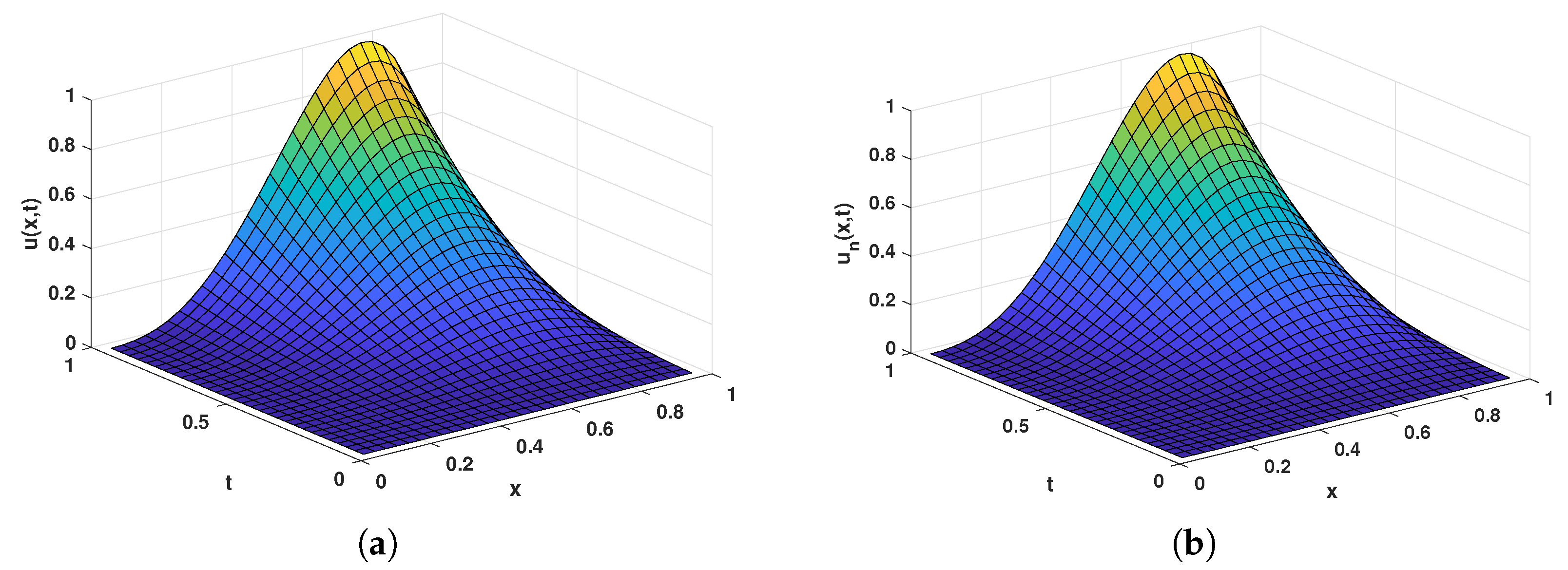
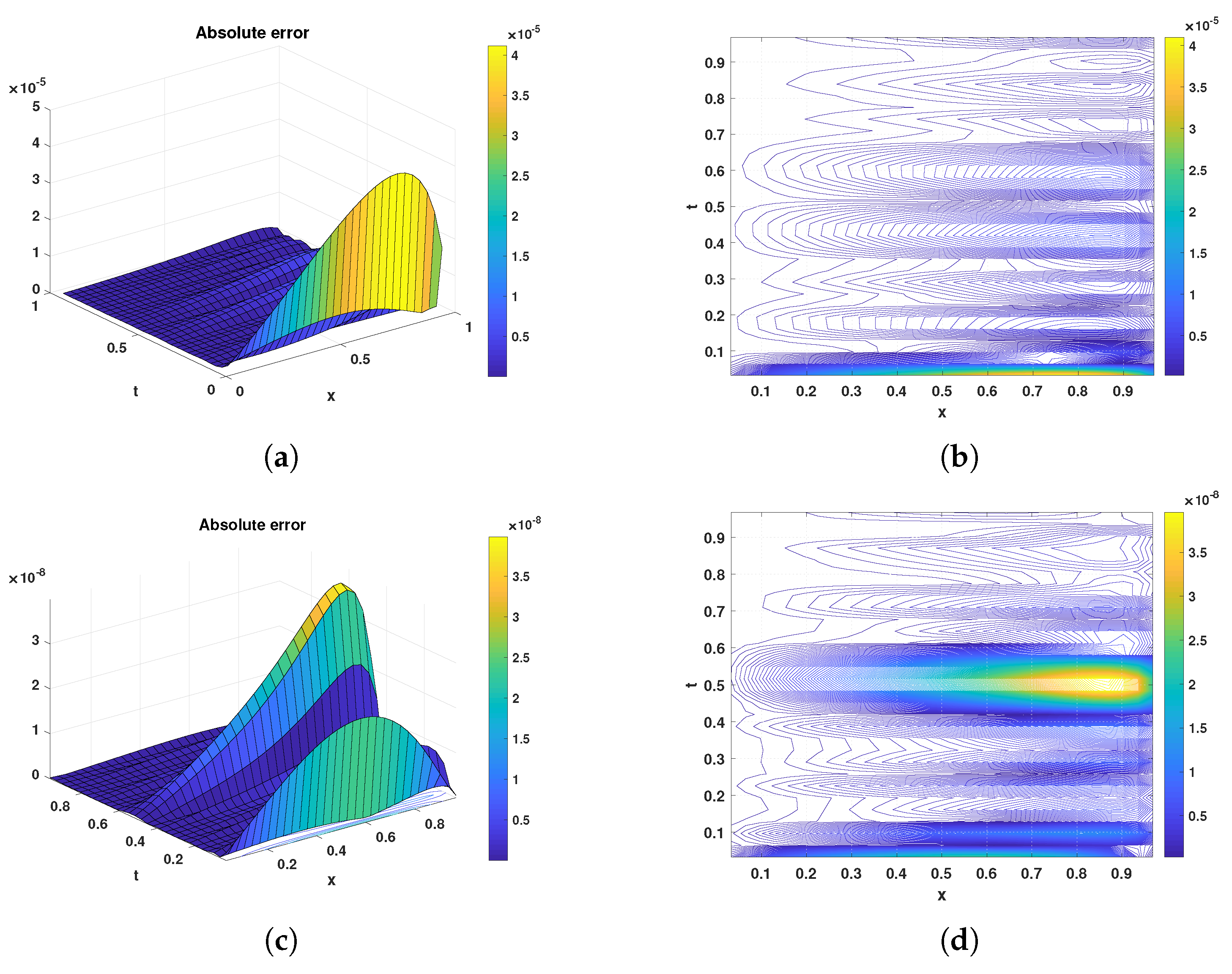
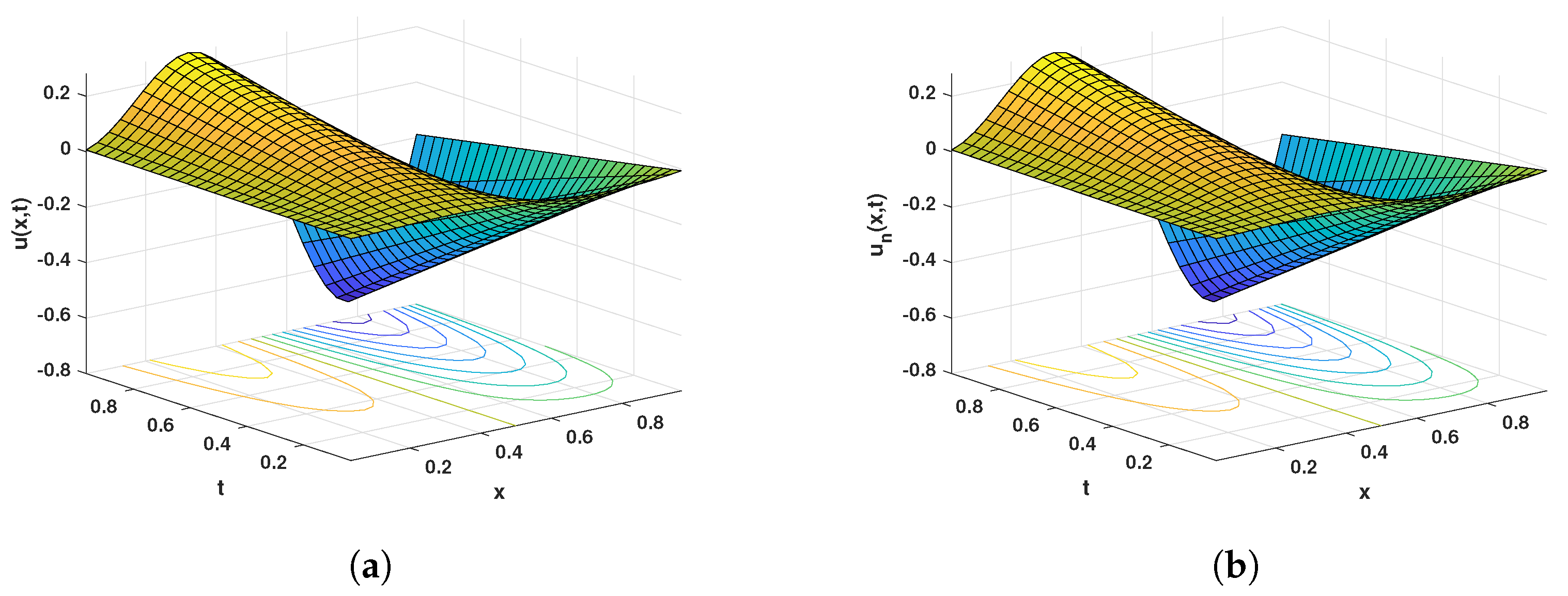
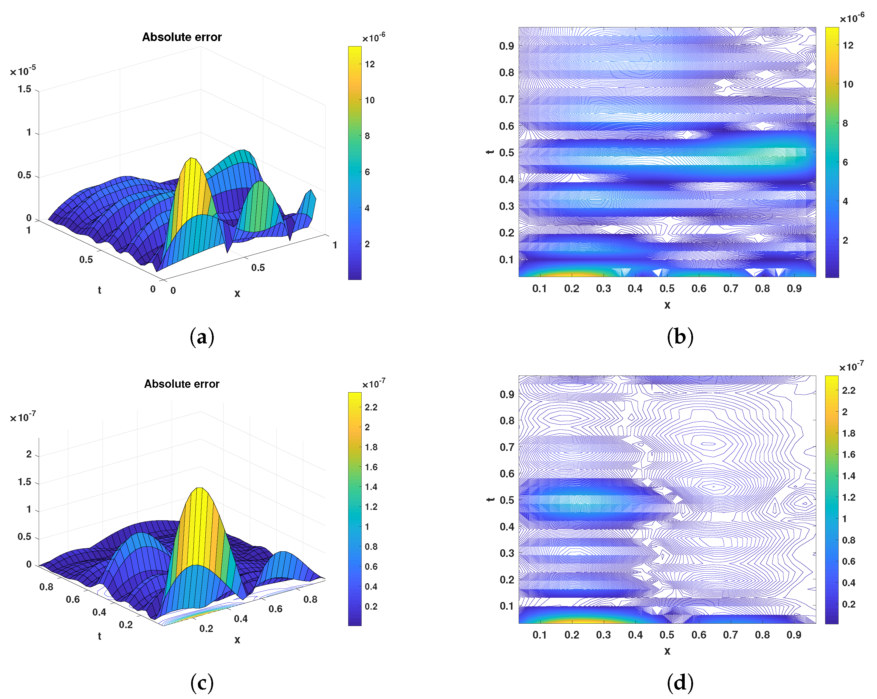
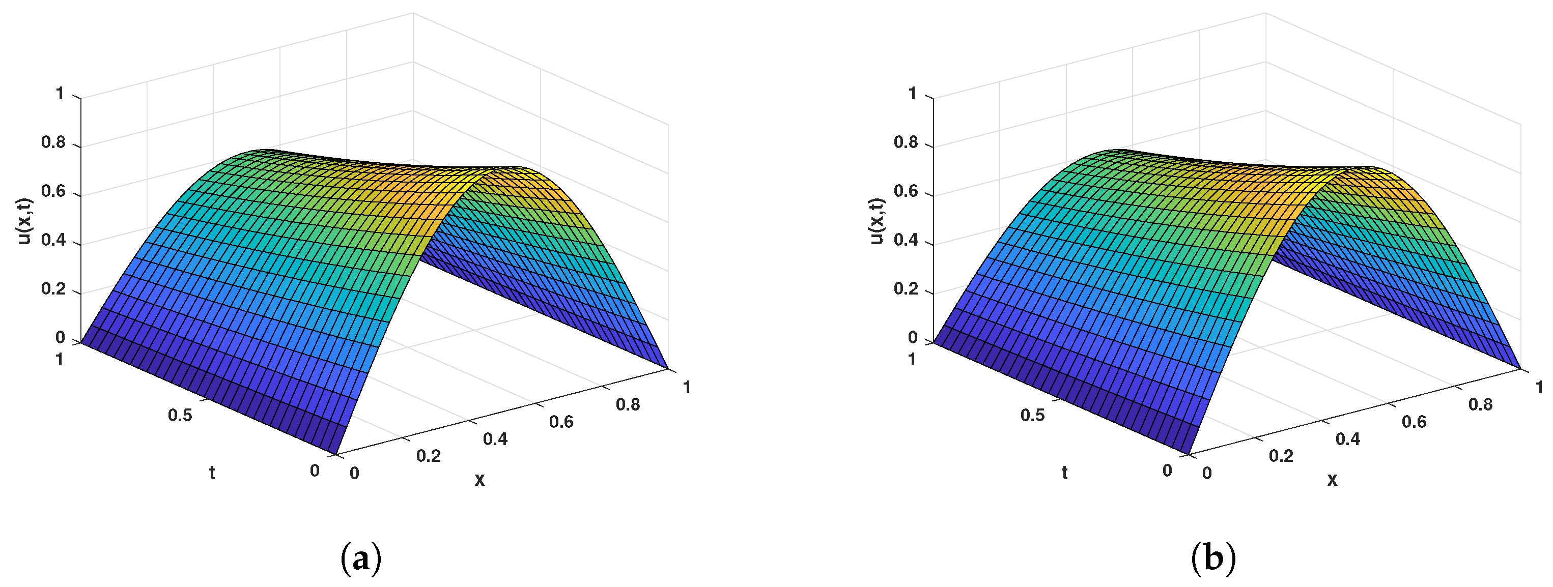
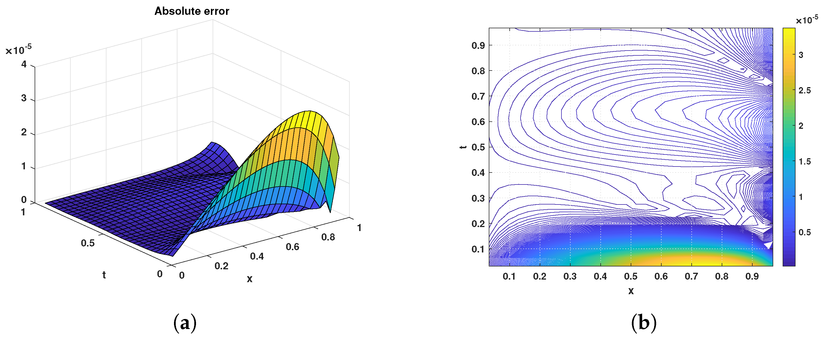
5. Numerical Example

Herein, we implement the described method for solving some numerical examples to investigate the applicability and practical computational efficiency. To assess the accuracy of the scheme, let $n=m$, and the $l_{\infty }$-norm error be given as

$$\parallel {\mathcal{E}}^n{\parallel }_{\infty }=\underset{({\nu }_p,{\tau }_q)}{max}|u({\nu }_p,{\tau }_q)-u_n({\nu }_p,{\tau }_q)|,$$

(30)

where $u_n({\nu }_p,{\tau }_q)$ is an approximate solution of $u(x,t)$ at the designated collocation nodes $x={\nu }_p$, $t={\tau }_q$ and $p,q=1,\dots ,n$. In which case, convergence order (CO) with respect to the $l_{\infty }$-norm is as given by    

$$\mathtt{CO}={log}_{\frac{n_1}{n_2}}\frac{\parallel {\mathcal{E}}^{n_1}{\parallel }_{\infty }}{\parallel {\mathcal{E}}^{n_2}{\parallel }_{\infty }}.$$

(31)

For numerical computations, a personal computer with a 1.70 GHz processor was used. In addition the computational software of choice was MatLab.

Example 1.

Solve the following FFKPPE

$$\begin{array}{c}\hfill {}_0{\mathcal{D}}_t^{\eta }u(x,t)=u_{xx}(x,t)-u_x(x,t)+sin\left(u(x,t)\right)+\frac{1}{5}{\int }_0^t{e}^{-\frac{t-s}{5}}{u}_{xx}(x,\mathrm{s})\mathrm{ds}+f(x,t),\end{array}$$

with ${\Omega }_{\mathtt{L}}={\Omega }_{\mathtt{T}}=[0,1]$ and

$$\begin{array}{cc}\hfill & u(x,0)=0,x\in {\Omega }_{\mathtt{L}},\hfill \\ \hfill & u^2(0,t)=u(\mathtt{L},t)=0,t\in {\Omega }_{\mathtt{T}}.\hfill \end{array}$$

Here, the problem’s exact solution is

$$u(x,t)=10t^2{x}^3(1-x).$$

Figure 1 displays the exact (a) and numerical (b) solutions of $u(x,t)$ for $\eta =0.75$, $\mathtt{M}=5$ and $n=8$. Where as, Figure 2 shows the absolute error and their respective contour plots for $u(x,t)$ given by $n=8$ and $n=10$ when $\eta =0.5$ and $\mathtt{M}=7$. In addition, Table 1 presents convergence results for the numerical solution of $u(x,t)$. These include the convergence order, $l_{\infty }$-norm errors and CPU-time (sec.) for different values of n when $\mathtt{M}=7$.

Figure 1. A diagrammatic comparison of the exact and numerical solutions for Example 1 with $\eta =0.75$. (a) Exact solution; (b) Numerical solution.

Figure 2. Plots indicating absolute errors and error contours for $u(x,t)$, given $n=8$ and $n=10$, with $\eta =0.5$ in the domain $\Omega$ for Example 1. (a) Absolute error with $n=8$; (b) Error contour with $n=8$; (c) Absolute error with $n=10$; (d) Error contour with $n=10$.

Table 1. Convergence analysis results for different values of n for Example 1.

	$\mathit{\eta }=0.25$		$\mathit{\eta }=0.75$
$\mathit{n}$	$\mathbf{\parallel }{\mathcal{E}}^{\mathit{n}}{\mathbf{\parallel }}_{{}_{\mathbf{\infty }}}$	CO	$\mathbf{\parallel }{\mathcal{E}}^{\mathit{n}}{\mathbf{\parallel }}_{{}_{\mathbf{\infty }}}$	CO	CPU-Time
3	$4.0670\times {10}^{-2}$	–	$3.6422\times {10}^{-2}$	–	$2.277$
6	$1.6720\times {10}^{-3}$	$4.6042$	$5.4643\times {10}^{-4}$	$6.0586$	$7.534$
9	$4.0740\times {10}^{-5}$	$9.1613$	$1.0513\times {10}^{-5}$	$9.7436$	$33.884$
12	$5.0991\times {10}^{-7}$	$15.2277$	$1.1055\times {10}^{-07}$	$15.8333$	$76.46$

Example 2.

Solve the following FFKPPE

$$\begin{array}{c}\hfill {}_0{D}_t^{\eta }u(x,t)=-u_{xx}(x,t)+u^2(x,t)+{\int }_0^t{e}^{-(t-s)}{u}_{xx}(x,\mathrm{s})\mathrm{ds}+f(x,t),\end{array}$$

where ${\Omega }_{\mathtt{L}}={\Omega }_{\mathtt{T}}=[0,1]$ and

$$\begin{array}{cc}\hfill & u(x,0)=0,x\in {\Omega }_{\mathtt{L}},\hfill \\ \hfill & u(0,t)=0,x\in {\Omega }_{\mathtt{T}},\hfill \\ \hfill -& u(1,t)+u_x(1,t)=2\pi t,t\in {\Omega }_{\mathtt{T}}.\hfill \end{array}$$

Here, the problem’s exact solution is given by

$$u(x,t)=txsin\left(2\pi x\right).$$

Figure 3 displays plots for the exact (a) and numerical (b) solutions of $u(x,t)$ when $\eta =0.5$, $\mathtt{M}=5$ and $n=8$. Whereas the Figure 4 shows plots for the absolute errors and their respective contour plots for $u(x,t)$ given $n=4$ and $n=8$, when $\eta =0.65$ and $\mathtt{M}=7$. In addition, Table 2 presents convergence results for the numerical solution of $u(x,t)$. These include $l_{\infty }$-norm errors, the convergence order as well as CPU run time in seconds (s) for different values of n when $\mathtt{M}=6$.

Figure 3. A diagrammatic comparison of the exact and numerical solutions for Example 2 with $\eta =0.5$. (a) Exact solution; (b) Numerical solution.

Figure 4. Plots indicating absolute errors and error contours for $u(x,t)$ with $n=12$ and $n=15$ when $\eta =0.65$ in $\Omega$ for Example 2. (a) Absolute error with $n=12$; (b) Error contour with $n=12$; (c) Absolute error with $n=15$; (d) Error contour with $n=15$.

Table 2. Convergence analysis results for different values of n for Example 2.

	$\mathit{\eta }=0.25$		$\mathit{\eta }=0.75$
$\mathit{n}$	$\mathbf{\parallel }{\mathit{E}}^{\mathit{n}}{\mathbf{\parallel }}_{{}_{\mathbf{\infty }}}$	CO	$\mathbf{\parallel }{\mathit{E}}^{\mathit{n}}{\mathbf{\parallel }}_{{}_{\mathbf{\infty }}}$	CO	CPU-Time
3	$6.3855\times {10}^{-1}$	$-$	$3.7469\times {10}^{-1}$	$-$	$2.34$
6	$3.4551\times {10}^{-2}$	$4.2080$	$8.2972\times {10}^{-2}$	$5.4969$	$4.215$
9	$2.5097\times {10}^{-3}$	$6.4673$	$1.8042\times {10}^{-4}$	$9.4419$	$15.116$
12	$7.2113\times {10}^{-5}$	$12.3389$	$5.2019\times {10}^{-6}$	$12.3271$	$70.638$

Example 3.

Solve the following generalized Fisher–Kolmogorov–Petrovskii–Piskunov [17]

$$\begin{array}{c}\hfill u_t(x,t)=-\frac{1}{2{\pi }^2}{u}_{xx}(x,t)+u^2(x,t)+{\int }_0^t{e}^{-\frac{(t-s)}{2}}{u}_{xx}(x,\mathrm{s})\mathrm{ds}+f(x,t),\end{array}$$

where $(x,t)\in (0,1)\times (0,1]$ and

$$\begin{array}{cc}\hfill & u(x,0)=sin\left(\pi x\right),x\in [0,1],\hfill \\ \hfill & u(0,t)+u_x(0,t)=\pi e^{-t/2},t\in (0,1],\hfill \\ \hfill & u(1,t)+u_x(1,t)=-\pi e^{-t/2},t\in (0,1].\hfill \end{array}$$

Here, the problem’s exact solution is given by

$$u(x,t)=e^{-t/2}sin\left(\pi x\right).$$

Figure 5 displays plots for the exact (a) and numerical (b) solutions of $u(x,t)$ when $\mathtt{M}=7$ and $n=12$. Figure 6 shows plots for the absolute error and contour plot for $u(x,t)$, when $n=12$ and $\mathtt{M}=7$.

Figure 5. A diagrammatic comparison of the exact and numerical solutions for Example 3 with $n=12$. (a) Exact solution; (b) Numerical solution.

Figure 6. Plots indicating absolute errors and error contours for $u(x,t)$ with $n=12$ for Example 3. (a) Absolute error; (b) Error contour.

Table 3 shows the relative errors of the results obtained by the proposed method in comparison with the results of the spline collocation method [17], at time-level $t=1.0$ for different values of n and $\mathtt{M}=8$.

Table 3. Maximum absolute errors at time-level $t=1.0$ for different values of n for Example 3.

	B-Spline Method [17]	Proposed Method
$\mathit{n}$	$\mathbf{Max}\mathbf{\left|}\mathbf{Error}\mathbf{\right|}$	$\mathit{n}$	$\mathbf{\parallel }{\mathit{E}}^{\mathit{n}}{\mathbf{\parallel }}_{{}_{\mathbf{\infty }}}$	CPU-Time
20	$1.3\times {10}^{-2}$	3	$2.4155\times {10}^{-1}$	$2.124$
30	$7.4\times {10}^{-3}$	6	$3.0031\times {10}^{-3}$	$5.461$
40	$5.4\times {10}^{-3}$	9	$2.2521\times {10}^{-4}$	$17.36$
50	$4.4\times {10}^{-3}$	12	$2.4747\times {10}^{-6}$	$66.871$

6. Conclusions

Shifted Chebyshev polynomials of the sixth-kind form the backbone of the numerical scheme that we have discussed in this research. Through these polynomials, we were able to construct a differential matrix and write an equation that approximates the solution of a differential equation with fractional order. The role of the collocation technique in our solution procedure is to augment the number of equations created from the initial and boundary conditions. Graphical comparisons of the results attained from this numerical scheme and the known exact solutions indicate that this scheme has a high level of accuracy. We also note that, as we increase the number of polynomials used, the accuracy and convergence rates also improve although this is accompanied by more intensive labor. Fortunately, it is clear from the results that we need a few polynomials to reach accepted level of accuracy.

References

- Baeumer, B.; Benson, D.Z.; Meerschaert, M.M.; Wheatcraft, S.W. Subordinated advection-dispersion equation for contaminant transport. Water Resour. Res. 2001, 37, 1543–1550. [Google Scholar] [CrossRef]
- Mainardi, F.; Raberto, M.; Gorenelo, R.; Scalas, E. Fractional calculus and continuous-time finance II: The waiting-time discribution. Phys. A Stat. Mech. Its Appl. 2000, 287, 468–481. [Google Scholar] [CrossRef]
- Javidi, M.; Ahmad, B. Numerical solution of fractional partial differential equations by numerical Laplace inversion technique. Adv. Differ. Equ. 2013, 2013, 375. [Google Scholar] [CrossRef]
- Oldham, K.; Spanier, J. The Fractional Calculus; Academic Press: New York, NY, USA, 1974. [Google Scholar]
- Srivastava, H.M. Some parametric and argument variations of the operators of fractional calculus and related special functions and integral transformations. J. Nonlinear Convex Anal. 2021, 22, 1501–1520. [Google Scholar]
- Hosseini, V.R.; Shivanian, E.; Chen, W. Local integration of 2-D fractional telegraph equation via local radial point interpolant approximation. Eur. Phys. J. Plus 2015, 130, 1–21. [Google Scholar] [CrossRef]
- Esmaeelzade Aghdam, Y.; Safdari, H.; Azari, Y.; Jafari, H.; Baleanu, D. Numerical investigation of space fractional order diffusion equation by the Chebyshev collocation method of the fourth kind and compact finite difference scheme. Discret. Contin. Dyn. Syst.-S 2021, 14, 2025–2039. [Google Scholar]
- Ali, I.; Haq, S.; Nisar, K.S.; Baleanu, D. An efficient numerical scheme based on Lucas polynomials for the study of multidimensional Burgers-type equations. Adv. Differ. Equ. 2021, 1, 1–24. [Google Scholar] [CrossRef]
- Hosseini, V.R.; Yousefi, F.; Zou, W.N. The numerical solution of high dimensional variable-order time fractional diffusion equation via the singular boundary method. J. Adv. Res. 2020, 32, 73–84. [Google Scholar] [CrossRef]
- Abdelkawy, M.A.; Amin, A.Z.; Babatin, M.M.; Alnahdi, A.S.; Zaky, M.A.; Hafez, R.M. Jacobi spectral collocation technique for time-fractional inverse heat equations. Fractal Fract. 2021, 5, 115. [Google Scholar]
- Nikan, O.; Avazzadeh, Z.; Tenreiro Machado, J.A. Numerical investigation of fractional nonlinear sine-Gordon and Klein-Gordon models arising in relativistic quantum mechanics. Eng. Anal. Bound. Elem. 2020, 120, 223–237. [Google Scholar] [CrossRef]
- Babaei, A.; Jafari, H.; Banihashemi, S. A Collocation Approach for Solving Time-Fractional Stochastic Heat Equation Driven by an Additive Noise. Symmetry 2020, 12, 904. [Google Scholar] [CrossRef]
- Zhang, X.; Yao, L. Numerical approximation of time-dependent fractional convection-diffusion-wave equation by RBF-FD method. Eng. Anal. Bound. Elem. 2021, 130, 1–9. [Google Scholar] [CrossRef]
- Qiao, H.; Cheng, A. A fast finite difference/RBF meshless approach for time fractional convection-diffusion equation with non-smooth solution. Eng. Anal. Bound. Elem. 2021, 125, 280–289. [Google Scholar] [CrossRef]
- Zaky, M.A.; Abdelkawy, M.A.; Ezz-Eldien, S.S.; Doha, E.H. Pseudospectral methods for the Riesz space-fractional Schrödinger equation. In Fractional-Order Modeling of Dynamic Systems with Applications in Optimization; Signal Processing and Control; Academic Press: Cambridge, MA, USA, 2022; pp. 323–353. [Google Scholar]
- Branco, J.R.; Ferreira, J.A.; de Oliveira, P. Numerical methods for the generalized Fisher-Kolomogrov-Petrovskii-Piskunov equation. Appl. Numer. Math. 2007, 57, 89–102. [Google Scholar] [CrossRef]
- Khuri, S.A.; Sayfy, A. A numerical approach for solving an extended Fisher-Kolomogrov-Petrovskii-Piskunov equation. J. Comput. Appl. Math. 2010, 233, 2081–2089. [Google Scholar] [CrossRef]
- Machado, J.A.; Babaei, A.; Moghaddam, B.P. Highly accurate scheme for the Cauchy problem of the generalized Burgers-Huxley equation. Acta. Polytech. Hung. 2016, 13, 183–195. [Google Scholar]
- Veeresha, P.; Prakasha, D.G.; Baleanu, D. An efficient numerical technique for the nonlinear fractional Kolmogorov-Petrovskii-Piskunov equation. Mathematics 2019, 7, 265. [Google Scholar] [CrossRef]
- Podlubny, I. Fractional-order systems and PI/sup/spl lambda//D/sup/spl mull-Controllers. IEEE Trans. Autom. Control 1999, 44, 208–214. [Google Scholar] [CrossRef]
- Leclerc, Q.J.; Lindsay, J.A.; Knight, G.M. Mathematical modelling to study the horizontal transfer of antimicrobial resistance genes in bacteria: Current state of the field and recommendations. J. R. Soc. Interface 2019, 16, 20190260. [Google Scholar] [CrossRef] [PubMed]
- Khater, M.M.; Attia, R.A.; Abdel-Aty, A.H.; Alharbi, W.; Lu, D. Abundant analytical and numerical solutions of the fractional microbiological densities model in bacteria cell as a result of diffusion mechanisms. Chaos Solitons Fractals 2020, 136, 109824. [Google Scholar] [CrossRef]
- Araújo, A.; Branco, R.; Ferreira, J.A. On the stability of a class of splitting methods for integro-differential equations. Appl. Numer. Math. 2009, 59, 436–453. [Google Scholar] [CrossRef][Green Version]
- Araújo, A.; Ferreira, J.A.; de Oliveira, P. Qualitative solutions for reaction-diffusion equations with memory. Appl. Anal. 2005, 84, 1231–1246. [Google Scholar] [CrossRef][Green Version]
- Araújo, A.; Ferreira, J.A.; de Oliveira, P. The effect of memory terms in diffusion phenomena. J. Comput. Math. 2006, 24, 91–102. [Google Scholar]
- Barbeiro, S.; Ferreira, J.A. Integro-differential models for percutaneous drug absortion. Int. J. Comput. Math. 2007, 84, 451–467. [Google Scholar] [CrossRef][Green Version]
- Babaei, A.; Jafari, H.; Banihashemi, S. Numerical solution of variable order fractional nonlinear quadratic integro-differential equations based on the sixth-kind Chebyshev collocation method. J. Comput. Appl. Math. 2020, 377, 112908. [Google Scholar] [CrossRef]
- Abd-Elhameed, W.M.; Youssri, Y.H. Fifth-kind orthonormal Chebyshev polynomial solutions for fractional differential equations. Comput. Appl. Math. 2018, 37, 2897–2921. [Google Scholar] [CrossRef]
- Abd-Elhameed, W.M.; Youssri, Y.H. Sixth-kind Chebyshev spectral approach for solving fractional differential equations. Int. J. Nonlinear Sci. Numer. Simul. 2019, 20, 191–203. [Google Scholar] [CrossRef]
- Canuto, C.; Hussaini, M.Y.; Quarteroni, A.; Zang, T.A. Spectral Methods in Fluid Dynamics; Springer: New York, NY, USA, 1988. [Google Scholar]
Publisher’s Note: MDPI stays neutral with regard to jurisdictional claims in published maps and institutional affiliations. |
© 2022 by the authors. Licensee MDPI, Basel, Switzerland. This article is an open access article distributed under the terms and conditions of the Creative Commons Attribution (CC BY) license (https://creativecommons.org/licenses/by/4.0/).