
Stability Analysis and Optimal Control of a Fractional Cholera Epidemic Model


Abstract
:1. Introduction
- A:
- Susceptible population growth rate;
- S:
- The amount of susceptible population;
- E:
- The amount of exposed population;
- I:
- The amount of infected population;
- R:
- The amount of recovered population;
- :
- The amount of vibrio cholerae in human intestine;
- :
- The amount of vibrio cholerae in the environment;
- a:
- Effective inoculation rate;
- m:
- Mortality of infected people due to illness rate;
- u:
- The rate of the infected population that receives the treatment;
- v:
- The rate of the susceptible population who was vaccinated;
- w:
- The rate of promoted awareness;
- :
- The growth rate of Vibrio Cholerae in human intestine;
- :
- The shedding rate of Vibrio Cholerae in human intestine;
- :
- The rate of susceptible people becoming exposed;
- :
- Natural recovery rate;
- :
- Recovered crowd loses immunity rate;
- :
- The rate of exposed population becoming infected;
- :
- The rate of virus eliminate from human intestine;
- :
- Recovery rate;
- :
- Natural mortality rate of individuals;
- :
- Natural mortality rate of Vibrio cholerae.
2. Preliminaries and Model Description
2.1. Model Description
2.2. Preliminaries
2.3. Invariant Region
3. Existence of the Solution
3.1. Disease-Free Equilibrium Point
3.2. Sensitivity Analysis
4. Fractional Optimal Control
4.1. Fractional Optimal Control Problem
4.2. Fractional Optimal Control Conditions
5. Numerical Simulation
- (a)
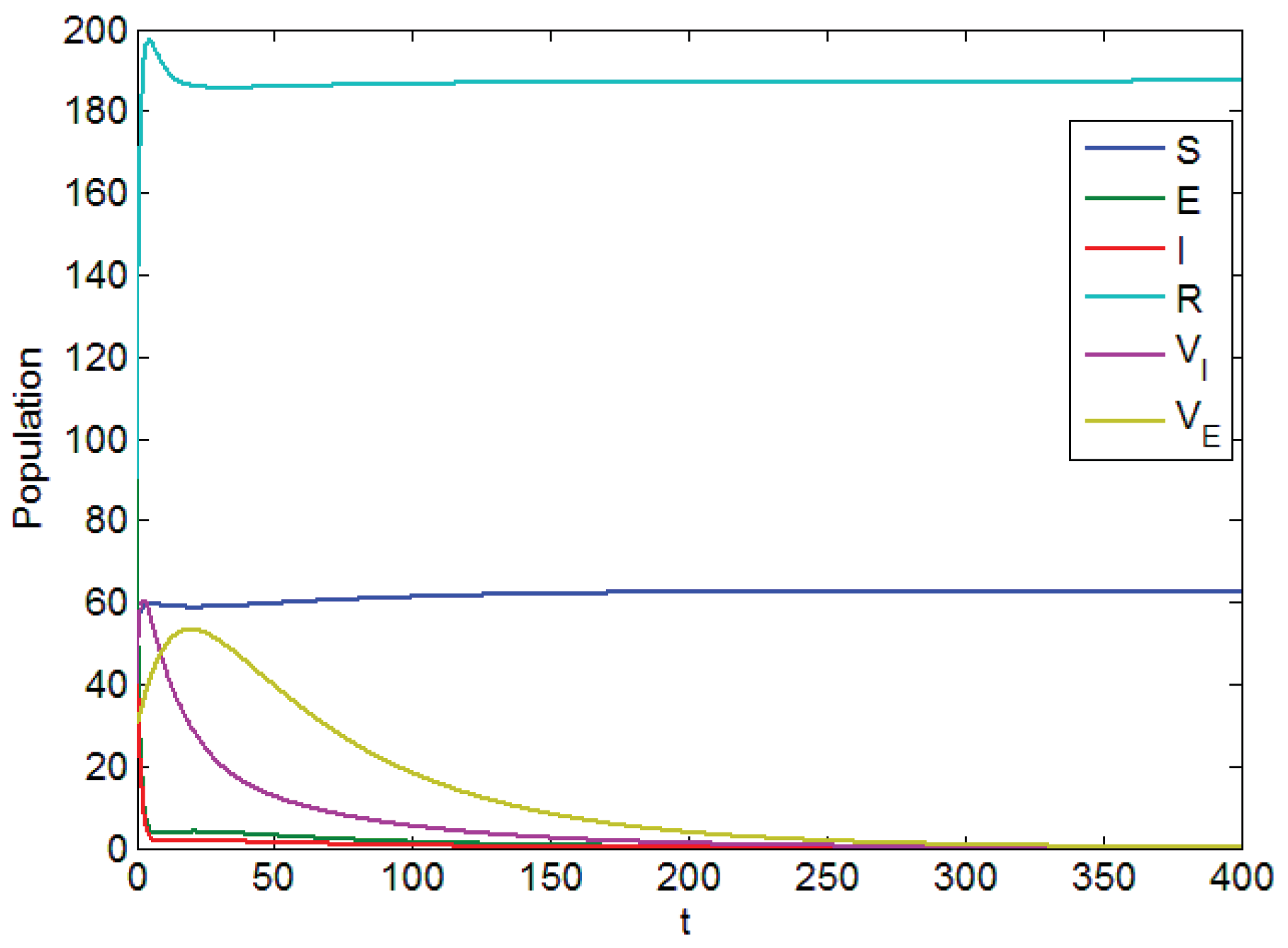
- Using the combination of vaccination and awareness programs only ();Here, v (vaccines) and w (awareness programs) are optimized to obtain the minimum value of the objective function J. Here, let . That is, one supposes that (treatment) here. In Figure 2, one can see that after applying these measures, all populations have their own variations. The susceptible population is decreasing, the exposed population is increasing, the infected population is increasing, and the recovered population is decreasing. Vibrio cholerae is increasing in the human gut as well as in the environment. The basic reproduction number is
- (b)
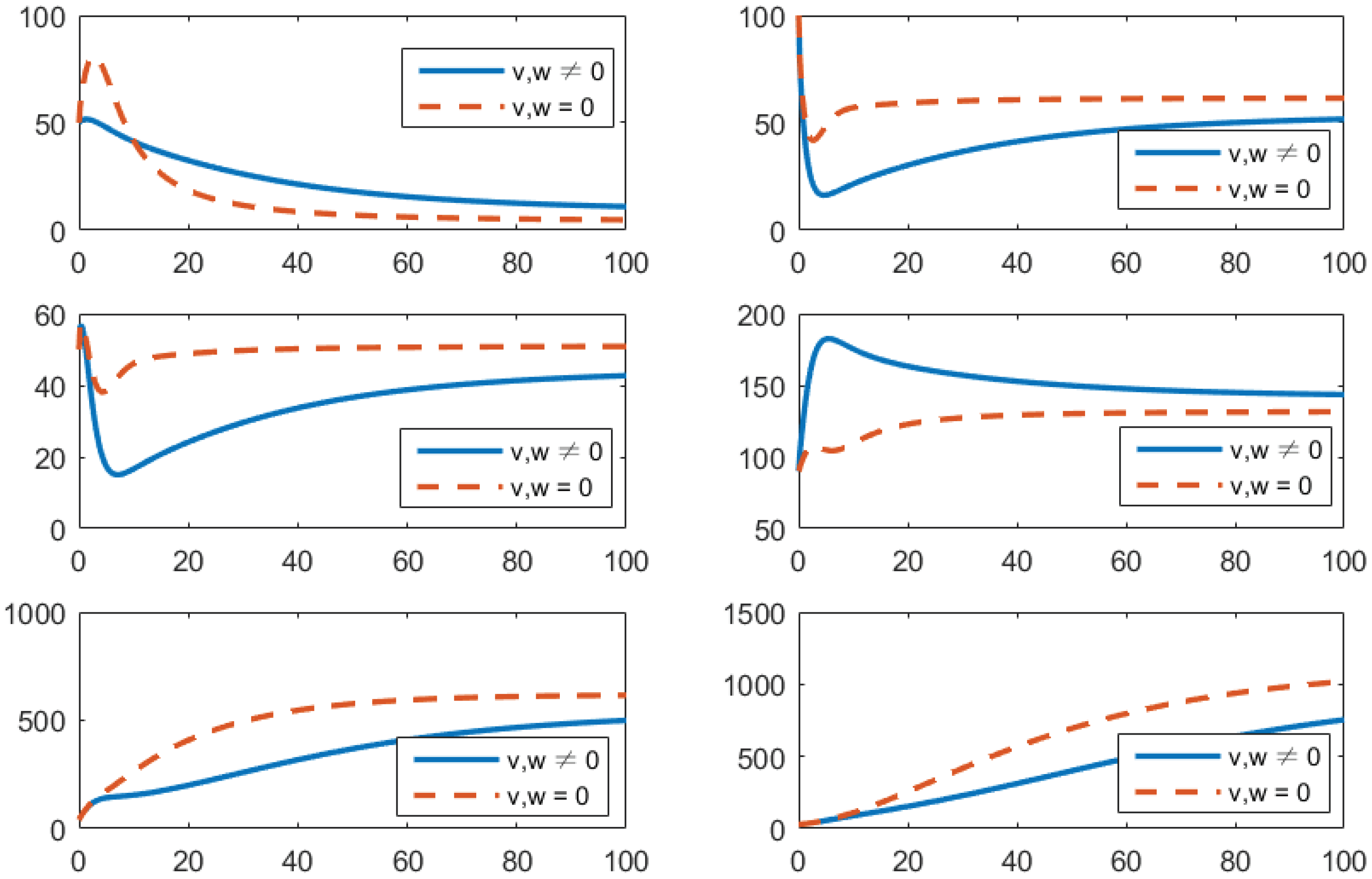
- Using the combination of vaccination and treatment only ();In this strategy, only two controls v (vaccines) and u (treatments) are used to obtain the minimum value of the objective function J. Here, let . That is, one supposes that (awareness programs) here. In Figure 3, one can see that after applying these measures, all populations have their own variations. The susceptible population is increasing, the exposed population is decreasing, the infected population is decreasing, and the recovered population is increasing. Vibrio cholerae is decreasing in the human gut as well as in the environment. The basic reproduction number is
- (c)
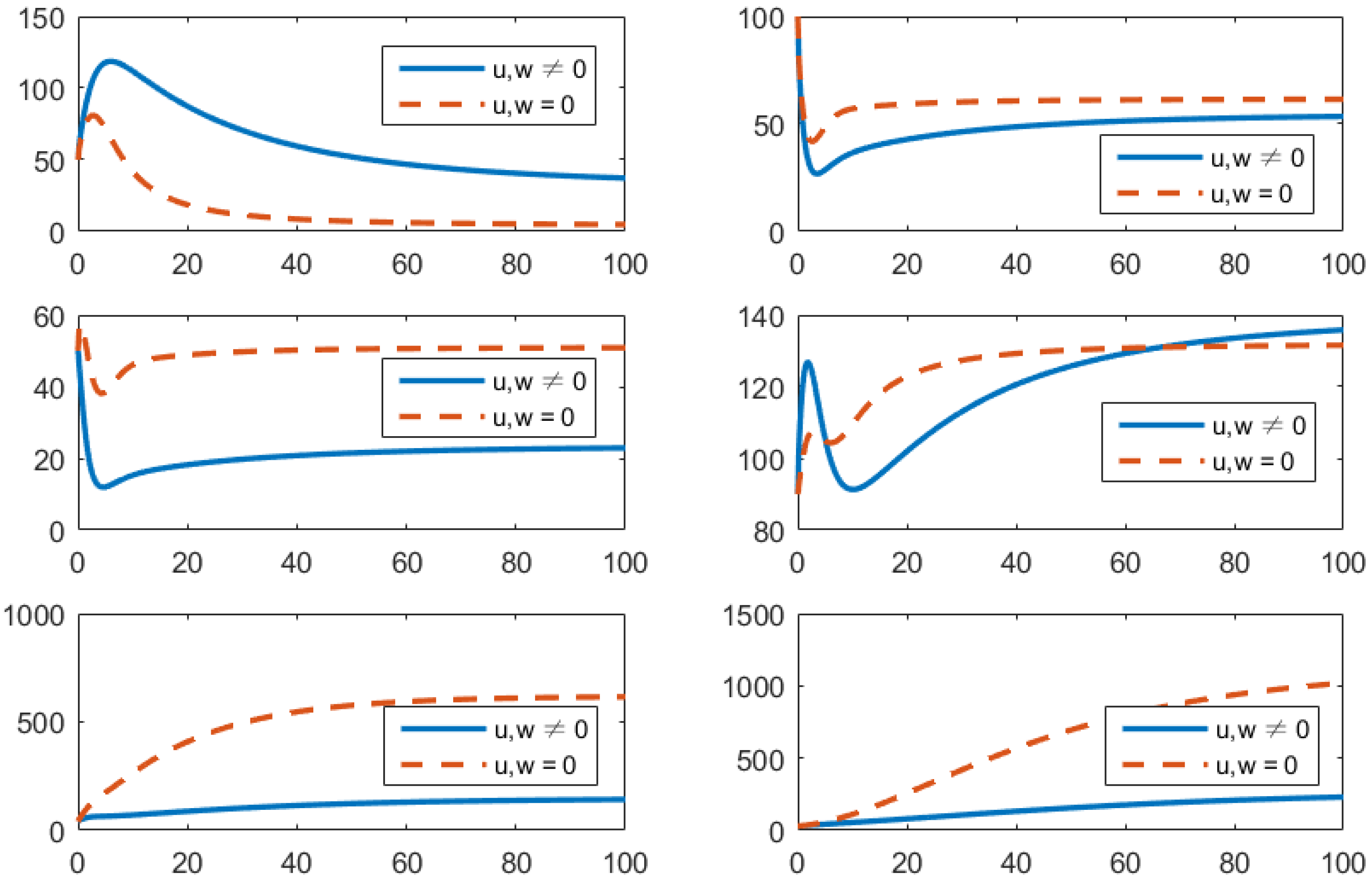
- Using the combination of treatment and awareness programs only ();Here, u (treatments) and w (awareness programs) are optimized to obtain the minimum value of the objective function J. Here, let . That is, one supposes that (vaccines) here. In Figure 4, one can see that after applying these measures, all populations have their own variations. The susceptible population is increasing, the exposed population is decreasing, the infected population is decreasing, and the recovered population is increasing. Vibrio cholerae is decreasing in the human gut as well as in the environment. The basic reproduction number is
- (d)
- Using the combination of treatment, vaccination, and awareness programs ();In this strategy, all controllers u (treatments), v (vaccines), and w (awareness programs) are optimized to obtain the minimum value of the objective function J. Here, let . In Figure 5, one can see that after applying these measures, all populations have their own variations. The susceptible population is increasing, the exposed population is decreasing, the infected population is decreasing, and the recovered population is increasing. Vibrio cholerae is decreasing in the human gut as well as in the environment. The basic reproduction number is
Cost-Effectiveness Analysis
6. Conclusions
Author Contributions
Funding
Institutional Review Board Statement
Informed Consent Statement
Data Availability Statement
Conflicts of Interest
References
- Shuai, Z.; Tien, J.H.; Van den Driessche, P. Cholera Models with Hyperinfectivity and Temporary Immunity. Bull. Math. Biol. 2012, 74, 2423–2445. [Google Scholar] [CrossRef] [PubMed]
- Capasso, V.; Paveri-Fontana, S.L. A Mathematical Model for the 1973 Cholera Epidemic in the European Mediterranean Region. Rev. Epidemiol. Sante Publique 1979, 27, 121–132. [Google Scholar] [PubMed]
- Codeço, C.T. Endemic and Epidemic Dynamics of Cholera: The Role of the Aquatic Reservoir. BMC Infect. Dis. 2001, 1, 1–14. [Google Scholar] [CrossRef] [Green Version]
- Miller Neilan, R.L.; Schaefer, E.; Gaff, H.; Fister, K.R.; Lenhart, S. Modeling Optimal Intervention Strategies for Cholera. Bull. Math. Biol. 2010, 72, 2004–2018. [Google Scholar] [CrossRef]
- Merrell, D.S.; Butler, S.M.; Qadri, F.; Dolganov, N.A.; Alam, A.; Cohen, M.B.; Calderwood, S.B.; Schoolnik, G.K.; Camilli, A. Host-Induced Epidemic Spread of the Cholera Bacterium. Nature 2002, 417, 642–645. [Google Scholar] [CrossRef]
- Joh, R.I.; Wang, H.; Weiss, H.; Weitz, J.S. Dynamics of Indirectly Transmitted Infectious Diseases with Immunological Threshold. Bull. Math. Biol. 2009, 71, 845–862. [Google Scholar] [CrossRef] [Green Version]
- Capone, F.; De Cataldis, V.; De Luca, R. Influence of Diffusion on the Stability of Equilibria in a Reaction-Diffusion System Modeling Cholera Dynamic. J. Math. Biol. 2015, 71, 1107–1131, Erratum in J. Math. Biol. 2015, 71, 1267–1268. [Google Scholar] [CrossRef]
- Podlubny, I. Fractional Differential Equations: An Introduction to Fractional Derivatives, Fractional Differential Equations, to Methods of Their Solution and Some of Their Applications; Academic Press: Cambridge, MA, USA, 1999. [Google Scholar]
- Caputo, M.; Fabrizio, M. A New Definition of Fractional Derivative without Singular Kernel. Progr. Fract. Differ. Appl. 2015, 1, 73–85. [Google Scholar]
- Abdon, A.; Baleanu, D. New Fractional Derivatives with Nonlocal and Non-Singular Kernel: Theory and Application to Heat Transfer Model. Therm. Sci. 2016, 20, 763–769. [Google Scholar]
- Saeedian, M.; Khalighi, M.; Azimi-Tafreshi, N.; Jafari, G.R.; Ausloos, M. Memory Effects on Epidemic Evolution: The Susceptible-Infected-Recovered Epidemic Model. Phys. Rev. E 2017, 95, 22409. [Google Scholar] [CrossRef] [Green Version]
- Rihan, F.A. Numerical Modeling of Fractional-Order Biological Systems. Abstr. Appl. Anal. 2013, 2013, 816803. [Google Scholar] [CrossRef] [Green Version]
- Okyere, E.; Oduro, F.T.; Amponsah, S.K.; Dontwi, I.K. Fractional Order Optimal Control Model for Malaria Infection. arXiv 2016, arXiv:1607.01612. [Google Scholar]
- Yongsheng, D.; Ye, H. A Fractional-Order Differential Equation Model of HIV Infection of CD4+ T-Cells. Math. Comput. Model. 2009, 50, 386–392. [Google Scholar]
- Singh, J.; Kumar, D.; Baleanu, D. On the Analysis of Chemical Kinetics System Pertaining to a Fractional Derivative with Mittag-Leffler Type Kernel. Chaos 2017, 27, 103113. [Google Scholar] [CrossRef]
- Okyere, E.; Oduro, F.T.; Amponsah, S.K.; Dontwi, I.K.; Frempong, N.K. Fractional Order SIR Model with Constant Population. Br. J. Math. Comput. Sci. 2016, 14, 1–12. [Google Scholar] [CrossRef]
- Sweilam, N.H.; Al-Mekhlafi, S.M.; Baleanu, D. Optimal control for a fractional tuberculosis infection model including the impact of diabetes and resistant strains. J. Adv. Res. 2019, 17, 125–137. [Google Scholar] [CrossRef] [PubMed]
- Bonyah, E.B. Fractional optimal control for a corruption model. J. Prime Res. Math. 2020, 16, 11–29. [Google Scholar]
- Khan, A.; Zarin, R.; Akgül, A.; Saeed, A.; Gul, T. Fractional optimal control of COVID-19 pandemic model with generalized Mittag-Leffler function. Adv. Differ. Equations 2021, 1, 387. [Google Scholar] [CrossRef] [PubMed]
- Anderson, R.M.; May, R.M. Infectious Diseases of Humans: Dynamics and Control; Oxford University Press: Oxford, UK, 1991. [Google Scholar]
- Saha, D.; Karim, M.M.; Khan, W.A.; Ahmed, S.; Salam, M.A.; Bennish, M.L. Single-Dose Azithromycin for the Treatment of Cholera in Adults. N. Engl. J. Med. 2006, 354, 2452–2462. [Google Scholar] [CrossRef] [PubMed] [Green Version]
- Das, J.K.; Ali, A.; Salam, R.A.; Bhutta, Z.A. Antibiotics for the Treatment of Cholera, Shigella and Cryptosporidium in Children. BMC Public Health 2013, 13, S10. [Google Scholar] [CrossRef] [Green Version]
- Yang, C.; Wang, X.; Gao, D.; Wang, J. Impact of Awareness Programs on Cholera Dynamics: Two Modeling Approaches. Bull. Math. Biol. 2017, 79, 2109–2131. [Google Scholar] [CrossRef] [PubMed]
- Okosun, K.O.; Rachid, O.; Marcus, N. Optimal Control Strategies and Cost-Effectiveness Analysis of a Malaria Model. BioSystems 2013, 111, 83–101. [Google Scholar] [CrossRef] [PubMed]
- Mwasa, A.; Tchuenche, J.M. Mathematical Analysis of a Cholera Model with Public Health Interventions. BioSystems 2011, 105, 190–200. [Google Scholar] [CrossRef] [PubMed]
- Panja, P. Optimal Control Analysis of a Cholera Epidemic Model. Biophys. Rev. Lett. 2019, 14, 27–48. [Google Scholar] [CrossRef] [Green Version]
- Eckalbar, J.C.; Eckalbar, W.L. Dynamics of an Epidemic Model with Quadratic Treatment. Nonlinear Anal. Real World Appl. 2011, 12, 320–332. [Google Scholar] [CrossRef]
- Hove-Musekwa, S.D.; Nyabadza, F.; Chiyaka, C.; Das, P.; Tripathi, A.; Mukandavire, Z. Modelling and Analysis of the Effects of Malnutrition in the Spread of Cholera. Math. Comput. Model. 2011, 53, 1583–1595. [Google Scholar] [CrossRef]
- Kar, T.K.; Jana, S. A Theoretical Study on Mathematical Modelling of an Infectious Disease with Application of Optimal Control. BioSystems 2013, 111, 37–50. [Google Scholar] [CrossRef]
- Andrews, J.R.; Basu, S. Transmission Dynamics and Control of Cholera in Haiti: An Epidemic Model. Lancet 2011, 377, 1248–1255. [Google Scholar] [CrossRef] [Green Version]
- Okosun, K.O.; Ouifki, R.; Marcus, N. Optimal Control Analysis of a Malaria Disease Transmission Model That Includes Treatment and Vaccination with Waning Immunity. BioSystems 2011, 106, 136–145. [Google Scholar] [CrossRef]
- Cheng, J.; Liang, L.; Park, J.H.; Yan, H.; Li, K. A Dynamic Event-Triggered Approach to State Estimation for Switched Memristive Neural Networks With Nonhomogeneous Sojourn Probabilities. IEEE Trans. Circuits Syst. Regul. Pap. 2021, 68, 4924–4934. [Google Scholar] [CrossRef]
- Cheng, J.; Park, J.J.H.; Wu, Z.G.; Yan, H. Ultimate boundedness control for networked singularly perturbed systems with deception attacks: A markovian communication protocol approach. IEEE Trans. Netw. Sci. Eng. 2021. [Google Scholar] [CrossRef]
- Xie, L.; Cheng, J.; Wang, H.; Wang, J.; Hu, M.; Zhou, Z. Memory-based event-triggered asynchronous control for semi-Markov switching systems. Appl. Math. Comput. 2022, 415, 126694. [Google Scholar] [CrossRef]


| Parameter | Estimated Value | Parameter | Estimated Value |
|---|---|---|---|
| 0.73 [28] | A | 50 day [29] | |
| 0.01 [26] | a | 0.6 [30] | |
| 0.6 [26] | 6 cell per infected human [26] | ||
| 0.001 [4] | 0.2 [29] | ||
| 0.52 [30] | 1/30 day [28] | ||
| 2.3 [30] | 2$ per infected person [4] | ||
| 0.52 [30] | 6$ per person [4] | ||
| m | 0.005 [30] | 1$ per person [26] |
| Strategies | Number of Infections Avoided | Total Costs | ICER |
|---|---|---|---|
| Uncontrolled | 0 | 0 | 0 |
| 198.69 | 17,705.2659 | 89.11 | |
| 243.15 | 18,561.1209 | 19.25 | |
| 353.28 | 8769.2521 | −88.9119 | |
| 475.189 | 24,893.2485 | 132.2626 |
| Strategies | Number of Infections Avoided | Total Costs | ICER |
|---|---|---|---|
| 243.15 | 18,561.1209 | 19.25 | |
| 353.28 | 8769.2521 | −88.9119 | |
| 475.189 | 24,893.2485 | 132.2626 |
| Strategies | Number of Infections Avoided | Total Costs | ICER |
|---|---|---|---|
| 353.28 | 8769.2521 | −88.9119 | |
| 475.189 | 24,893.2485 | 132.2626 |
Publisher’s Note: MDPI stays neutral with regard to jurisdictional claims in published maps and institutional affiliations. |
© 2022 by the authors. Licensee MDPI, Basel, Switzerland. This article is an open access article distributed under the terms and conditions of the Creative Commons Attribution (CC BY) license (https://creativecommons.org/licenses/by/4.0/).
Share and Cite
He, Y.; Wang, Z. Stability Analysis and Optimal Control of a Fractional Cholera Epidemic Model. Fractal Fract. 2022, 6, 157. https://doi.org/10.3390/fractalfract6030157
He Y, Wang Z. Stability Analysis and Optimal Control of a Fractional Cholera Epidemic Model. Fractal and Fractional. 2022; 6(3):157. https://doi.org/10.3390/fractalfract6030157
Chicago/Turabian StyleHe, Yanyan, and Zhen Wang. 2022. "Stability Analysis and Optimal Control of a Fractional Cholera Epidemic Model" Fractal and Fractional 6, no. 3: 157. https://doi.org/10.3390/fractalfract6030157
APA StyleHe, Y., & Wang, Z. (2022). Stability Analysis and Optimal Control of a Fractional Cholera Epidemic Model. Fractal and Fractional, 6(3), 157. https://doi.org/10.3390/fractalfract6030157