
Numerical Algorithm for Calculating the Time Domain Response of Fractional Order Transfer Function


Abstract
1. Introduction
2. Definition
3. The Numerical Algorithm for EFOTF
4. The Numerical Algorithm for IFOTF
4.1. Numerical Convolution
4.2. Numerical Inversion of Convolution
5. Error Analysis
6. Calculation Examples
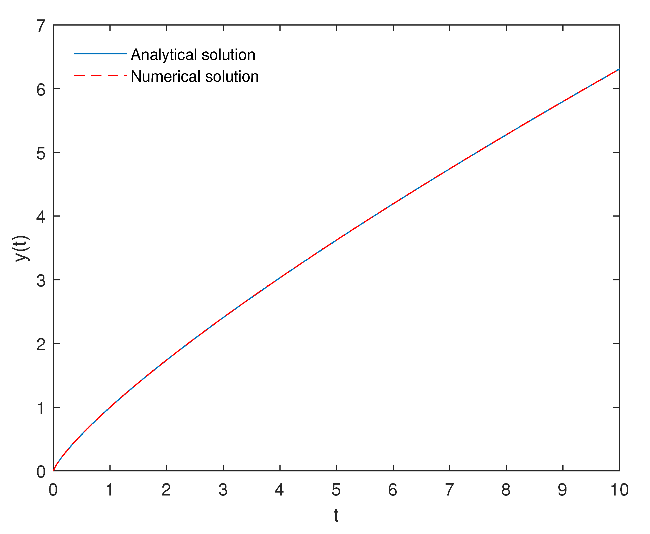
6.1. Example 1
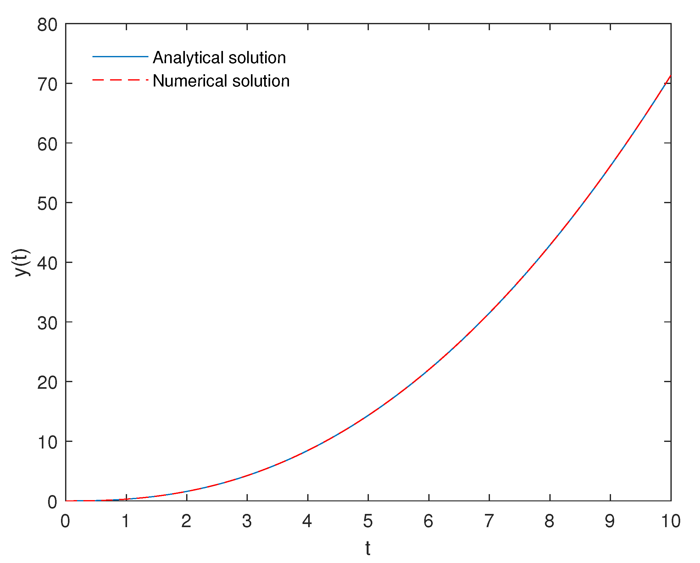
6.2. Example 2
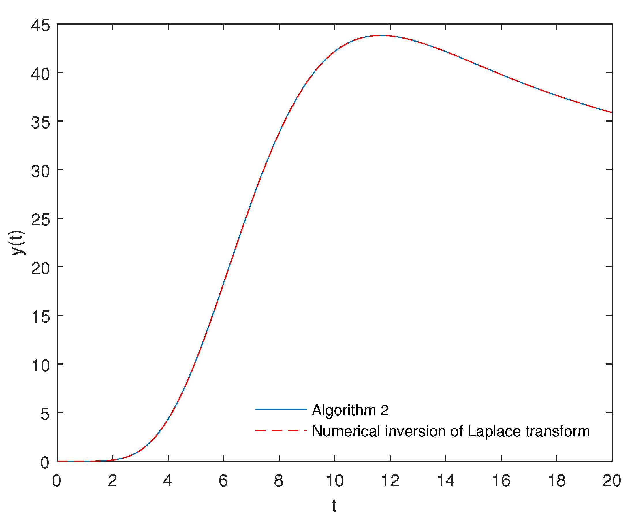
6.3. Example 3
6.4. Example 4
7. Discussion
Author Contributions
Funding
Data Availability Statement
Conflicts of Interest
References
- Liu, B.; Su, H.S.; Wu, L.C.; Li, X.L.; Lu, X. Fractional-order controllability of multi-agent systems with time-delay. Neurocomputing 2021, 424, 268–277. [Google Scholar] [CrossRef]
- Ahmad, I.; Rahman, G.U.; Ahmad, S.; Alshehri, N.A.; Elagan, S.K. Controllability of a damped nonlinear fractional order integrodifferential system with input delay. Alex. Eng. J. 2022, 61, 1956–1966. [Google Scholar] [CrossRef]
- Shamardan, A.B.; Moubarak, M.R.A. Controllability and observability for fractional control systems. J. Fract. Calc. 1999, 15, 25–34. [Google Scholar]
- Hassanzadeh, I.; Tabatabaei, M. Calculation of controllability and observability matrices for special case of continuous-time multi-order fractional systems. ISA Trans. 2018, 82, 62–72. [Google Scholar] [CrossRef]
- Zhang, X.F.; Zhao, Z.L. Normalization and stabilization for rectangular singular fractional order T-S fuzzy systems. Fuzzy Sets Syst. 2020, 381, 140–153. [Google Scholar] [CrossRef]
- Zhang, X.F. Relationship between integer order systems and fractional order systems and its two applications. IEEE-CAA J. Autom. Sin. 2018, 5, 639–643. [Google Scholar] [CrossRef]
- Zhang, X.F.; Chen, Y.Q. Admissibility and robust stabilization of continuous linear singular fractional order systems with the fractional order α: The 0 < α < 1 case. ISA Trans. 2018, 82, 42–50. [Google Scholar]
- Chen, Y.Q.; Ahn, H.S.; Xue, D.Y. Robust controllability of interval fractional order linear time invariant systems. Signal Process. 2006, 86, 2794–2802. [Google Scholar] [CrossRef]
- Zhang, J.X.; Yang, G.H. Robust Adaptive Fault-Tolerant Control for a Class of Unknown Nonlinear Systems. IEEE Trans. Ind. Electron. 2017, 64, 585–594. [Google Scholar] [CrossRef]
- Zhang, X.F.; Huang, W.K. Adaptive neural network sliding mode control for nonlinear singular fractional order systems with mismatched uncertainties. Fractal Fract. 2020, 4, 50. [Google Scholar] [CrossRef]
- Zhang, J.X.; Yang, G.H. Low-complexity tracking control of strict-feedback systems with unknown control directions. IEEE Trans. Autom. Control 2019, 64, 5175–5182. [Google Scholar] [CrossRef]
- Zhang, J.X.; Yang, G.H. Fuzzy adaptive output feedback control of uncertain nonlinear systems with prescribed performance. IEEE Trans. Cybern. 2018, 48, 1342–1354. [Google Scholar] [CrossRef]
- Mandić, P.D.; Šekara, T.B.; Lazarević, M.P.; Bošković, M. Dominant pole placement with fractional order PID controllers: D-decomposition approach. ISA Trans. 2017, 67, 76–86. [Google Scholar] [CrossRef]
- Mandić, P.D.; Lazarević, M.P.; Šekara, T.B. D-Decomposition technique for stabilization of furuta pendulum: Fractional approach. Bull. Pol. Acad. Sci. Tech. Sci. 2016, 64, 189–196. [Google Scholar] [CrossRef][Green Version]
- Krijnen, M.E.; van Ostayen, R.; HosseinNia, S.H. The application of fractional order control for an air-based contactless actuation system. ISA Trans. 2018, 82, 172–183. [Google Scholar] [CrossRef]
- Marinangeli, L.; Alijani, F.; HosseinNia, S.H. Fractional-order positive position feedback compensator for active vibration control of a smart composite plate. J. Sound Vib. 2018, 412, 1–16. [Google Scholar] [CrossRef]
- Yang, Y.; Xue, D.Y. A novel actual load forecasting by interval grey modeling methodology based on the fractional calculus. ISA Trans. 2018, 82, 200–209. [Google Scholar] [CrossRef]
- Yang, Y.; Xue, D.Y. Continuous fractional-order grey model and electricity prediction research based on the observation error feedback. Energy 2016, 115, 722–733. [Google Scholar] [CrossRef]
- Sun, H.G.; Yong, Z.; Baleanu, D.; Chen, W.; Chen, Y.Q. A new collection of real world applications of fractional calculus in science and engineering. Commun. Nonlinear Sci. Numer. Simul. 2018, 64, 213–231. [Google Scholar] [CrossRef]
- Lubich, C. On the stability of linear multistep methods for Volterra convolution equations. IMA J. Numer. Anal. 1983, 3, 439–465. [Google Scholar] [CrossRef]
- Lubich, C. Discretized fractional calculus. SIAM J. Math. Anal. 1986, 17, 704–719. [Google Scholar] [CrossRef]
- Lubich, C. Fractional linear multistep methods for Abel-Volterra integral equations of the first kind. IMA J. Numer. Anal. 1987, 7, 97–106. [Google Scholar] [CrossRef]
- Daftardar-Gejji, V.; Bhalekara, S. Boundary value problems for multi-term fractional differential equations. J. Math. Anal. Appl. 2008, 345, 754–765. [Google Scholar] [CrossRef]
- Diethelm, K.; Ford, N.J.; Freed, A.D. A predictor-corrector approach for the numerical solution of fractional differential equations. Nonlinear Dyn. 2002, 29, 3–22. [Google Scholar] [CrossRef]
- Diethelm, K. An investigation of some nonclassical methods for the numerical approximation of Caputo-type fractional derivatives. Numer. Algorithms 2008, 47, 361–390. [Google Scholar] [CrossRef]
- Diethelm, K. The Analysis of Fractional Differential Equations; Springer: Berlin, Germany, 2010; pp. 229–248. [Google Scholar]
- Podlubny, I. Matrix approach to discrete fractional calculus. Fract. Calc. Appl. Anal. 2000, 3, 359–386. [Google Scholar]
- Wei, Y.Q.; Liu, D.Y.; Driss, B.; Chen, Y.M. An improved pseudo-state estimator for a class of commensurate fractional order linear systems based on fractional order modulating functions. Syst. Control. Lett. 2018, 118, 29–34. [Google Scholar] [CrossRef]
- Chen, Y.M.; Liu, L.Q.; Liu, D.Y.; Boutat, D. Numerical study of a class of variable order nonlinear fractional differential equation in terms of Bernstein polynomials. Ain Shams Eng. J. 2018, 9, 1235–1241. [Google Scholar] [CrossRef]
- Liu, D.Y.; Tian, Y.; Boutat, D.; Laleg-Kirati, T. An algebraic fractional order differentiator for a class of signals satisfying a linear differential equation. Signal Process. 2015, 116, 78–90. [Google Scholar] [CrossRef]
- Xue, D.Y. Fractional-Order Control Systems-Fundamentals and Numerical Implementations; De Gruyter: Berlin, Germany, 2017; pp. 1–30. [Google Scholar]
- Mansouri, R.; Bettayeb, M.; Djennoune, S. Approximating of high order integer systems by fractional order reduced parameter models. Math. Comput. Model. 2010, 51, 53–62. [Google Scholar] [CrossRef]
- Caponetto, R.; Dongola, G.; Fortuna, L.; Graziani, S.; Strazzeri, S. A fractional model for IPMC actuators. In Proceedings of the 2008 IEEE Instrumentation and Measurement Technology Conference, Victoria, BC, Canada, 20 June 2008. [Google Scholar]
- Caponetto, R.; Graziani, S.; Pappalardo, F.; Umana, E.; Xibilia, M.G.; Giamberardino, P. A scalable fractional order model for IPMC actuators. IFAC Proc. Vol. 2012, 45, 593–596. [Google Scholar] [CrossRef]
- Caponetto, R.; Graziani, S.; Pappalardo, F.; Xibilia, M.G. Parametric Control of IPMC Actuator Modeled as Fractional Order System. Adv. Sci. Technol. 2013, 79, 63–68. [Google Scholar]
- Podlubny, I. Fractional Differential Equations: An Introduction to Fractional Derivatives, Fractional Differential Equations, to Methods of Their Solution and Some of Their Applications; Academic Press: Cambridge, MA, USA, 1998; pp. 41–119. [Google Scholar]
- Caputo, M. Linear Models of dissipation whose Q is almost frequency independent. Geophys. J. R. Astr. Soc. 1967, 13, 529–539. [Google Scholar] [CrossRef]
- Brualdi, R.A. Introductory Combinatorics, 5th ed.; Pearson Education: New York, NY, USA, 2009; pp. 127–160. [Google Scholar]
- Xue, D.Y.; Bai, L. Numerical algorithms for Caputo fractional-order differential equations. Int. J. Control 2017, 90, 1201–1211. [Google Scholar] [CrossRef]
- Sabatier, J.; Farges, C. Analysis of fractional models physical consistency. J. Vib. Control 2017, 23, 895–908. [Google Scholar] [CrossRef]
- Valsa, J.; Brancik, L. Approximate formulae for numerical inversion of Laplace transforms. Int. J. Numer. Model. 1998, 11, 153–166. [Google Scholar] [CrossRef]


| Step Size | |||||
|---|---|---|---|---|---|
| Standard PECE-Type Adams Algorithm | Algorithm 1 | |||
|---|---|---|---|---|
| Step Size | Maximal Error | Execution Time | Maximal Error | Execution Time |
| 0.3904 | 101.2 s | 0.01250 | 0.35667 s | |
| 0.2193 | 368.4 s | 0.00681 | 0.43396 s | |
| 0.1164 | 1358.0 s | 0.00358 | 0.99232 s | |
| 0.0600 | 5017.4 s | 0.00185 | 2.54765 s | |
| Step Size | |||||
|---|---|---|---|---|---|
| Step Size | |||||
|---|---|---|---|---|---|
Publisher’s Note: MDPI stays neutral with regard to jurisdictional claims in published maps and institutional affiliations. |
© 2022 by the authors. Licensee MDPI, Basel, Switzerland. This article is an open access article distributed under the terms and conditions of the Creative Commons Attribution (CC BY) license (https://creativecommons.org/licenses/by/4.0/).
Share and Cite
Bai, L.; Xue, D. Numerical Algorithm for Calculating the Time Domain Response of Fractional Order Transfer Function. Fractal Fract. 2022, 6, 122. https://doi.org/10.3390/fractalfract6020122
Bai L, Xue D. Numerical Algorithm for Calculating the Time Domain Response of Fractional Order Transfer Function. Fractal and Fractional. 2022; 6(2):122. https://doi.org/10.3390/fractalfract6020122
Chicago/Turabian StyleBai, Lu, and Dingyü Xue. 2022. "Numerical Algorithm for Calculating the Time Domain Response of Fractional Order Transfer Function" Fractal and Fractional 6, no. 2: 122. https://doi.org/10.3390/fractalfract6020122
APA StyleBai, L., & Xue, D. (2022). Numerical Algorithm for Calculating the Time Domain Response of Fractional Order Transfer Function. Fractal and Fractional, 6(2), 122. https://doi.org/10.3390/fractalfract6020122