Abstract
Unconventional shale reservoirs and typical fine-grained rocks exhibit complicated, oriented features at various scales. Due to the complex geometry, combination and arrangement of grains, as well as the substantial heterogeneity of shale, it is challenging to analyze the oriented structures of shale accurately. In this study, we propose a model that combines both multifractal and structural entropy theory to determine the oriented structures of shale. First, we perform FE–SEM experiments to specify the microstructural characteristics of shale. Next, the shape, size and orientation parameters of the grains and pores are identified via image processing. Then fractal dimensions of grain flatness, grain alignment and pore orientation are calculated and substituted into the structural entropy equation to obtain the structure-oriented entropy model. Lastly, the proposed model is applied to study the orientation characteristic of the Yan-Chang #7 Shale Formation in Ordos Basin, China. A total of 1470 SEM images of 20 shale samples is analyzed to calculate the structure-oriented entropy (SOE) of Yan-Chang #7 Shale, whose values range from 0.78 to 0.96. The grains exhibit directional arrangement (SOE ≥ 0.85) but are randomly distributed (SOE < 0.85). Calculations of samples with different compositions show that clay and organic matters are two major governing factors for the directivity of shale. The grain alignment pattern diagram analyses reveal three types of orientation structures: fusiform, spider-like and eggette-like. The proposed model can quantitatively evaluate the oriented structure of shale, which helps better understand the intrinsic characteristics of shale and thereby assists the successful exploitation of shale resources.
1. Introduction
The shale reservoirs play a critical role in exploring and exploiting unconventional hydrocarbon resources due to their large reserves, proven to be 2.2073 × 10¹⁴ m3 [1]. In 2018, shale gas production in the United States reached about 6.7 × 10¹¹ m3, accounting for 63.4% of the total produced natural gas and altering the global natural gas supply pattern [2]. In China, gigantic shale resource reserves have been discovered and distributed in Bohai Bay, Ordos, Sichuan and Songliao Basins [3,4].
The shale rocks are featured with high heterogeneity, low permeability (0.0001~0.1 mD) and porosity (1~6%) [5,6,7]. The shale grains possess complex geometry, combination and arrangement, which exhibit a laminated structure, layer couple structure and directional alignment of grains at the macroscale, mesoscale and microscale. The microstructures of shale, including orientation, arrangement and spatial distribution of the grains, are fundamental properties that determine the mechanical properties (i.e., Young’s modulus, Poisson’s ratio and breakage strength) of shale. Meanwhile, shales exhibiting the oriented structure characteristics are more susceptible to developing new fractures in response to external forces. The pivotal petrophysical properties, including porosity, pore throat connectivity and permeability, are also affected by the orientation and arrangement of grains. Quantitatively evaluating the orientated structures of shale can help to discover geological and engineering sweet spots and aid in the design of shale reservoir drilling and fracturing. However, we currently lack a mathematical model to quantitatively determine the oriented structure characteristics of shale due to the substantial heterogeneity and complicated arrangement of grains [8,9].
Many scholars have extensively investigated the microstructure of sedimentary rock by examining the characteristics of grains and pores. Previous studies have employed various visualization techniques, including the X-ray diffraction method, polarizing microscopy, high-resolution electron microscopy and transmission electron microscopy techniques [10]. The X-ray diffraction method is applied to measure the parallelism or randomness of the grain based on the intensity of basal reflections [11]. Gillott et al. (1970) proposed a “structural index” to indicate the grain orientation, which was defined as the areal ratio between the diffraction peaks in the parallel orientation plane of vertical grains and that of parallel grains [12]. Due to the limited detecting scope (maximum observation area is about 5.56 μm × 5.56 μm), the X-ray diffraction method and polarizing microscopes are gradually replaced by transmission electron microscopy techniques [13]. Previous studies provided a descriptive or semi-quantitative description to analyze the oriented structure properties of shale, which could only obtain the microstructure of rock within a narrow area [14]. Visual characterizations of shale, capturing the microstructure characteristics and reducing the heterogeneity impact, are needed to better understand shale’s orientation features.
Fractal theory can simplify the features of the objects by evaluating their intricate structure, which has been applied in various fields, such as aggregate characterization [15], complex network analysis [16,17], shape recognition [18], pore structure analyses [19,20] and texture segmentation [21]. Wu (1988) first used entropy to characterize the clay microstructure and concluded that entropy could be utilized as a quantitative parameter to examine the structural arrangement of clay [22]. Liu et al. (1992) proposed a grain-size fractal dimension to survey the heterogeneity of grain [23]. Xie et al. (1997) proposed structural potential to describe the association and arrangement of the rock grain, providing a quantitative characterization of the microstructure features of clay [24]. Xia et al. (2021) implemented the fractal parameters to analyze the microstructure of porous media and then examine the correlations between calculated fractal dimensions and permeability [25]. Zhu et al. (2022) established a three-dimensional model to investigate the complexities of the fracture network in the formation by multifractal methods [26]. Li et al. (2022) proposed a box-counting fractal dimension method for evaluating the pore structure complexity of digital rocks [27]. The previous results prove that fractal dimension is a feasible and effective way to characterize the complex pore structures of rock. However, the orientation features of shale can be affected by the size, shape and arrangement of grains and the type, amount and distribution of pores, which cannot be quantified by one fractal dimension.
In this study, we propose a model to quantitatively determine the oriented structures of shale by combining the structural orientation entropy and multifractal theory. First, the FE–SEM and image stitching techniques were applied to obtain the microstructure characteristics of shale over a relatively large scope (84 μm × 84 μm). Then image processing was conducted by ImageJ software to obtain the size, orientation, perimeter and shape parameters of grains and pores. Next, based on the statistics of pores and grains, we calculated the representative fractal dimensions and then screened out the ones pertaining to the orientation to formulate the structure entropy model. The coefficients of the proposed model were obtained by fitting the permeability data of samples with different degrees of orientation. Lastly, the proposed model was applied to determine the orientation characteristics, investigate the influential factors and specify the directivity patterns of the Yan-Chang #7 Shale Formation.
2. Geological Settings
2.1. Geological Background
The Ordos Basin is located in the middle of China with an area of 32 × 104 km2 across the Shannxi, Gansu, Ningxia, Neimenggu and Shanxi Provinces [28]. Six structural units, including the Yimeng uplift, Weibel uplift, Tianhuan depression, thrust belt, Jinxi fold belt and Yishan slope, are found in the Ordos Basin [29]. The Ordos Basin has undergone three crucial stages of tectonic movement, the late Caledonian, late Indosinian and late Yanshan [3].
Shale possesses complex geometry, combination and arrangement of grains, which exhibit laminated structure, layer couple structure and directional alignment of grains at the macroscale, mesoscale and microscale. In Figure 1, one shale outcrop (located in the southern Ordos Basin)—which exhibits laminated structures with interlayered distributions of light and dark layers from decimeters to meter scales—is depicted. We then retrieve two samples (A and B) from this outcrop to investigate their microstructure characteristics by FE–SEM characterization. Those results are also shown in Figure 1. Sample A’s grains are arranged randomly, while sample B’s grains are distributed in a particular direction. Despite these two samples sharing a similar layered structure at the macroscale, their grain alignment characteristics differ significantly at the microscale. The structure characteristics obtained at the macroscale cannot be directly applied to the microscale. Given that the pores and fractures govern shale gas flow in the matrix at micro/nanoscales, it is important to determine the oriented microstructures of shale.
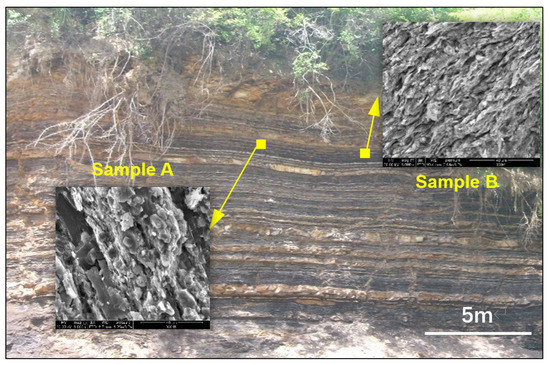
Figure 1.
Outcrop showing where samples A and B are retrieved and the SEM results of these two samples.
2.2. Sampling Location
Thirty-five shale samples were collected from twenty-five drilling wells and eight outcrops in the Yan-Chang #7 Shale Formation of the Ordos Basin. The locations of drilling wells and outcrops where the samples were retrieved are depicted in Figure 2. The downhole core samples were drilled from wells at the Fuxian, Qingyang, Zhengning and Dingbian areas, while the outcrop samples were collected from eight well-preserved shale outcrops in the southern Ordos Basin.
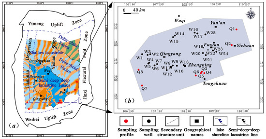
Figure 2.
Geological and geographic background of the studied area: (a) the structural subdivisions and sedimentary facies of the Ordos Basin; (b) wells and outcrops showing where the samples were retrieved.
The outcrop, full-diameter core and standard core in the Yan-Chang #7 Formation of the Ordos Basin are illustrated in Figure 3. The representative shale outcrops (Q6, Q7) of the Yan-Chang #7 Shale Formation are depicted in Figure 3a,b. The Q6 outcrop is the typical “Zhangjiatan” shale, which formed in a deep-lake and semi-deep-lake sedimentary environment and exhibited high organic matter content (1.26~34.41%) as well as layer structure characteristics [30,31]. Besides, the outcrop Q7 consists of dark or gray-black and silt mixed shale, exhibiting layered structures with a thickness of 20 m. The shale samples retrieved from the outcrop Q7 with an apparent layered structure characteristic are shown in Figure 3c. The full diameter (a diameter of 100 mm, a height of 120 mm) and standard cores (a diameter of 25.4 mm, a height of 50 mm) of the Yan-Chang #7 Shale Formation are illustrated in Figure 3d–f.
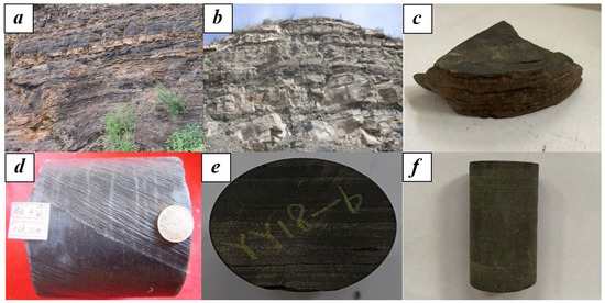
Figure 3.
The outcrops, full diameter and standard cores retrieved from the Yan-Chang #7 Shale Formation of the Ordos Basin. (a) Q6, outcrops, surface; (b) Q7, outcrops, surface; (c) #S35, sample from outcrop, surface; (d) #S20, full-diameter core sample, downhole 1028.72 m; (e,f) #S9, standard core sample, downhole 1448.79 m.
3. Structure Entropy Model
As depicted in Figure 1, the shale rocks exhibit complicated directional features. To quantitatively determine the oriented structures of shale, we propose a structure entropy model composed of multiple fractal dimensions to characterize the microstructure characteristics comprehensively. Fractal dimensions sensitive to the directivity of shale were evaluated and then screened to formulate an integrated oriented-structure entropy (SOE) model. The FE–SEM characterization and image stitching were used to obtain the microstructure parameters for calculating the fractal dimensions over a relatively large scope. The coefficients of the proposed SOE model were determined by fitting the permeability data of samples with different degrees of directivity.
3.1. Oriented-Structure Entropy Model
Entropy provides an analytical tool for examining complicated systems since it statistically measures the disorder of a system [32]. During sedimentation, the microstructure characteristics of shale (orientation, arrangement and spatial distribution of the shale grain) continuously change, resulting in the alteration of the entropy values. Hence, the calculated entropy values can be used to estimate the disorder of grain arrangement and orientation at the microscale.
Wu (1988) proposed a structure entropy model to quantitatively investigate the oriented features of rock structure, which is formulated as follows [22]:
where SS is the structure entropy; Sa and Sg are entropy of grain arrangement and size, respectively.
Geometrically, the oriented structure characteristics of shale are primarily manifested in two aspects: the arrangement relationships of shale grains and their distribution [33]. However, the spreading organic pores are formed by the dissolution or decomposition of kerogen, independent of the grain alignment. Also, the organic pores are in nanoscales, whose size plays a role in structure entropy calculation. Thus, the SOE model of shale considers the structural characteristics of both grains and pores, expressed as:
where S is the structure entropy; subscripts ga, gs and pa represent grain alignment, size and pore arrangement, respectively.
3.2. Fractal Dimension Selection for the Entropy Model
Previous studies have shown that fractal dimensions (FD) can be used to approximate the structure entropy [24]. To screen out the suitable fractal dimensions, we first selected nine representative fractal dimensions that can reflect the oriented microstructures of shale. Next, FE–SEM characterization and image processing were introduced to show how to obtain the fundamental properties used in the FD calculations. Then the nine FDs of samples with different degrees of directivity were calculated. Lastly, based on the variations of FD values, we selected the ones sensitive to the sample’s directivity.
3.2.1. FE–SEM Characterization and Image Processing
The Quanta FEI 450 FE–SEM instrument (FEI Company) was applied to acquire the microstructure characteristics of shale samples. Before the measurement, the samples were polished with argon ion beams and then coated with gold.
The pores and fractures are in micro/nanoscales in shale, which can be detected under a large magnification and result in limited observation windows [34]. Due to the heterogeneity, complexity and randomness of grains’ arrangement and orientation, one or several FE–SEM images cannot obtain the sample’s comprehensive microstructure characteristics. Hence, we used an image stitching technique to form a large SEM image that can maintain the detailed pore structure information and reduce the effect of heterogeneity. The stitched image was composed of 7 × 7 SEM images, reflecting the microscopic details over 84 μm × 84 μm.
Based on the stitched images, image processing software (ImageJ) was applied to identify the shape, size and orientation parameters of the grains and pores of shale samples. The stitched FE–SEM image and the ones after processing are depicted in Figure 4. The detailed procedures of the image processing are:
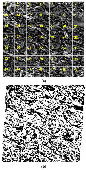
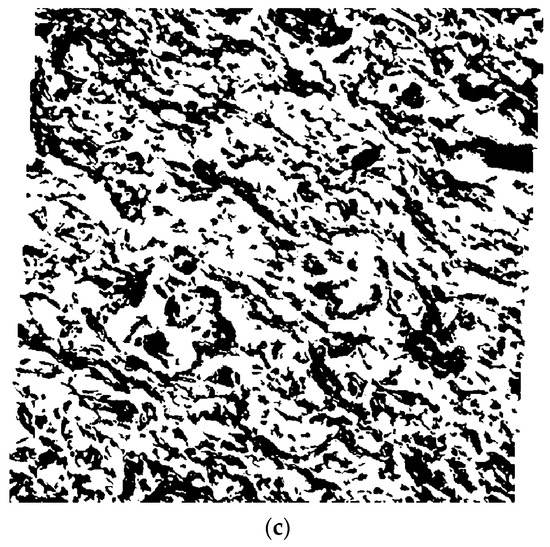
Figure 4.
Illustrations of (a) stitched FE–SEM images; (b) grayscale images obtained by ImageJ; and (c) noise-reduced grayscale images.
- Grayscale conversion. The FE–SEM images of the shale samples were first transformed into 8-bit grayscale images.
- Grayscale threshold selection. The threshold values of the images can be tuned to display the morphologies of grains and pores. In this study, the threshold values of grains and pores are in the range of 0–73 and 88–255, respectively. The FE–SEM image showing the morphologies of grains is illustrated in Figure 4b. The black area represents grains, while the white ones stand for pores.
- Image noise reduction. After threshold processing, many noise spots are shown in the images, affecting the processing accuracy. The image after noise reduction is illustrated in Figure 4c.
ImageJ and the stitched SEM images were used to obtain the parameters for characterizing the pore structures of shale samples, summarized in Table 1. The pore and grains treated are ellipses; the long and short axis of the ellipse, as well as the ratio, dip angle and perimeter of pores and grains, are statistically analyzed.

Table 1.
The parameters used to determine pores and grains’ structure characteristics.
3.2.2. Fractal Dimension Calculation
Nine FDs related to the alignment of grains and pores, the size of grains and pores, and the distribution of grains and pores were selected. The mathematic formulas and parameters used in the calculations are summarized in Table 2. To screen out the FDs that are sensitive to the oriented structures of pore structures, we built two conceptual models with different degrees of directivity, as shown in Figure 5. Both the grains and pores are distributed randomly for sample #1, while a clear directivity is shown in sample #2. Based on the abovementioned image processing procedures and equations of FDs, we calculated the nine FDs of these two conceptual models. Their values are listed in Table 3.
Table 2.
The mathematic formulas and corresponding parameters of the selected nine FDs.
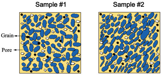
Figure 5.
Conceptual shale samples with different degrees of directivity.
Table 3.
The calculated nine FDs of two conceptual models with different degrees of directivity.
The calculated results demonstrate that the fractal dimensions of grain flatness, pore flatness, pore size, grain size distribution, pore size distribution and surface roughness values of these samples are similar; their difference is within 2.15%. However, the variations of fractal dimensions of grain orientation, pore orientation and grain size range from 6.28% to 7.46%, which are significantly higher than others. The sensitivity analyses of fractal dimensions are consistent with the entropy evaluation, jointly proving that the fractal dimensions of grain alignment, grain size and pore distribution can reflect the directivity of the sample. In Figure A1 in Appendix B, the straight line of the graph of fractal dimensions of grain alignment, grain size and pore distribution demonstrate how fractal dimensions are obtained.
3.2.3. Oriented-Structure Entropy Model
Wu (1988) used a linear polynomial structure entropy model to quantify the structure’s characteristics of clay [22]. The coefficients all equal the unit in the model, which requires further examination before applying it to other scenarios. Adopting this liner function and FDs’ sensitivity to directivity, we propose the oriented-structure entropy of shale as:
where DGO is the fractal dimension of grain orientation; DPO is the fractal dimension of pore orientation; DGS is the fractal dimension of grain size; and A, B and C are coefficients.
At similar pore size and connectivity conditions, samples with a higher degree of directivity exhibit large permeability, especially when the flow direction coincides with the orientation of the pore structure. Previous studies also demonstrated a strong correlation between the layered features of shale and permeability [25]. We first prepared a synthetic core sample based on the typical composition of the Yan-Chang #7 shale formation. Next, the proposed characterization procedures were applied to obtain the FDs of the artificial core sample. Then the gas permeabilities of the samples were measured by core flooding experiments. Lastly, the permeability data and the evaluated SOE values were used to calculate the coefficients in the model.
The synthetic core samples were composed of quartz, feldspar, smectite, illite, kaolinite powders and isolated kerogen. The size of mineral powders ranged from 1000 mesh to 6000 mesh, while the kerogen powders possessed larger sizes but exhibited low content (<10 wt%). A synthetic shale sample can be obtained by the process of interfusion, stuffing and compaction; the detailed procedures for preparing an artificial shale sample can be found in [35,36]. The synthetic shale samples #G1–#G10 are shown in Figure 6. The white arrow indicates the direction of the laminated shale. The prepared core samples are first subjected to radial core flooding experiments and then cut into small pieces for FE–SEM measurements and the microsection test.
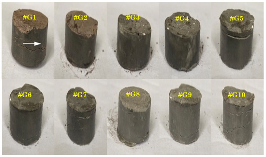
Figure 6.
Photos of synthetic shale core samples #G1–#G10. The white arrow in the Figure 6 stands for the direction of the oriented structures of the synthetic shale core samples.
The direction of permeability measurement and the location of the plug used in FE–SEM characterization are depicted in Figure 7. The especially radial core flooding experiments measure the permeability parallel to the orientation of the synthetic core sample. The coating face of the plug shows the detailed features of the laminated structure.
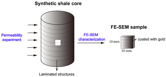
Figure 7.
The schematic diagram showing the direction of permeability measurement and location of the plug for the FE–SEM experiment.
Transverse permeability tests are utilized to measure the permeability of synthetic shale core samples. On cylindrical core samples, radial flow tests are performed rather than axial flow tests. This technique is based on creating an infinite reservoir condition by simply keeping the upstream pressure constant. Afterward, a pressure pulse is created by reducing the pressure in the downstream reservoir. Permeability of the test sample is ultimately determined by interpreting pressure buildup data collected by the pressure transducer in the downstream. The radial permeability of shale samples can be calculated as follows:
where K is the core porosity; kφ is the concentration diffusion coefficient of rock pores; M is the molar mass of helium; μ is the average viscosity of the inlet end and the outlet end; φ is the core porosity; z is the helium density under the pressure of p; ρ is the helium density under the pressure of p0; R is the ideal gas constant equal to 8.314 J/(mol K); and T is the temperature.
Based on the image processing results, we then calculated the DGO, DPO and DGS. The SOE is evaluated by initially assuming the coefficients equal to 1/3. Consequently, a smaller value of SOE indicates a higher degree of directivity. We also assumed the SOE value is between 0 and 1, representing the microstructure of shale exhibiting completely random distribution and perfectly oriented structures, respectively. The calculated DGO, DPO and DGS and measured permeabilities of these core samples are listed in Table 4. Then the coefficients A, B and C are tuned to fit the permeability data; the ones that exhibit the largest determination of coefficient (R2 = 0.9995) are used in the model. The fitted coefficient for DGO, DPO and DGS is 0.278, 0.396 and 0.325, respectively. Therefore, the SOE is defined as:
Table 4.
The fractal dimensions and permeability of the synthetic core samples.
3.2.4. Model Verification
Shale possesses complex geometry, combination and arrangement of grains, which exhibits layer, layer couple and directional alignment at the macroscale, mesoscale and microscale, respectively. Typically, the greater the degree of oriented structures at the microscale, the more developed the layer structure of shale at the macroscale. To verify the accuracy of the SOE model, the SOE value was compared to the stratification density (numbers of layers in unit length). In this study, the stratification density of shale samples can be calculated by the microsection test. The schematic of stratification density, showing how the stratification density of shale can be determined by microsection, is demonstrated in Figure 8. We calculated the stratification densities of 10 synthetic shale core samples (#G1–#G10) to analyze the association with SOE values. In addition, the samples that can be used to conduct the microsection test were consistent with those used for the FE–SEM technique, which helped to minimize the impact of shale heterogeneities.
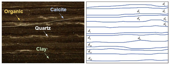
Figure 8.
The microsection of synthetic sample #G1 and the corresponding schematic of stratification density.
The SOE values and the stratification densities of 10 synthetic shale core samples are compared in Figure 9. The results show that a negative correlation exists in the SOE values and stratification densities with the R2 of 0.7343. The relation indicates that the SOE model provides a credible estimate for the oriented structure properties of shale.
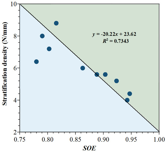
Figure 9.
Parity chart of the SOE values and stratification densities of 10 synthetic shale core samples.
4. Results and Discussions
In this section, the Yan-Chang #7 shale formation is used to exemplify the application of the proposed SOE model. The FE–SEM characterization was first conducted to obtain the parameters for FDs calculations. Then the SOE values of 20 samples were evaluated, and their directivity patterns were specified. Lastly, the relationships between SOE values and mineral compositions were established.
4.1. Sample Compositions
Due to the strong heterogeneity of shale, samples with different composition exhibit distinct pore structure characteristics. The mineral composition and TOC content of shale samples were identified by X-ray diffraction (D8 ADVANCE) experiment and carbon-sulfur analyzer (CS230 SH), respectively. The box diagram of mineral compositions and histograms of TOC contents of shale samples are displayed in Figure 10. The results show that shale samples contain detrital minerals (quartz and feldspar), carbonate minerals (calcite, dolomite and Gypsum) and clay minerals (illite, smectite, chlorite, kaolinite, illite-smectite mixed layer), as depicted in Figure 10a. The TOC contents of shale samples range between 0.71 and 36.76%, with 73% of samples possessing TOC contents greater than 2%, as shown in Figure 10b. The detailed mineral composition, TOC, and Ro are summarized in Table A1 in Appendix A.
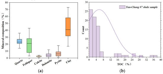
Figure 10.
Diagrams of (a) mineral composition and (b) TOC content of samples retrieved from Yan-Chang #7 Shale Formation in the Ordos Basin.
Based on the mineral composition and TOC content, the shale samples can be divided into five types: (1) low-TOC clayey shale (LC); (2) high- TOC clayey shale (HC); (3) low- TOC sandy shale (LS); (4) high- TOC sandy shale (HS); and (5) low-TOC mixed shale (LS), as shown in Figure 11. The division between high and low TOC content refers to the Oil and Gas Industry Standards (GB/T31483-2015) of the People’s Republic of China.
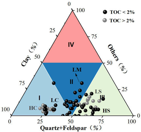
Figure 11.
The ternary diagram showing the five types of shale retrieved from Yan-Chang #7 Shale Formation in the Ordos Basin.
4.2. FE–SEM Characterization
Twenty shale samples’ oriented micro-structure characteristics were investigated by FE–SEM characterization. The SEM images of the five classified types of shale are summarized in Figure 12. Samples #S21, #S41, #S33, #S52 and #S63 belong to high-TOC clayey shale, high-TOC sandy shale, low-TOC clayey shale, low-TOC mixed shale and low-TOC sandy shale, respectively. The FE–SEM images revealed the differences in grain orientation, grain type and contact of each type of shale. Three types of contacts, edge-to-edge contact (EE), edge-to-face contact (EF) and face-to-face contact (FF), were identified in the obtained SEM images, as shown in Figure 12a [33]. The face-to-face contact of parallel bundles of clay flakes, frequently observed in the high-TOC clayey shale and resulting in a high degree of directivity, is illustrated in Figure 12b. In Figure 12c, the edge-to-face contact between clay grains and flakes, noted in the high-TOC sandy shale and exhibiting a moderate degree of directivity, is depicted. The edge-to-face contacts are identified in the low-TOC sandy shale and low-TOC clayey shale; no directivity of these two types of shale is shown in Figure 12d,e. The clay and silt edges are connected in the low-TOC mixed shale, forming a cellular structure and demonstrating no clear directivity, as shown in Figure 12f.
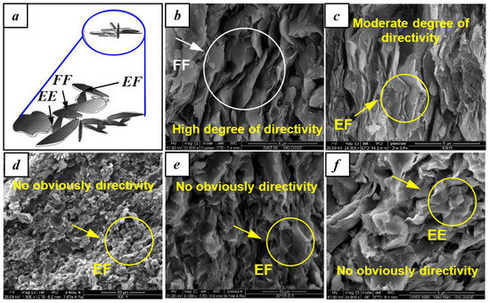
Figure 12.
FE–SEM images of five different types of downhole shale samples. (a) The schematic diagram showing the different contact manners of grains [31]; (b) high-TOC clayey shale, #S21, 784.24 m; (c) high-TOC sandy shale, #S41, 1448.79 m; (d) low-TOC clayey shale, #S33, 1071.83 m; (e) low-TOC mixed shale, #S52, 1151.32 m; (f) low-TOC sandy shale, #S63, 1448.79 m.
Because various orientation features can be observed in the heterogeneous shale sample, the visual analyses are performed on the stitched SEM images. A total of 1470 FE–SEM images of 20 samples were obtained; 44,331 grains and 43,430 pores were identified by image processing and used to calculate the SOE values. The stitched FE–SEM images and those after noise reduction of all the samples are summarized in Table A2. Due to the minor deviations during the continuous shift of FE–SEM characterization, the stitched images are in the shape of a parallelogram. The average parameters characterizing the dimension, shape and size of grains and pores for evaluating the microstructure characteristics of shale, respectively, are listed in Table A3 and Table A4. The probability distribution functions, expressions and determination coefficients of these parameters are summarized in Table 5. The obtained size and perimeter of grains and pores data follow the Gaussian distribution, while the flatness of grains and pore data obeys the Lorentz function.
Table 5.
Probability distribution functions, expressions and determination coefficients of size, perimeter and flatness of grains and pores.
4.3. Oriented Structure Characteristics of Shale
4.3.1. Multifractal and SOE
To quantitatively evaluate the oriented structure characteristics of shale samples, we calculated the multifractals and SOE values, respectively. The obtained DGO, DPO, DGS and SOE values of 20 shale samples are listed in Table 6. The DGO, DPO, DGS and SOE values of Yan-Chang #7 Shale are in the range of 0.781–0.991, 0.771–0.991, 0.792–0.956 and 0.780–0.968, respectively.
Table 6.
The calculated DGO, DPO, DGS and SOE values of 20 shale samples.
The box plots of SOE and DGO, DPO and DGS values of five types of shale are shown in Figure 13. The error bar in the plot refers to the maximum and minimum of the evaluated parameter, while the box indicates the upper and lower quartiles of the data. The ranges of SOE values for high-TOC clayey shale, high-TOC sandy shale, low-TOC clayey shale, low-TOC sandy shale and low-TOC mixed shale are 0.781–0.947, 0.892–0.933, 0.867–0.931, 0.921–0.966 and 0.942–0.968 with average values of 0.868, 0.917, 0.903, 0.948 and 0.959, respectively. Among the tested shale samples, the high-TOC clayey shales have the lowest SOE values, which indicates well-oriented structures and echoes well with the previous FE–SEM results. The high-TOC sandy shale and low-TOC clayey shale possess similar SOE values, while the low-TOC mixed shale and low-TOC sandy shales share comparable SOE values.
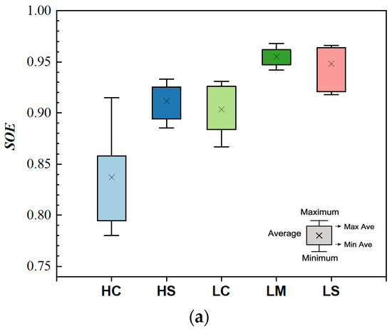
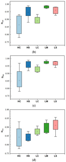
Figure 13.
The box plots of (a) SOE and (b) DGO, (c) DPO and (d) DGS values of five types of shale in the Yan-Chang #7 Shale Formation of the Ordos Basin.
To distinguish the differences in microstructure among the four types of shale, we compare the values of DGO, DPO and DGS, as shown in Figure 13b–d, respectively. Results show that the high-TOC sandy shales have a smaller DGS, suggesting that the high-TOC sandy shale has well-sorted grains. Similar observations have been found by Lu et al. (2023) [37]. The high-TOC sandy shales are typically deposited in a shallow lake environment characterized by deep water, a low energy regime and a slow accumulation rate [38]. The mineral grains formed in this sedimentation stage are relatively homogeneous. Besides, results also show that the DGO and DGS of the low-TOC clayey shale are smaller than those of the high-TOC sandy shale, low-TOC mixed shale and low-TOC sandy shale, leading to the low-TOC clayey shale having a good degree of directivity and sorted grain size. The DGO, DPO and DGS of the low-TOC mixed shale and low-TOC sandy shale are more significant than that of other types of shale, indicating that the grains and pores are randomly distributed and poorly sorted.
Previous studies have indicated that the oriented structures of shale are governed by both the depositional environment and diagenesis [31]. The initial grain size distribution is determined by the accumulation rate, the energy regime and the physicochemical properties of water during the deposition period, which can be represented by DGS in the SOE model. Additionally, the grain alignment could alter in response to overburden stress, tectonic stress and overpressure of hydrocarbon evolution.
4.3.2. The Influential Factors of SOE
Based on the obtained SOE values and the compositions of the samples, we then examined the impacts of TOC and mineral composition on the oriented structures. In Figure A1 in Appendix B, the correlations between TOC/mineral composition and the SOE values are summarized. The obtained correlations and R2 are listed in Table 7. The results show that the SOE values correlate with the clay mineral and TOC contents, whose R2s are 0.7559 and 0.6379, respectively. However, the SOEs are independent of the quartz (R2 = 0.0392), feldspar (R2 = 0.2231), calcite (R2 = 0.0816), dolomite (R2 = 0.0843) and pyrite (R2 = 0.1181). Larger clay and TOC contents of shale result in more noticeable oriented structures of shale. The Yan-Chang #7 Shales, possessing high clay and moderate TOC contents, are typically deposited in semi-deep–deep lake conditions [38], which helps the development of laminated shale.
Table 7.
Coefficients of determination between TOC/mineral composition and SOE values of shale samples.
4.4. Directivity Patterns of Shale
The above results suggest that the SOE model can be used to quantify the degrees of directivity; however, the detailed directions and directivity patterns of the oriented structures remain unknown. The stitched FE–SEM images of samples #S9, #S50 and #S63, whose SOE values are 0.968, 0.963 and 0.966, respectively, are shown in Figure 14. Despite the similar SOE values, the directivity patterns of these samples are quite different. The grain alignment diagram (rose diagram for grain orientation) is used to specify the direction and pattern of the oriented structure of shale. The grain alignment patterns diagram consists of 72 sector charts, with each sector covering 2.5°. The angle of each sector is the dip angle between the maximum diameter of the shale grain and the horizontal plane, while the length of the sector chart reflects the grain numbers. The pore orientation is affected by the grain arrangement and their contact relations, which lead to the pore orientation being comparable to the grains. Consequently, the pore alignment patterns are not included in this study. The obtained grain alignment diagrams are also shown in Figure 14; the grain alignment diagrams of 20 representative shale samples are summarized in Figure A2.
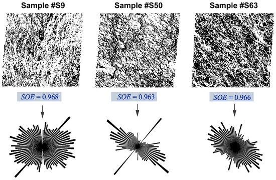
Figure 14.
FE–SEM images and corresponding grain alignment pattern diagrams of samples #S9, #S50 and #S63.
The grain alignment pattern diagrams of 20 shale samples, which can be divided into two groups by their SOE values, are depicted in Figure 15. The samples exhibit noticeable directivity when the SOE values are smaller than 0.85, while the sample shows low degrees of directivity or random distributions when the SOE values are higher than 0.85. We then further investigated the directivity characteristics of the samples based on the patterns of the grain alignment diagrams.
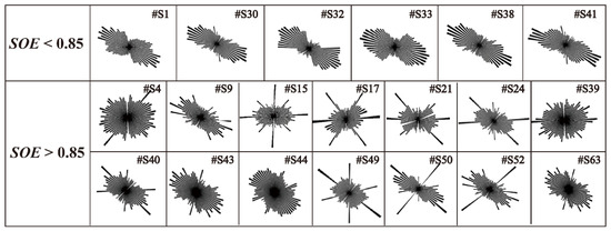
Figure 15.
The grain alignment pattern diagrams of 20 shale samples separated into two groups by their SOE values.
The identified three types of directivity patterns are shown in Figure 16: pattern #1 (fusiform-like shape), pattern #2 (spider-like shape) and pattern #3 (eggette-like shape). Pattern #1 is characterized by a degree of directivity, resulting in fusiform-like shapes. Pattern #2 describes the samples as partially oriented; several sectors exhibit directivity, while most of the sectors are randomly distributed with spider-like shapes. Pattern #3 refers to the grains being completely, randomly distributed and exhibiting an eggette-like directivity pattern.
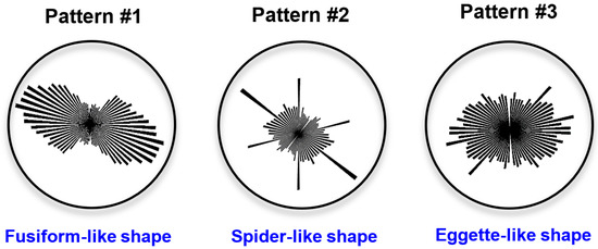
Figure 16.
Three patterns of the grain alignment diagrams: type #1 (fusiform-like shape), type #2 (spider-like shape) and type #3 (eggette-like shape).
We further investigated the grain alignment patterns of five types of shale, as shown in Figure 17. The grains in the high-TOC clayey shale exhibited noticeable orientation structures, belonging to the oriented shape (pattern #1). As for the low-TOC clayey shale, high-TOC sandy shale and low-TOC sandy shale, most of the sectors of the preferred orientation diagram showed no evident directional characteristics. In contrast, several (less than four) sectors exhibited different directions comparing other sectors, which can be classified as the oriented shape (pattern #1) or partially oriented shape (pattern #2). The low-TOC mixed shale demonstrated directivity patterns #2 and #3, whose grains are partially oriented or randomly distributed.
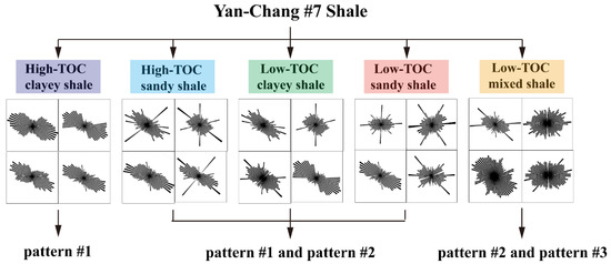
Figure 17.
The grain alignment pattern diagrams that correspond to each type of shale in the Yan-Chang #7 Formation.
5. Conclusions
In this study, we propose a quantitative model to evaluate the oriented structure characteristics of shale at the microscale by combining the stitching FE–SEM images approach, structure entropy and fractal theory. The Yan-Chang #7 Shales in the Ordos basin, China, were employed as a case study to exemplify the application of the model; the obtained oriented structure characteristics were classified and analyzed. The following conclusions can be drawn:
- Based on many FE–SEM characterizations, the fractal dimensions of grain orientation, the fractal dimension of pore orientation and the fractal dimension of grain size were selected to form the oriented structure entropy model. The synthetic cores were prepared, and their permeabilities are measured to determine the coefficients in the SOE model.
- The SOE model is applied to evaluate the oriented structures of Yan-Chang #7 Shale; the obtained SOE values are in the range of 0.780–0.968. The threshold value of SOE for the samples to exhibit directional features is 0.85; samples with SOEs larger than 0.85 demonstrate the random distribution of grains.
- The TOC and clay minerals are the crucial factors that affect the oriented structures of shale. The SOE values are both strongly correlated with the clay mineral and TOC contents with R2s of 0.7559 and 0.6379, respectively, but poorly related with other minerals.
- Grain alignment patterns can be classified as pattern #1 (fusiform-like shape), pattern #2 (spider-like shape) and pattern #3 (eggette-like shape). High-TOC clayey shales show the typical pattern #1 grain alignment. Low-TOC clayey shale, high-TOC sandy shale and low-TOC sandy shale have the characteristics of both patterns #1 and #2. The grain alignment of low-TOC mixed shales belongs to patterns #2 and #3.
Author Contributions
Conceptualization and funding acquisition, X.X. and H.D.; methodology and writing—review and editing, L.H.; software, R.L.; validation, Y.L. and X.X.; formal analysis and data curation, J.M. All authors have read and agreed to the published version of the manuscript.
Funding
This study is funded by Sichuan Innovation Seedling Project [No: 80303-AMZ023] to the first author (Xie. X.) and National Natural Science Foundation of China [No: 42072182] to the corresponding author (Deng. H.). We gratefully acknowledge this support.
Data Availability Statement
The data corresponding to the figures generated in this review can be obtained upon request to the author.
Conflicts of Interest
The authors declare no conflict of interest.
Appendix A
Table A1.
The mineral composition and TOC content of Yan-Chang #7 Shales include both outcrops and drilled cores.
Table A1.
The mineral composition and TOC content of Yan-Chang #7 Shales include both outcrops and drilled cores.
| Sample No. | Well Site | Formation | Depth (m) | Mineral Content (%) | TOC (%) | Ro (%) | Organic Type | ||||||
|---|---|---|---|---|---|---|---|---|---|---|---|---|---|
| Quartz | Feldspar | Calcite | Dolomite | Pyrite | Gypsum | Clay | |||||||
| #S1 | Q1 | Chang #7 | Outcrop | 26 | 29 | 0 | 0 | 0 | 0 | 45 | 5.17 | - | II1 |
| #S2 | Q1 | Chang #7 | Outcrop | 19 | 23 | 0 | 0 | 0 | 0 | 58 | 2.61 | - | II2 |
| #S3 | Q2 | Chang #7 | Outcrop | 32 | 33 | 3 | 2 | 0 | 0 | 30 | 1.26 | - | I |
| #S4 | Q3 | Chang #7 | Outcrop | 33 | 5 | 1 | 3 | 25 | 3 | 33 | 2.08 | - | II2 |
| #S5 | Q3 | Chang #7 | Outcrop | 47 | 4 | 2 | 1 | 17 | 0 | 29 | 29.34 | - | II1 |
| #S6 | Q3 | Chang #7 | Outcrop | 62 | 6 | 6 | 0 | 0 | 0 | 26 | 24.44 | - | II1 |
| #S7 | Q3 | Chang #7 | Outcrop | 22 | 25 | 3 | 5 | 10 | 3 | 35 | 2.25 | - | II1 |
| #S8 | Q4 | Chang #7 | Outcrop | 35 | 31 | 0 | 0 | 0 | 0 | 34 | 18.41 | - | II1 |
| #S9 | Q5 | Chang #7 | Outcrop | 25 | 16 | 1 | 2 | 22 | 1 | 34 | 1.96 | - | II1 |
| #S10 | Q5 | Chang #7 | Outcrop | 23 | 18 | 1 | 1 | 20 | 0 | 37 | 2.49 | - | II2 |
| #S11 | Q5 | Chang #7 | Outcrop | 58 | 8 | 5 | 0 | 2 | 0 | 28 | 21.49 | - | II2 |
| #S12 | Q5 | Chang #7 | Outcrop | 18 | 26 | 4 | 2 | 18 | 0 | 32 | 2.40 | - | I |
| #S13 | Q5 | Chang #7 | Outcrop | 26 | 29 | 4 | 2 | 15 | 0 | 24 | 24.78 | - | II1 |
| #S14 | Q6 | Chang #7 | Outcrop | 23 | 29 | 0 | 0 | 0 | 0 | 48 | 16.07 | - | II1 |
| #S15 | Q7 | Chang #7 | Outcrop | 31 | 30 | 0 | 0 | 0 | 0 | 39 | 0.78 | - | II1 |
| #S16 | Q8 | Chang #7 | Outcrop | 27 | 18 | 0 | 0 | 0 | 0 | 54 | 34.41 | - | II1 |
| #S17 | W1 | Chang #7 | 768.23 | 23 | 4 | 0 | 2 | 2 | 0 | 70 | 6.45 | - | II1 |
| #S18 | W2 | Chang #7 | 770.70 | 26 | 5 | 0 | 3 | 3 | 0 | 63 | 5.11 | 1.12 | II1 |
| #S19 | W2 | Chang #7 | 727.20 | 26 | 6 | 0 | 4 | 0 | 0 | 63 | 0.71 | 1.07 | II1 |
| #S20 | W2 | Chang #7 | 773.79 | 18 | 7 | 0 | 4 | 0 | 0 | 69 | 3.21 | 0.78 | I |
| #S21 | W2 | Chang #7 | 784.24 | 20 | 3 | 0 | 2 | 7 | 0 | 68 | 14.10 | 1.12 | I |
| #S22 | W2 | Chang #7 | 787.45 | 34 | 4 | 2 | 6 | 6 | 0 | 48 | 5.21 | 1.06 | II1 |
| #S23 | W3 | Chang #7 | 790.14 | 39 | 7 | 0 | 1 | 1 | 0 | 51 | 4.73 | 0.92 | II1 |
| #S24 | W4 | Chang #7 | 1224.04 | 36 | 18 | 2 | 6 | 4 | 0 | 42 | 17.03 | - | II1 |
| #S25 | W5 | Chang #7 | 1263.38 | 23 | 8 | 2 | 8 | 0 | 0 | 59 | 36.76 | - | II1 |
| #S26 | W5 | Chang #7 | 1276.32 | 16 | 6 | 2 | 6 | 0 | 0 | 70 | 0.85 | 1.20 | - |
| #S27 | W5 | Chang #7 | 1280.60 | 22 | 8 | 2 | 4 | 0 | 0 | 63 | 1.05 | 0.88 | - |
| #S28 | W5 | Chang #7 | 1239.70 | 21 | 8 | 2 | 4 | 0 | 0 | 65 | 0.99 | 1.30 | II1 |
| #S29 | W6 | Chang #7 | 1433.37 | 30 | 18 | 4 | 2 | 14 | 0 | 32 | 2.03 | - | II1 |
| #S30 | W6 | Chang #7 | 1435.34 | 22 | 10 | 2 | 5 | 0 | 0 | 62 | 2.51 | 0.72 | II1 |
| #S31 | W6 | Chang #7 | 1436.01 | 19 | 5 | 2 | 5 | 0 | 0 | 70 | 3.53 | 0.75 | II1 |
| #S32 | W6 | Chang #7 | 1437.88 | 20 | 6 | 2 | 5 | 0 | 0 | 67 | 1.13 | 1.12 | II1 |
| #S33 | W6 | Chang #7 | 1071.83 | 18 | 9 | 0 | 4 | 0 | 0 | 69 | 0.93 | 1.17 | II1 |
| #S34 | W7 | Chang #7 | 1084.49 | 16 | 5 | 0 | 7 | 2 | 0 | 69 | 1.24 | 0.83 | II1 |
| #S35 | W7 | Chang #7 | 1087.60 | 17 | 9 | 3 | 4 | 0 | 0 | 68 | 1.52 | 0.83 | - |
| #S36 | W7 | Chang #7 | 1912.09 | 19 | 5 | 1 | 2 | 0 | 0 | 72 | 1.29 | 0.87 | II2 |
| #S37 | W7 | Chang #7 | 1916.66 | 14 | 6 | 2 | 5 | 0 | 0 | 73 | 1.34 | 1.30 | - |
| #S38 | W7 | Chang #7 | 1919.04 | 19 | 6 | 2 | 4 | 0 | 0 | 70 | 0.79 | 1.02 | - |
| #S39 | W8 | Chang #7 | 1924.60 | 47 | 18 | 2 | 9 | 0 | 0 | 32 | 2.51 | - | II1 |
| #S40 | W8 | Chang #7 | 1921.50 | 7 | 12 | 1 | 2 | 28 | 0 | 50 | 3.24 | - | II1 |
| #S41 | W9 | Chang #7 | 1448.79 | 50 | 15 | 2 | 1 | 0 | 0 | 32 | 15.20 | - | II1 |
| #S42 | W10 | Chang #7 | 1450.75 | 25 | 35 | 5 | 9 | 0 | 0 | 26 | 1.31 | - | II1 |
| #S43 | W11 | Chang #7 | 1453.96 | 29 | 26 | 0 | 6 | 9 | 0 | 30 | 1.12 | - | II1 |
| #S44 | W12 | Chang #7 | 1439.60 | 22 | 43 | 2 | 9 | 3 | 0 | 21 | 1.24 | - | II1 |
| #S45 | W13 | Chang #7 | 1495.65 | 28 | 27 | 0 | 12 | 4 | 0 | 29 | 1.54 | - | II1 |
| #S46 | W13 | Chang #7 | 1497.79 | 21 | 20 | 15 | 18 | 2 | 0 | 24 | 0.79 | 1.01 | II2 |
| #S47 | W14 | Chang #7 | 1499.31 | 22 | 24 | 3 | 0 | 4 | 0 | 47 | 3.96 | 1.30 | II2 |
| #S48 | W15 | Chang #7 | 1396.04 | 20 | 22 | 3 | 3 | 7 | 0 | 45 | 5.62 | - | II2 |
| #S49 | W16 | Chang #7 | 1397.62 | 23 | 27 | 3 | 2 | 6 | 0 | 39 | 1.23 | - | II2 |
| #S50 | W17 | Chang #7 | 1399.10 | 25 | 40 | 2 | 0 | 6 | 0 | 27 | 1.32 | - | II1 |
| #S51 | W18 | Chang #7 | 1254.31 | 29 | 35 | 0 | 0 | 6 | 0 | 30 | 5.47 | 1.20 | II1 |
| #S52 | W19 | Chang #7 | 1151.32 | 22 | 27 | 3 | 2 | 5 | 0 | 41 | 4.37 | - | II1 |
| #S53 | W19 | Chang #7 | 1152.48 | 24 | 14 | 2 | 3 | 6 | 0 | 51 | 2.59 | - | II1 |
| #S54 | W19 | Chang #7 | 1188.03 | 24 | 37 | 2 | 0 | 6 | 0 | 31 | 3.24 | 1.26 | II1 |
| #S55 | W19 | Chang #7 | 1189.25 | 23 | 38 | 2 | 0 | 6 | 0 | 31 | 4.74 | - | II1 |
| #S56 | W19 | Chang #7 | 1220.21 | 30 | 28 | 3 | 0 | 2 | 0 | 37 | 2.94 | 1.08 | II2 |
| #S57 | W19 | Chang #7 | 1224.04 | 26 | 28 | 0 | 0 | 4 | 0 | 42 | 2.35 | 1.16 | II2 |
| #S58 | W19 | Chang #7 | 1263.38 | 23 | 22 | 2 | 2 | 8 | 0 | 43 | 4.21 | - | II2 |
| #S59 | W19 | Chang #7 | 1276.32 | 23 | 25 | 3 | 2 | 6 | 0 | 41 | 2.08 | 1.11 | II2 |
| #S60 | W19 | Chang #7 | 1280.60 | 26 | 27 | 3 | 3 | 3 | 0 | 38 | 2.51 | - | II2 |
| #S61 | W19 | Chang #7 | 1283.24 | 25 | 29 | 3 | 5 | 2 | 0 | 36 | 4.32 | - | II2 |
| #S62 | W20 | Chang #7 | 1446.21 | 26 | 28 | 3 | 5 | 3 | 0 | 35 | 2.19 | - | II2 |
| #S63 | W20 | Chang #7 | 1448.79 | 27 | 28 | 0 | 7 | 9 | 0 | 29 | 1.37 | 0.99 | II2 |
| #S64 | W20 | Chang #7 | 1450.75 | 26 | 30 | 0 | 8 | 4 | 0 | 32 | 1.24 | - | II2 |
| #S65 | W20 | Chang #7 | 1451.39 | 26 | 29 | 0 | 8 | 8 | 0 | 29 | 0.97 | - | - |
| #S66 | W20 | Chang #7 | 1453.96 | 20 | 34 | 3 | 3 | 2 | 0 | 38 | 5.35 | - | II1 |
| #S67 | W21 | Chang #7 | 1495.65 | 18 | 22 | 3 | 0 | 7 | 0 | 50 | 5.58 | - | II1 |
| #S68 | W21 | Chang #7 | 1497.79 | 20 | 21 | 3 | 0 | 10 | 0 | 46 | 7.47 | - | II1 |
| #S69 | W21 | Chang #7 | 1499.31 | 19 | 22 | 2 | 2 | 5 | 0 | 50 | 5.08 | - | II2 |
| #S70 | W21 | Chang #7 | 1350.24 | 22 | 23 | 3 | 0 | 4 | 0 | 48 | 5.34 | - | II2 |
| #S71 | W21 | Chang #7 | 1396.04 | 21 | 25 | 3 | 4 | 3 | 0 | 44 | 4.04 | - | II2 |
| #S72 | W21 | Chang #7 | 1397.62 | 25 | 21 | 3 | 4 | 7 | 0 | 40 | 4.46 | - | II2 |
| #S73 | W21 | Chang #7 | 1399.10 | 21 | 21 | 3 | 3 | 7 | 0 | 45 | 6.81 | - | II2 |
| #S74 | W22 | Chang #7 | 768.23 | 29 | 26 | 2 | 8 | 8 | 0 | 27 | 0.93 | 0.97 | II2 |
| #S75 | W22 | Chang #7 | 770.7 | 16 | 11 | 0 | 0 | 2 | 0 | 71 | 5.21 | - | II2 |
| #S76 | W23 | Chang #7 | 727.2 | 33 | 34 | 2 | 13 | 0 | 1 | 17 | 3.25 | - | II2 |
| #S77 | W23 | Chang #7 | 773.79 | 27 | 17 | 1 | 3 | 5 | 0 | 47 | 2.02 | - | - |
| #S78 | W24 | Chang #7 | 784.24 | 26 | 15 | 1 | 2 | 23 | 0 | 33 | 1.53 | - | - |
| #S79 | W25 | Chang #7 | 787.45 | 21 | 21 | 3 | 4 | 24 | 0 | 27 | 3.30 | - | II1 |
Appendix B

Figure A1.
The straight lines of (a) log(ε) and log(Nε), (b) log(α1) and pi*ln(1/pi (α1)) and (c) log(α2) and pi*ln(1/pi (α2)).
Appendix C
Table A2.
The stitched FE–SEM images, processed FE–SEM images and the corresponding grain alignment pattern diagrams of 20 samples in the Yan-Chang #7 Formation in the Ordos Basin.
Table A2.
The stitched FE–SEM images, processed FE–SEM images and the corresponding grain alignment pattern diagrams of 20 samples in the Yan-Chang #7 Formation in the Ordos Basin.
| Sample No. | Stitched FE–SEM Images | Processed FE–SEM Images | Grain Alignment Pattern Diagrams |
|---|---|---|---|
| #S1 |  |  |  |
| #S4 |  |  |  |
| #S9 |  |  |  |
| #S15 |  |  |  |
| #S17 |  |  |  |
| #S21 |  |  |  |
| #S24 |  |  |  |
| #S30 |  |  |  |
| #S32 |  |  |  |
| #S33 |  |  |  |
| #S38 |  |  |  |
| #S39 |  |  |  |
| #S40 |  |  |  |
| #S41 |  |  |  |
| #S43 |  |  |  |
| #S44 |  |  |  |
| #S49 |  |  |  |
| #S50 |  |  |  |
| #S52 |  |  |  |
| #S63 |  |  |  |
Appendix D
Table A3.
The average microstructure parameters of the grains obtained from the stitched FE–SEM images by image processing.
Table A3.
The average microstructure parameters of the grains obtained from the stitched FE–SEM images by image processing.
| Sample No. | Formation | Count | DmaxG (μm) | DminG (μm) | DaveG (μm) | AngleG (°) | PeriG (μm) | FlatG |
|---|---|---|---|---|---|---|---|---|
| #S1 | Chang #7 | 2659 | 53.138 | 0.756 | 15.462 | 77.721 | 18.640 | 1.193 |
| #S4 | Chang #7 | 2568 | 53.130 | 0.866 | 15.526 | 74.754 | 19.027 | 1.069 |
| #S9 | Chang #7 | 1718 | 64.910 | 0.123 | 20.889 | 88.267 | 20.876 | 1.069 |
| #S15 | Chang #7 | 2213 | 61.522 | 0.029 | 27.507 | 89.048 | 19.701 | 1.993 |
| #S17 | Chang #7 | 2046 | 55.946 | 0.465 | 21.615 | 84.663 | 17.599 | 2.130 |
| #S21 | Chang #7 | 2663 | 60.241 | 0.496 | 20.089 | 83.710 | 17.934 | 1.578 |
| #S24 | Chang #7 | 2936 | 51.674 | 0.091 | 16.025 | 80.341 | 16.129 | 1.974 |
| #S30 | Chang #7 | 2226 | 55.973 | 0.861 | 22.665 | 88.303 | 18.566 | 1.162 |
| #S32 | Chang #7 | 1946 | 53.928 | 0.565 | 10.694 | 87.338 | 12.192 | 1.208 |
| #S33 | Chang #7 | 1655 | 46.706 | 0.871 | 26.804 | 95.827 | 19.565 | 2.178 |
| #S38 | Chang #7 | 1696 | 57.061 | 0.282 | 20.574 | 91.708 | 21.274 | 1.532 |
| S#39 | Chang #7 | 1964 | 55.303 | 0.064 | 16.507 | 86.510 | 15.230 | 2.412 |
| S#40 | Chang #7 | 1824 | 50.123 | 0.014 | 14.271 | 85.211 | 15.214 | 1.795 |
| S#41 | Chang #7 | 2208 | 38.403 | 0.009 | 23.093 | 89.814 | 18.072 | 1.880 |
| S#43 | Chang #7 | 2993 | 60.682 | 0.064 | 15.325 | 85.962 | 19.636 | 2.000 |
| S#44 | Chang #7 | 1953 | 56.414 | 0.009 | 22.491 | 88.890 | 17.905 | 2.000 |
| S#49 | Chang #7 | 1690 | 55.925 | 0.039 | 18.579 | 89.953 | 19.358 | 2.271 |
| S#50 | Chang #7 | 2562 | 59.628 | 0.013 | 25.654 | 89.064 | 17.373 | 2.119 |
| S#52 | Chang #7 | 2509 | 55.476 | 0.008 | 35.13 | 86.690 | 18.676 | 1.334 |
| S#63 | Chang #7 | 2302 | 55.558 | 0.060 | 16.433 | 87.112 | 18.058 | 1.500 |
Table A4.
The average microstructure parameters of the pores obtained from the stitched FE–SEM images by image processing.
Table A4.
The average microstructure parameters of the pores obtained from the stitched FE–SEM images by image processing.
| Sample No. | Formation | Count | DmaxP (μm) | DminP (μm) | DaveP (μm) | AngleP (°) | PeriP (μm) | FlatP |
|---|---|---|---|---|---|---|---|---|
| #S1 | Chang #7 | 1894 | 52.561 | 0.001 | 18.640 | 85.202 | 8.143 | 2.979 |
| #S4 | Chang #7 | 2322 | 54.145 | 0.538 | 19.027 | 69.979 | 13.049 | 2.629 |
| #S9 | Chang #7 | 2221 | 52.962 | 0.077 | 20.876 | 88.208 | 9.173 | 1.131 |
| #S15 | Chang #7 | 1327 | 56.334 | 0.079 | 19.701 | 87.660 | 20.469 | 1.730 |
| #S17 | Chang #7 | 1983 | 63.631 | 0.028 | 17.599 | 86.326 | 11.086 | 2.016 |
| #S21 | Chang #7 | 1153 | 62.244 | 0.084 | 17.934 | 86.649 | 8.601 | 1.685 |
| #S24 | Chang #7 | 2296 | 55.418 | 0.076 | 16.129 | 72.340 | 16.457 | 1.211 |
| #S30 | Chang #7 | 2983 | 63.516 | 0.018 | 18.566 | 76.924 | 10.793 | 1.711 |
| #S32 | Chang #7 | 2865 | 57.283 | 0.025 | 12.192 | 66.133 | 21.929 | 1.209 |
| #S33 | Chang #7 | 1663 | 58.598 | 0.021 | 19.565 | 89.885 | 25.818 | 1.235 |
| #S38 | Chang #7 | 2004 | 58.061 | 0.028 | 21.274 | 85.114 | 15.589 | 1.700 |
| S#39 | Chang #7 | 2245 | 51.024 | 0.064 | 15.230 | 74.521 | 18.524 | 1.287 |
| S#40 | Chang #7 | 2502 | 54.442 | 0.014 | 15.214 | 84.441 | 19.884 | 2.620 |
| S#41 | Chang #7 | 1918 | 57.145 | 0.026 | 18.640 | 87.259 | 17.377 | 2.130 |
| S#43 | Chang #7 | 2384 | 57.901 | 0.062 | 25.462 | 85.778 | 16.774 | 1.102 |
| S#44 | Chang #7 | 2231 | 56.786 | 0.002 | 25.526 | 89.752 | 21.063 | 1.340 |
| S#49 | Chang #7 | 2576 | 58.667 | 0.018 | 24.839 | 89.421 | 17.694 | 3.136 |
| S#50 | Chang #7 | 2167 | 61.190 | 0.013 | 30.889 | 86.265 | 20.598 | 1.209 |
| S#52 | Chang #7 | 1885 | 61.760 | 0.019 | 27.507 | 88.356 | 20.137 | 2.770 |
| S#63 | Chang #7 | 2811 | 61.452 | 0.024 | 21.615 | 88.427 | 15.278 | 1.868 |
Appendix E


Figure A2.
The correlations between TOC/mineral composition and the SOE values.
References
- U.S. Energy Information Administration. Annual Energy Outlook 2020 with Projections to 2050. Available online: http://www.eia.gov/aeo (accessed on 1 December 2020).
- Jiang, Z.; Song, Y.; Tang, X.; Li, Z.; Wang, X.; Wang, G.; Xue, Z.; Li, X.; Zhang, K.; Chang, J.; et al. Controlling factors of marine shale gas differential enrichment in southern China. Pet. Explor. Dev. 2020, 47, 661–673. [Google Scholar] [CrossRef]
- Liu, X.; Xiong, J.; Liang, L. Investigation of pore structure and fractal characteristics of organic-rich Yanchang formation shale in central China by nitrogen adsorption/desorption analysis. J. Nat. Gas Sci. Eng. 2015, 22, 62–72. [Google Scholar] [CrossRef]
- Liu, D.; Li, H.; Zhang, C.; Wang, Q.; Peng, P. Experimental investigation of pore development of the Chang 7 member shale in the Ordos basin under semi-closed high-pressure pyrolysis. Mar. Pet. Geol. 2019, 99, 17–26. [Google Scholar] [CrossRef]
- Jarvie, D.M.; Hill, R.J.; Ruble, T.E.; Pollastro, R.M. Unconventional shale-gas systems: The Mississippian Barnett Shale of north-central Texas as one model for thermogenic shale-gas assessment. AAPG Bull. 2007, 91, 475–499. [Google Scholar] [CrossRef]
- Tian, J.; Liu, J.; Elsworth, D.; Leong, Y.; Li, W.; Zeng, J. Shale gas production from reservoirs with hierarchical multiscale structural heterogeneities. J. Pet. Sci. Eng. 2022, 208, 109380. [Google Scholar] [CrossRef]
- Tian, J.; Liu, J.; Elsworth, D.; Leong, Y.; Li, W. An effective stress-dependent dual-fractal permeability model for coal considering multiple flow mechanisms. Fuel 2023, 224, 126800. [Google Scholar] [CrossRef]
- Shi, X.; Jiang, S.; Lu, S.; He, Z.; Li, D.; Wang, Z.; Xiao, D. Investigation of mechanical properties of bedded shale by nanoindentation tests: A case study on Lower Silurian Longmaxi Formation of Youyang area in southeast Chongqing, China. Pet. Explor. Dev. 2019, 46, 155–164. [Google Scholar] [CrossRef]
- Wang, M.; Guo, Z.; Jiao, C.; Lu, S.; Li, J.; Xue, H.; Li, J.; Li, J.; Chen, G. Exploration progress and geochemical features of lacustrine shale oils in China. J. Pet. Sci. Eng. 2019, 178, 975–986. [Google Scholar] [CrossRef]
- Alexander, Z.; Adam, P.; Tracy, B.; John, A.; Selim, E. A robust algorithm to calculate parent β grain shapes and orientations from α phase electron backscatter diffraction data in α/β-titanium alloys. Scripta Mater. 2021, 191, 191–195. [Google Scholar]
- McDonald, S.A.; Reischig, P.; Holzner, C.; Lauridsen, E.M.; Withers, P.J.; Merkle, A.P.; Feser, M. Non-destructive mapping of grain orientations in 3D by laboratory X-ray microscopy. Sci. Rep. 2015, 5, 14665. [Google Scholar] [CrossRef]
- Gillott, J.E. Fabric of Leda clay investigated by optical, electron-optical, and X-ray diffraction methods. Eng. Geol. 1970, 4, 133–153. [Google Scholar] [CrossRef]
- Smeets, S.; Zou, X.; Wan, W. Serial electron crystallography for structure determination and phase analysis of nanocrystalline materials. J. Appl. Crystallogr. 2018, 51, 1262–1273. [Google Scholar] [CrossRef] [PubMed]
- Fredrik, K.; Mürer, A.S.M.; Kim, R.T.; Marco., D.; Pierre., C.; Basab, C.; Dag, W.B. Orientational mapping of minerals in Pierre shale using X-ray diffraction tensor tomography. IUCrJ 2021, 8, m0800747. [Google Scholar]
- Florio, B.J.; Fawell, P.D.; Small, M. The use of the perimeter-area method to calculate the fractal dimension of aggregates. Powder Technol. 2019, 343, 551–559. [Google Scholar] [CrossRef]
- Song, C.; Havlin, S.; Makse, H.A. Self-similarity of complex networks. Nature 2005, 433, 392. [Google Scholar] [CrossRef] [PubMed]
- Song, C.; Gallos, L.K.; Havlin, S.; Makse, H.A. How to calculate the fractal dimension of a complex network: The box covering algorithm. J. Stat. Mech. 2007, 7, P03006. [Google Scholar] [CrossRef]
- Neil, G.; Curtis, K.M. Shape recognition using fractal geometry. Pattern Recognit. 1997, 30, 1957–1969. [Google Scholar] [CrossRef]
- Montgomery, S.L.; Jarvie, D.M.; Bowker, K.A.; Pollastro, R.M. Mississippian Barnett shale, fortworth basin, north-central Texas: Gas-shale play with multi-trillion cubic foot potential. AAPG Bull. 2005, 89, 155–175. [Google Scholar] [CrossRef]
- Zhou, Z.; Zhao, C.; Cai, X.; Huang, Y. Three-dimensional modeling and analysis of fractal characteristics of rupture source combined acoustic emission and fractal theory. Chaos Solitons Fractals 2022, 160, 112308. [Google Scholar] [CrossRef]
- Chaudhuri, B.B.; Sarkar, N. Texture segmentation using fractal dimension. IEEE Trans. Pattern Anal. Mach. Intell. 1995, 17, 72–77. [Google Scholar] [CrossRef]
- Wu, Y. Quantitative Research into the Microstructure of Clay Mineral. Ph.D. Thesis, Chinese Academy of Geological Sciences, Beijing, China, 1988. (In Chinese). [Google Scholar]
- Liu, A.C.; Missiaen, T.; Henriet, J.P. The morphology of the top-Tertiary erosion surface in the Belgian sector of the North Sea. Mar. Geol. 1992, 105, 275–284. [Google Scholar] [CrossRef]
- Xie, D. Thoughts on soil mechanics in the 21st century. J. Geotech. Eng. 1997, 19, 111–114. [Google Scholar]
- Xia, Y.; Wei, W.; Liu, Y.; Cai, Z.; Zhang, Q.; Cai, J. A fractal-based approach to evaluate the effect of microstructure on the permeability of two-dimensional porous media. Appl. Geochem. 2021, 131, 105013. [Google Scholar] [CrossRef]
- Zhu, W.; He, X.; Lei, G.; Wang, M. Complexity analysis of three-dimensional stochastic discrete fracture networks with fractal and multifractal techniques. J. Struct. Geol. 2022, 162, 104690. [Google Scholar] [CrossRef]
- Li, H.; Liang, J.; Li, C.; Li, G.; Meng, Y.; Yang, P. A novel method to improve mud pulse telemetuy performance during gaseated underbalanced drilling. J. Pet. Sci. Eng. 2022, 213, 110400. [Google Scholar] [CrossRef]
- Zhang, W.; Xie, L.; Yang, W.; Qin, Y.; Peng, P. Micro fractures and pores in lacustrine shales of the upper triassic yanchang Chang7 member, Ordos Basin, China. J. Pet. Sci. Eng. 2017, 156, 194–201. [Google Scholar] [CrossRef]
- Guo, H.; He, R.; Jia, W.; Peng, P.; Lei, Y.; Luo, X.; Wang, X.; Zhang, L.; Jiang, C. Pore characteristics of lacustrine shale within the oil window in the upper Triassic yanchang formation, southeastern Ordos Basin, China. Mar. Pet. Geol. 2018, 91, 279–296. [Google Scholar] [CrossRef]
- Qiu, Z.; Liu, B.; Lu, B.; Shi, Z.; Li, Z. Mineralogical and petrographic characteristics of the Ordovician-Silurian Wufeng-Longmaxi Shale in the Sichuan Basin and implications for depositional conditions and diagenesis of black shales. Mar. Pet. Geol. 2022, 135, 105428. [Google Scholar] [CrossRef]
- Li, X.; Tuo, J.; Wu, C.; Xin, H.; Zhang, M.; Zheng, J.; Ma, X. Organic matter heterogeneity and shale oil significance in Triassic Zhangjiatan shale, Ordos Basin, China. Energy Explor. Exploit. 2022, 40, 224–245. [Google Scholar] [CrossRef]
- Wang, R.; Singh, A.K.; Kolan, S.R.; Tsotsas, E. Fractal analysis of aggregates: Correlation between the 2D and 3D box-counting fractal dimension and power law fractal dimension. Chaos Solitons Fractals 2022, 160, 112246. [Google Scholar] [CrossRef]
- Bennett, R.H.; Hulbert, M.H. Clay Microstructure; International Human Resources Development Corporation: Boston, MA, USA, 1986. [Google Scholar]
- Deng, H.C.; Hu, X.F.; Li, H.A.; Luo, B.; Wang, W. Improved pore-structure characterization in shale formations with FESEM technique. J. Nat. Gas Sci. Eng. 2016, 35, 309–319. [Google Scholar] [CrossRef]
- Luan, X.; Di, B.; Wei, J.; Zhao, J.; Li, X. Creation of synthetic samples for physical modelling of natural shale. Geophys. Prospect. 2016, 898–914. [Google Scholar] [CrossRef]
- Xie, X. The Orientated Structure Characteristics of Fine-Grained Rock and Its Mechanism Research: A Case Study of Yanchang 7 Member Formation, Ordos Basin. Ph.D. Thesis, Chengdu University of Technology, Chengdu, China, 2022. (In Chinese). [Google Scholar]
- Lu, H.; Li, Q.; Yue, D.; Wu, Y.; Gao, J.; Wu, S.; Wang, W.; Li, M.; An., K. Quantitative characterization and formation mechanism of the pore system heterogeneity: Examples from organic-rich laminated and organic-poor layered shales of the upper triassic chang 7 member in the southern Ordos Basin, China. Mar. Pet. Geol. 2023, 147, 105999. [Google Scholar] [CrossRef]
- Chen, Y.; Zhu, Z.; Zhang, L. Control actions of sedimentary environments and sedimentation rates on lacustrine oil shale distribution, an example of the oil shale in the Upper Triassic Yanchang Formation, southeastern Ordos Basin (NW China). Mar. Pet. Geol. 2019, 102, 508–520. [Google Scholar] [CrossRef]


Publisher’s Note: MDPI stays neutral with regard to jurisdictional claims in published maps and institutional affiliations. |
© 2022 by the authors. Licensee MDPI, Basel, Switzerland. This article is an open access article distributed under the terms and conditions of the Creative Commons Attribution (CC BY) license (https://creativecommons.org/licenses/by/4.0/).