Article

An Optimal Adaptive Grid Method Based on L1 Scheme for a Nonlinear Caputo Fractional Differential Equation

1
Department of Mathematics and Physics, Luoyang Instituted of Science and Technology, Luoyang 471023, China
2
School of Mathematics and Statistics, Nanning Normal University, Nanning 530010, China
3
School of Big Data and Artificial Intelligence, Chizhou University, Chizhou 247000, China
*
Author to whom correspondence should be addressed.
Fractal Fract. 2022, 6(11), 647; https://doi.org/10.3390/fractalfract6110647
Submission received: 2 October 2022 / Revised: 27 October 2022 / Accepted: 31 October 2022 / Published: 4 November 2022
(This article belongs to the Section Numerical and Computational Methods)

Abstract

:
A nonlinear fractional differential equation with a Caputo derivative of order α is studied. This problem is discretized by using the L1 scheme on an arbitrary nonuniform mesh. By utilizing the Taylor expansion with integral remainder term, an optimal local truncation error estimation of L1 scheme is proved. Based on this truncation error estimation and the mesh equidistribution principle, a new monitor function is constructed to construct an adaptive grid generation algorithm. Numerical experiments are performed to confirm the accuracy of our new adaptive grid algorithm.

1. Introduction

This paper considers an adaptive grid method for the following nonlinear fractional differential Equation (FDE) involving a Caputo fractional derivative
L u ( t ) : = D 0 α u ( t ) + f ( t , u ( t ) ) = 0 , t Ω = ( 0 , T ] , u ( 0 ) = η ,
where α ( 0 , 1 ) and D 0 α is the Caputo fractional operator, which is defined by
D 0 α u ( t ) = 1 Γ ( 1 α ) s = 0 t ( t s ) α u ( s ) d s
Here, f ( t , u ( t ) ) C 1 Ω × R is a given function and there exists a constant β such that
0 < β f ( t , u ( t ) ) u .
As is stated in [1] (Theorem 2.1), the problem (1) has a unique solution u, which satisfies the following bounds for the derivatives of u
u ( k ) ( t ) C t α k , k = 0 , 1 , 2 .
With this regularity property (3), the solution u ( t ) has a weak singularity near t = 0 .
It is well known that FDEs have widely used in the models of physical processes; see, e.g., [2,3,4,5] for several applications. For the theory of FDEs, we can refer, e.g., to books [6,7] and the survey paper [8]. In general, the analytic solutions of most of FDEs are not easy to be found. Even if these solutions can be obtained, those may contain some special functions and make their computations difficult. Therefore, it is very necessary to develop some efficient numerical methods for these problems.
Over the last decades, there appears a growing interest in developing and analyzing numerical methods for solving FDEs, particularly in the numerical methods for time fractional diffusion equation with a Caputo time derivative of order α ( 0 , 1 ) ; see for example, [1,9,10,11,12,13,14,15,16] and related references therein. Amongst the existing methods, the classical L1 finite difference scheme is the simplest and most popular method to discretize the Caputo fractional derivative. If the continuous solutions of these problems are sufficiently smooth functions, the convergence order of the L1 scheme on a uniform mesh is 2 α ; see, for example [17,18]. The authors in [19,20] proposed a L2 scheme and a L2C scheme of order ( 3 α ) , respectively, to approximate the fractional derivative (2). Furthermore, Du et al. [21] designed a compact finite difference scheme of order ( 3 α ) for time-fractional diffusion wave equation. In [22], the authors presented a ( 4 α ) order finite difference scheme for the Caputo fractional derivative (2). Recently, Jin et al. [23] considered the singularity of the continuous solution near t = 0 and gave a rigorous analysis of the L1 scheme. On this condition, the rate of convergence of L1 scheme on a uniform mesh is only α order (see [1] (Section 3) and [24] (Table 1)). Therefore, to obtain an optimal O ( N ( 2 α ) ) accuracy of the L1 scheme when the solution of time-fractional problems has a typical weak singularity, the most popular discretization technique (see [1,12,13,15,16]) is to use graded meshes of the form
t n = T n / N r for n = 0 , 1 , , N ,
where r 1 is a mesh grading constant and N is the mesh parameter. As we known, such meshes (4) were originally applied in solving Volterra integral equations with a weakly singular kernel [25].
The graded meshes have become predominant in the research of numerical solutions of FDEs, largely due to their simple construction and greatly simplifies the analysis of numerical methods applied. Their drawback is that the convergence analysis depends on the a priori estimation (3). Therefore, adaptive grid methods are preferred when any information about the unknown solution is not available. For this reason, based on the L1 scheme, the authors in [26,27] derived adaptive grid methods for problem (1) based on an a posteriori error estimation. However, the accuracy of these adaptive grid methods is only first-order. Recently, Kopteva [28] developed an a posteriori error estimation in the spatial L 2 and L norms, respectively, and an adaptive gird algorithm was designed for the L1 scheme. It is shown from their numerical results that the method in [28] displayed an optimal convergence rate 2 α in the presence of solution singularities. It should be pointed out that Kopteva in [28] proposed an optimal adaptive grid method for the L1 scheme, but she did not derive any convergent result based on the proposed residual posterior error estimation.
Since it is hard to construct a simple a posteriori error estimation and give the corresponding convergence analysis, the main purpose of this paper is to study an adaptive grid method based on the a priori error bounds (3) and give the corresponding convergence analysis. This paper is organized as follows. In Section 2, we list the L1 scheme and the corresponding stability result. Then a new truncation error estimation of L1 scheme is given in Section 3. It is worth noting that our proposed local truncation error bounds are much lower than those given in [1]. In Section 4, we prove that there exists an adaptive nonuniform grid based on the mesh equidistribution principle, and give an optimal convergence analysis under this presented grid. Finally, a grid algorithm and some numerical experiments are provided in Section 5.

2. Preliminary Results

We first consider an arbitrary nonuniform mesh Ω ¯ N = { 0 = t 0 < t 1 < < t N = T } with the local mesh size τ i = t i t i 1 , i = 1 , , N , where N is a positive integer. Meanwhile, for a given mesh function v N = v i N i = 0 N , the discrete Caputo fractional difference operator can be given by
D N α v i N = 1 Γ ( 2 α ) k = 0 i 1 v k + 1 N v k N τ k ( t i t k ) ( 1 α ) ( t i t i + 1 ) ( 1 α ) .
By using the discrete operator D N α approximate the continuous operator D 0 α , problem (1) can be rewritten as follows:
L N u ( t i ) : = D N α u ( t i ) + f ( t i , u ( t i ) ) = R i , u 0 N = η ,
where R i is the local truncation error, which is defined as follows:
R i = D N α u ( t i ) D 0 α u ( t i ) = j = 0 i 1 T i , j
with
T i , j = 1 Γ ( 1 α ) s = t j t j + 1 ( t i s ) α u ( t j + 1 ) u ( t j ) τ j + 1 u ( s ) d s .
Neglecting the truncation error term R i in (6), we obtain the classical L1 scheme of problem (1) as follows:
L N u i N : = D N α u i N + f ( t i , u i N ) = 0 , u 0 N = η ,
where u i N is the approximation solution of u ( t ) at t = t i , i = 0 , 1 , , N .
Now, we first rewrite the first equation of (9) into the following linearized form
L N u i N : = D N α u i N + a ( t i ) u i N = f ( t i , 0 ) ,
where a ( t i ) = f u ( t i , λ u i N ) and 0 < λ < 1 . Then based on (10), we can obtain the stability result of the discretization scheme (9).
Lemma 1. 
The solution u i N of the scheme (9) on an arbitrary mesh Ω ¯ N satisfies
u i N | η | + β 1 f ( t , 0 ) .
Proof. 
The proof can be found in Corollary 3.3 of [26]. □

3. Truncation Error Estimation

Let e i = u i N u ( t i ) be the error at t i between the numerical solution u i N and the corresponding analytic solution u ( t i ) . Then it follows from (6) and (9) that
L N e i : = D N α e i + f ( t i , u ( t i ) ) f ( t i , u i N ) = R i , i = 1 , , N , e 0 = 0 . .
Furthermore, by using the mean-value theorem, we have
L N e i : = D N α e i + a 1 ( t i ) e i = R i , i = 1 , , N , e 0 = 0 ,
where a 1 ( t i ) = f u ( t i , θ i ) and θ i is the value between u i N and u ( t i ) .
Lemma 2. 
For i = 1 , , N ,
| T i , j | C t j t j + 1 u ( s ) ( s t j ) d t t j t j + 1 ( t i s ) α 1 d s , 0 j < i 1 , i = 2 , , N , C t i 1 t i u ( s ) ( s t i 1 ) d t τ i α , j = i 1 , i = 1 , , N .
Proof. 
At first, for s ( t j , t j + 1 ) , by applying the Taylor series expansion to u ( t j + 1 ) and u ( t j ) at point t = s , respectively, we have
u ( t j + 1 ) = u ( s ) + u ( s ) ( t j + 1 s ) + s t j + 1 u ( t ) ( t j + 1 t ) d t ,
and
u ( t j ) = u ( s ) + u ( s ) ( t j s ) + s t j u ( t ) ( t j t ) d t .
Equation (15) minus Equation (16) and through simple calculation, yields,
u ( t j + 1 ) u ( t j ) τ j + 1 u ( s ) = s t j + 1 u ( t ) d t 1 τ j + 1 t j t j + 1 u ( t ) ( t t j ) d t .
Then from (8) and (17), yields,
T i , j = 1 Γ ( 1 α ) s = t j t j + 1 ( t i s ) α s t j + 1 u ( t ) d t d s 1 Γ ( 1 α ) 1 τ j + 1 s = t j t j + 1 ( t i s ) α d s t j t j + 1 u ( t ) ( t t j ) d t = 1 Γ ( 1 α ) s = t j t j + 1 t j t ( t i s ) α d s u ( t ) d t 1 Γ ( 1 α ) 1 τ j + 1 s = t j t j + 1 ( t i s ) α d s t j t j + 1 u ( t ) ( t t j ) d t ,
where we have used the technique of changing the order of integration.
Next, to derive the estimation of T i , j , we consider the following two cases:
A. When 0 j < i 1 , i = 2 , , N .
B. When j = i 1 , i = 1 , , N .
Case A. By using the mean value theorem to Equation (18), yields,
T i , j = 1 Γ ( 1 α ) s = t j t j + 1 u ( t ) ( t t j ) ( t i ξ j ) α d t ξ j ( t j , t ) , t ( t j , t j + 1 ) 1 Γ ( 1 α ) ( t i γ j ) α s = t j t j + 1 u ( t ) ( t t j ) d t , γ j ( t j , t j + 1 ) = 1 Γ ( 1 α ) s = t j t j + 1 u ( t ) ( t t j ) ( t i ξ j ) α ( t i γ j ) α d t .
Furthermore, one has
T i , j C t j t j + 1 u ( t ) ( t t j ) d t t j t j + 1 ( t i s ) α 1 d s ,
where i = 2 , , N .
Case B. For j = i 1 , it follows from (18) that
T i , i 1 = 1 Γ ( 1 α ) s = t i 1 t i t i 1 t ( t i s ) α d s u ( t ) d t 1 Γ ( 1 α ) 1 τ i s = t i 1 t i ( t i s ) α d s t i 1 t i u ( t ) ( t t i 1 ) d t = 1 Γ ( 1 α ) s = t i 1 t i ( t i ξ i ) α u ( t ) ( t t i 1 ) d t τ i α Γ ( 2 α ) t i 1 t i u ( t ) ( t t i 1 ) d t ,
where we also have used the mean value theorem, ξ i = t i 1 + θ ( t t i 1 ) , θ ( 0 , 1 ) and t ( t i 1 , t i ) .
Since
( t i ξ i ) α = t i t i 1 θ ( t t i 1 ) α ( 1 θ ) α τ i α ,
one has
T i , i 1 1 Γ ( 1 α ) ( 1 θ ) α τ i α + τ i α Γ ( 2 α ) s = t i 1 t i u ( t ) ( t t i 1 ) d t C τ i α s = t i 1 t i u ( t ) ( t t i 1 ) d t .
This completes the proof. □

4. Monitor Function and Convergence Analysis

Adaptive grid algorithms are used by some researches (see, e.g., [26,27,29,30,31]) to produce an adaptive nonuniform mesh in solving some fractional differential equations. Here, in this paper, based on the above L1 scheme (9), we will design an adaptive grid generation algorithm to solve problem (1). Specifically, to obtain an adaptive nonuniform grid t i i = 0 N , we choose the following monitor function
M ( t , u ( t ) ) = 1 + u ( t ) 2 + t α 2 1 ,
which satisfies the following mesh equidistribution principle
t i 1 t i M ( t , u ( t ) ) d t = 1 N 0 T M ( t , u ( t ) ) d t for i = 1 , , N .
Next, the following lemma illustrates the existence of this adaptive grid t i i = 0 N satisfied (24).
Lemma 3. 
Let ψ ( t ) be any positive continuous function on [ 0 , T ] , then there exists a grid 0 = t 0 < t 1 < < t N = T , such that
t i 1 t i ψ ( t ) d t = 1 N 0 T ψ ( t ) d t for i = 1 , , N .
Proof. 
Since ψ ( t ) is a positive continuous function on [ 0 , T ] , it is easy to see that φ ( t ) = 0 t ψ ( s ) d s is a continuous and monotonically increasing function on [ 0 , T ] . Furthermore, we have
min t [ 0 , T ] φ ( t ) = φ ( 0 ) = 0 , max t [ 0 , T ] φ ( t ) = φ ( T ) = 0 T ψ ( s ) d s .
For i = 0 , 1 , , N , let k i = i N 0 T ψ ( s ) d s , then 0 k i 0 T ψ ( s ) d s . It follows from intermediate value theorem that there exists a point t i [ 0 , T ] , such that
φ ( t i ) = k i = i N 0 T ψ ( s ) d s .
Since φ ( t ) is a monotonically increasing function on [ 0 , T ] , we have
0 = t 0 < t 1 < < t N = T .
Moreover, for i = 1 , , N , yield
φ ( t i ) φ ( t i 1 ) = t i 1 t i ψ ( s ) d s = 1 N 0 T ψ ( s ) d s ,
which completes the proof. □
Furthermore, to derive the error estimation of scheme (9) on this adaptive grid t i i = 0 N , we give the following result:
Lemma 4. 
Let t i i = 0 N be an adaptive mesh satisfied (24). Then we have
t i 1 t i u ( t ) ( t t i 1 ) d t C N 2 for i = 1 , , N .
Proof. 
It follows from the condition (3) that
0 T 1 + u ( t ) 2 + t α 2 1 d t 0 T 1 + | u ( t ) | + t α 2 1 d t 0 T 1 + t α 1 + t α 2 1 d t = T + 1 α T α + 2 α T α 2 = C .
Furthermore, for a given grid t i i = 0 N satisfied (24), we have
t i 1 t i u ( t ) ( t t i 1 ) d t t i 1 t i t α 2 ( t t i 1 ) d t t i 1 t i t α 2 1 d t 2 t i 1 t i 1 + | u ( t ) | 2 + t α 2 1 d t 2 = 1 N 0 T 1 + | u ( t ) | 2 + t α 2 1 d t 2 C N 2 ,
where we have the the fact that
c d ϕ ( s ) ( s c ) d s 1 2 c d ϕ ( s ) d s 2
holds true for a given positive monotonically decreasing function ϕ ( s ) o n [ c , d ] . This completes the proof. □
Now, we prove our main result.
Theorem 1. 
Let t i i = 0 N be an adaptive mesh satisfied (24). Then the solution u i N of scheme (9) on this grid t i i = 0 N has the following estimation
max 0 i N u ( t i ) u i N C max 1 i N N 2 τ i α .
Proof. 
For i = 1 , , N , from (7), Lemma 2 and Lemma 4, yields,
R 1 = T 1 , 0 C N 2 τ 1 α , R i = j = 0 i 2 T i , j + T i , i 1 C N 2 t 0 t i 1 ( t i s ) α 1 d s + C N 2 τ i α
C N 2 τ i α , i = 2 , , N ,
By using the result of Lemma 1 and Equation (13), we have
u i N u ( t i ) max 1 i N | R i | C max 1 i N N 2 τ i α .
This completes the proof. □
Corollary 1. 
Under the conditions of Theorem 1. Suppose that there exists a constant C such that τ i = O N 1 for i = 1 , , N . Then we have
max 0 i N u ( t i ) u i N C N ( 2 α ) .

5. Numerical Experiments

5.1. Mesh Generation Algorithm

Since Equation (23) contains the first-order derivative of u ( t ) , it is difficult to obtain an adaptive grid t i i = 0 N satisfied (24). In practical computation, we choose the following function
M ˜ ( t ) = 1 + u N ( t ) 2 + t α 2 1
to approximate function (23), where u N ( t ) is a piecewise linear interpolation function through points ( t i , u i N ) . Thus, the key problem of our presented adaptive grid method is to find t i , u i N i = 0 N with solution u i N i = 0 N obtained from t i i = 0 N by means of (9), such that
τ i M ˜ i = 1 N j = 1 N τ j M ˜ j for i = 1 , 2 , , N .
where M ˜ i = 1 + D u i N 2 + t i α 2 1 and D u i N = u i N u i 1 N τ i . In order to obtain t i i = 0 N and the corresponding solution u i N i = 0 N , we construct the following adaptive grid generation algorithm:
Step 1. Choose Ω ¯ N ( 0 ) = t i ( 0 ) = T i N i = 0 N as an initial unform mesh for a given grid parameter N.
Step 2. For a given k, k = 0 , 1 , , assume that Ω ¯ N ( k ) = t i ( k ) i = 0 N , k = 0 , 1 , , and the corresponding solution u i N , ( k ) i = 0 N are known. Let M ˜ i ( k ) be the value of the monitor function computed at the i-th node of the current gird. Set τ i ( k ) = t i ( k ) t i 1 ( k ) , L 0 ( k ) = 0 and L i ( k ) = j = 1 i τ i ( k ) M ˜ i ( k ) for i = 1 , , N .
Step 3. Let Y i ( k ) = i L N ( k ) / N and Φ ( k ) ( t ) be a piecewise linear interpolation function through points L i ( k ) , t i ( k ) for i = 0 , 1 , , N . Then generate a new grid Ω ¯ N ( k + 1 ) = t i ( k + 1 ) i = 0 N by t i ( k + 1 ) = Φ ( k ) ( Y i ( k ) ) for i = 0 , 1 , , N .
Step 4. Test mesh: Let ϵ be a user-chosen constant with 0 < ϵ 1 . If the stopping criterion
max 0 i N t i ( k ) t i ( k + 1 ) ϵ
holds true. Then continue to Step 5. Otherwise, go to Step 2.
Step 5. Take t i ( k + 1 ) i = 0 N as the final mesh and compute the corresponding numerical solution u i N , ( k + 1 ) i = 0 N .

5.2. A Test Example and Discussion

We consider a test example follows [27] by taking (1) with
f ( t , u ( t ) ) = 2 u ( t ) + sin ( u ( t ) ) + 0.1 u 2 ( t ) + s ( t ) ,
where s ( t ) is chosen such that the analytic solution is
u ( t ) = t α + 2 t + 1 .
The initial value condition is u ( 0 ) = 1 .
Let u i N be the numerical solution of this test problem, the maximum point-wise errors E N are defined as follows:
E N = max 0 i N u i N u ( t i ) ,
where t i i = 0 N are the points in the final mesh obtained by the above grid generation algorithm. Furthermore, orders of convergence r N are calculated by
r N = ln ( E N / E 2 N ) ln 2 .
Here, based on the above L1 scheme (9), we use the presented adaptive grid algorithm with two different monitor functions to solve this test problem. In all the calculations below, we choose ϵ = 10 5 .
First, consider an implementation of the arc-length monitor function used in [26]. Instead of (34), we choose the arc-length monitor function as follows:
M ˜ i = 1 + | D u i N | 2 for each i .
For different values of α and N, Table 1 displays the errors and the rates of convergence using the arc-length monitor function (38) for the computed solution. Meanwhile, the numerical results obtained by our presented new monitor function (34) are given in Table 2. Obviously, it can be seen from the numerical results of Table 2 that they are much smaller than those of Table 1. Furthermore, it is shown from the convergence results of Table 2 that our presented adaptive grid method with monitor function (34) is 2 α order, which illustrates our presented theoretical results.
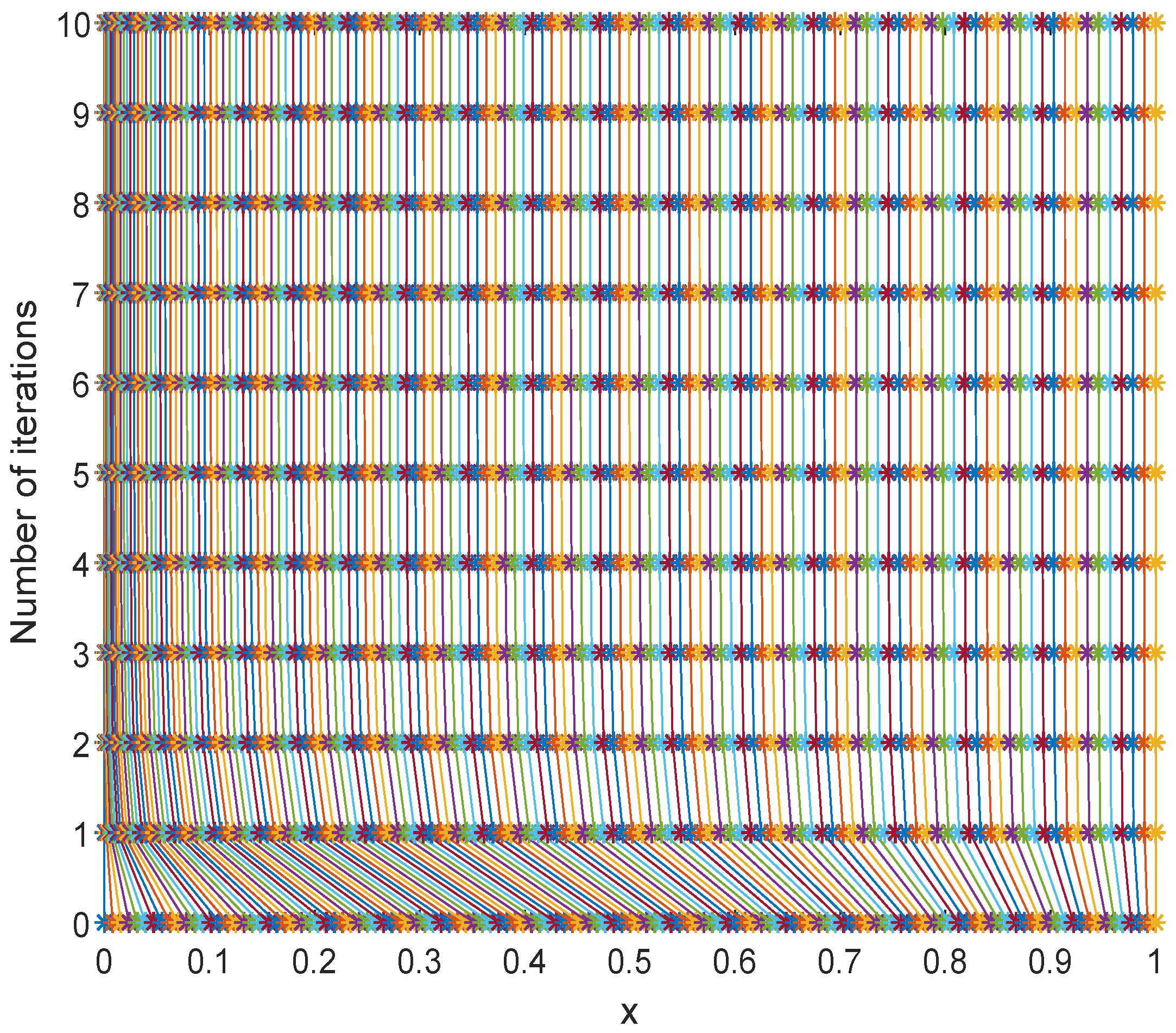
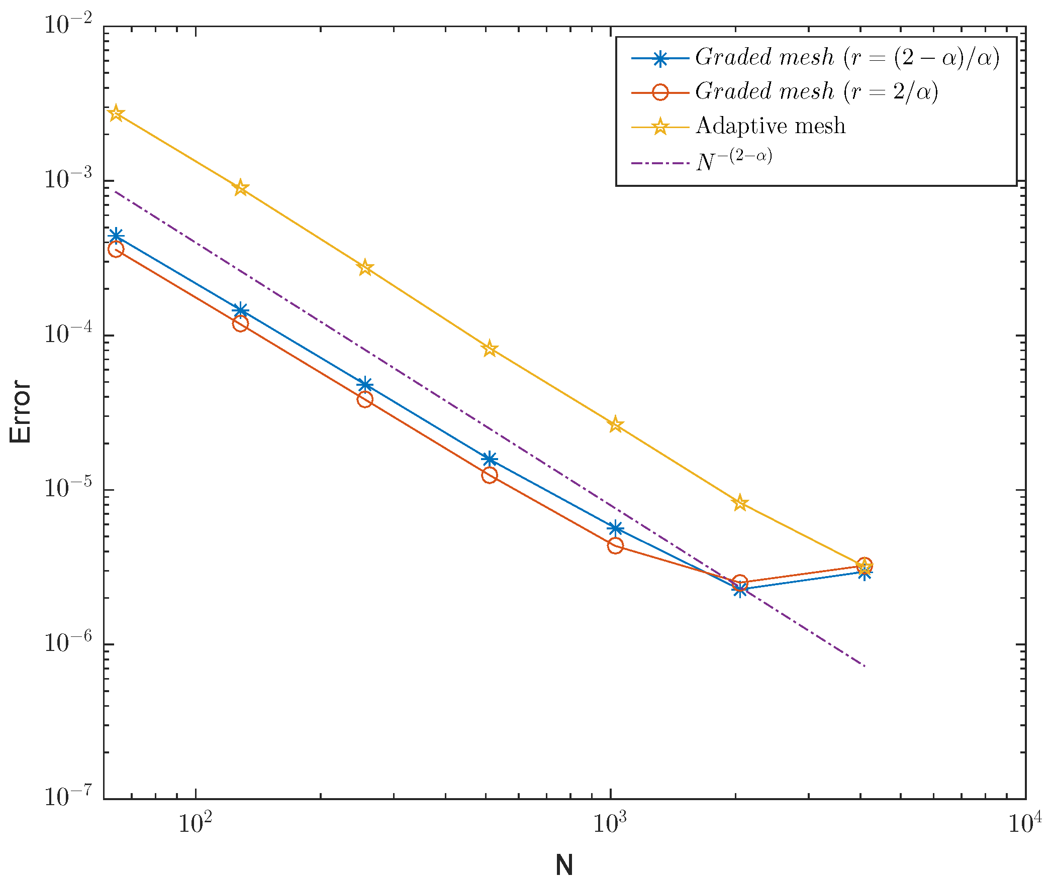
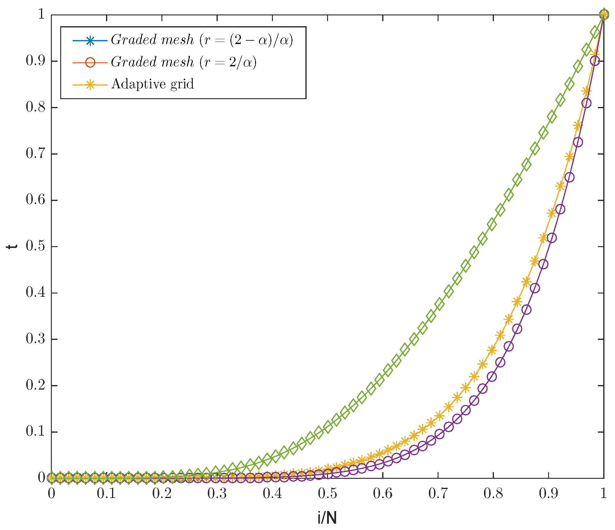
In addition, in order to verify the weak singularity of the solution of this test problem, Figure 1 displays the graphic of numerical solutions with N = 64 and different values of α . One can see from this figure that the solution of this test problem has a weakly singularity at t = 0 . When α = 0.8 , Figure 2 shows how a mesh with N = 128 intervals evolves through successive iterations of the algorithm. Obviously, with the increase in iteration times, more and more grid points move to t = 0 . In Figure 3, when α = 0.3 , the errors on the adaptive meshes are compared with the errors on the optimal graded mesh t j = T ( j / N ) r j = 0 N with r = ( 2 α ) / α and r = 2 / α . One can see from Figure 3 that the optimal rates of convergence 2 α of the presented adaptive grid are attained, but with increase of N, the rate of convergence of the graded mesh becomes smaller. This is because the graded meshes at the singularity attachment are more dense, see Figure 4.

6. Conclusions

This work mainly discussed a new adaptive grid approach for a nonlinear fractional differential equation with a Caputo derivative. Using Taylor expansion formula with integral remainder term, we derived a new truncation error estimation, which is utilized to construct an adaptive mesh generation algorithm. It is shown from the numerical experiments that the presented monitor function (34) can be successfully applied to a class of Caputo fractional initial value problems.
In addition, it should be pointed out that the proposed adaptive grid method in this paper can be extended to some time-fractional partial differential equations with Caputo fractional derivative, such as the time-fractional diffusion wave equations and the time fractional Allen–Cahn equation. Meanwhile, if we use a higher order accurate numerical scheme, such as L2 scheme, to approximate the Caputo fractional derivative, we can also design a second or even third order accurate adaptive gird method for problem (1).

Author Contributions

Conceptualization, T.Y.; Project administration, L.-B.L.; Writing—original draft, X.B.; Writing—review editing, Y.Z. All authors have read and agreed to the published version of the manuscript.

Funding

This work was supported by the Natural Science Foundation of Guangxi Province (2020GXNSFAA159010) and the projects of Excellent Young Talents Fund in Universities of Anhui Province (gxyq2021225).

Data Availability Statement

Not applicable.

Conflicts of Interest

The authors declare no conflict of interest.

References

  1. Stynes, M.; O’Riordan, E.; Gracia, J.L. Error analysis of a finite difference method on graded meshes for a time-fractional diffusion equation. SIAM J. Numer. Anal. 2017, 55, 1057–1079. [Google Scholar] [CrossRef] [Green Version]
  2. Magin, R. Fractional Calculus in Bioengineering; Begell House Publishers: Redding, CA, USA, 2006. [Google Scholar]
  3. Kaur, A.; Takhar, P.S.; Smith, D.M.; Mann, J.E.; Brashears, M.M. Fractional differential equations based modeling of microbial survival and growth curves: Model development and experimental validation. Food Eng. Phys. Prop. 2008, 73, E403–E414. [Google Scholar] [CrossRef]
  4. Lokenath, D. Recent applications of fractional calculus to science and engineering. Int. J. Math. Math. Sci. 2003, 54, 3413–3442. [Google Scholar]
  5. Jin, B.; Lazarov, R.; Pasciak, J.; Rundell, W. Variational formulation of problems involving fractional order differential operators. Math. Comput. 2015, 84, 2665–2700. [Google Scholar] [CrossRef] [Green Version]
  6. Diethelm, K. The Analysis of Fractional Differential Equations. An Application-Oriented Exposition Using Differential Operators of Caputo Type; Springer: Heidelberg, Germany, 2010. [Google Scholar]
  7. Kilbas, A.A.; Srivastava, H.M.; Trujillo, J.J. Theroy and Applications of Fractional Differential Equations; Elsevier: Amsterdam, The Netherlands, 2006. [Google Scholar]
  8. Machado, J.T.; Kiryakova, V.; Mainardi, F. Recent history of fractional calculus. Commun. Nonlinear Sci. Numer. Simul. 2011, 16, 1140–1153. [Google Scholar] [CrossRef] [Green Version]
  9. Chen, C.-M.; Liu, F.; Anh, V.; Turner, I. Numerical schemes with high spatial accuracy for a variable-order anomalous subdiffusion equation. SIAM J. Sci. Comput. 2010, 32, 1740–1760. [Google Scholar] [CrossRef]
  10. Gao, G.; Sun, Z. A compact finite difference scheme for the fractional sub-diffusion equations. J. Comput. Phys. 2011, 230, 586–595. [Google Scholar] [CrossRef]
  11. Liao, H.; Li, D.; Zhang, J. Sharp error estimate of the nonuniform L1 formula for linear reaction-subdiffusion equations. SIAM J. Numer. Anal. 2018, 56, 1112–1133. [Google Scholar] [CrossRef]
  12. Liao, H.; Mclean, W.; Zhang, J. A discrete Grönwall inequality with applications to numerical scheme for sudiffusion problems. SIAM J. Numer. Anal. 2019, 57, 218–237. [Google Scholar] [CrossRef]
  13. Gracia, J.L.; O’Riordan, E.; Stynes, M. A fitted scheme for a Caputo initial-boundary value problem. J. Sci. Comput. 2018, 76, 583–609. [Google Scholar] [CrossRef]
  14. Kopteva, N.; Meng, X. Error analysis for a fractional-derivative parabolic problem on quasi-graded meshes using barrier function. SIAM J. Numer. Anal. 2020, 58, 1217–1238. [Google Scholar] [CrossRef]
  15. Kopteva, N. Error analysis of the L1 method on graded and uniform meshes for a fractional-derivative problem in two and three dimensions. Math. Comput. 2019, 88, 2135–2155. [Google Scholar] [CrossRef]
  16. Jin, B.; Lazarov, R.; Zhou, Z. Numerical methods for time-fractional evolution equations with nonsmooth data: A concise overvies. Comput. Methods Appl. Mech. Eng. 2019, 346, 332–358. [Google Scholar] [CrossRef] [Green Version]
  17. Sun, Z.; Wu, X. A fully discrete difference scheme for a diffusion-wave system. Appl. Numer. Math. 2006, 56, 193–209. [Google Scholar] [CrossRef]
  18. Lin, Y.; Xu, C. Finite difference/spectral approximations for the time-fractional diffusion equation. J. Comput. Phys. 2007, 225, 1533–1552. [Google Scholar] [CrossRef]
  19. Liu, F.; Anh, V.; Turner, I. Numerical solution of the space fractional Fokker-Planck equation. J. Comput. Appl. Math. 2004, 166, 209–219. [Google Scholar] [CrossRef] [Green Version]
  20. Lynch, V.; Carreras, B.; del Castillo-Negrete, D.; Ferreira-Mejias, K.; Hicks, H. Numerical methods for the solution of partial differential equations of fractional order. J. Comput. Phys. 2003, 192, 406–421. [Google Scholar] [CrossRef]
  21. Du, R.; Cao, W.R.; Sun, Z.-Z. A compact difference scheme for the fractional diffusion-wave equation. Appl. Math. Model. 2010, 34, 2998–3007. [Google Scholar] [CrossRef]
  22. Du, R.; Yan, Y.; Liang, Z. A high-order scheme to approximate the Caputo fractional derivative and its application to solve the fractional diffusion wave equation. J. Comput. Phys. 2019, 376, 1312–1330. [Google Scholar] [CrossRef] [Green Version]
  23. Jin, B.; Lazarov, R.; Zhou, Z. An analysis of the L1 scheme for the subdiffusion equation with nonsmooth data. IMA J. Numer. Anal. 2016, 36, 197–221. [Google Scholar] [CrossRef] [Green Version]
  24. Jin, B.; Lazarov, R.; Zhou, Z. Two fully discrete schemes for fractional diffusion and diffusion-wave equations with nonsmooth data. SIAM J. Sci. Comput. 2016, 38, A146–A170. [Google Scholar] [CrossRef]
  25. Brunner, H. Collocation Methods for Volterra Integral and Related Functional Equations Methods; Cambridge University Press: Cambridge, UK, 2004. [Google Scholar]
  26. Cen, Z.; Le, A.; Xu, A. A posteriori error analysis for a fractional differential equation. Int. J. Comput. Math. 2017, 94, 1185–1195. [Google Scholar] [CrossRef]
  27. Liu, L.-B.; Chen, Y. A posteriori error estimation and adaptive strategy for a nonlinear fractional differential equation. Int. J. Comput. Math. 2022, 99, 240–246. [Google Scholar] [CrossRef]
  28. Kopteva, N. Pointwise-in-time a posteriori errror control for time-fractional parabolic equations. Appl. Math. Lett. 2022, 123, 107515. [Google Scholar] [CrossRef]
  29. Liu, L.-B.; Liang, Z.; Long, G.; Liang, Y. Convergence analysis of a finite difference scheme for a Riemann-Liouville fractional derivative two-point boundary value problem on an adaptive grid. J. Comput. Appl. Math. 2020, 375, 112809. [Google Scholar] [CrossRef]
  30. Cen, Z.; Liu, L.-B.; Huang, J. A posteriori error estimation in maximum norm for a two-point boundary value problem with a Riemann Liouville fractional derivative. Appl. Math. Lett. 2020, 102, 106086. [Google Scholar] [CrossRef]
  31. Huang, J.; Cen, Z.; Liu, L.B.; Zhao, J. An efficient numerical method for a Riemann-Liouville two-point boundary value problem. Appl. Math. Lett. 2020, 103, 106201. [Google Scholar] [CrossRef]
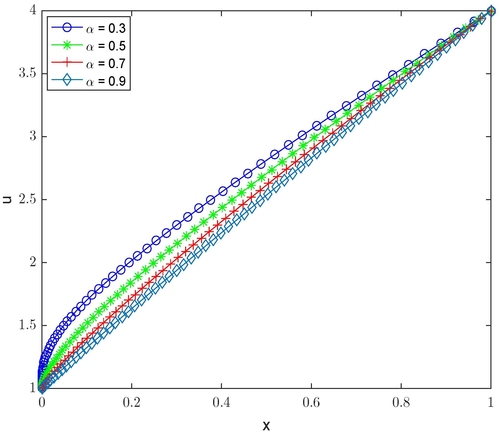
Figure 1. Numerical solutions with N = 64 and different values of α .
Fractalfract 06 00647 g001
Figure 2. Evolution of mesh with α = 0.8 and N = 128 .
Fractalfract 06 00647 g002
Figure 3. Convergence orders of adaptive grid and graded grids with α = 0.3 .
Fractalfract 06 00647 g003
Figure 4. The comparison of our adaptive mesh and graded meshes with α = 0.3 and N = 64 .
Fractalfract 06 00647 g004
Table 1. Numerical results using arc-length monitor function [26].
α N = 64 N = 128 N = 256 N = 512 N = 1024 N = 2048
0.3 E N 1.0172 × 10 2 6.9168 × 10 3 4.6847 × 10 3 3.6557 × 10 3 2.2172 × 10 3 2.3492 × 10 3
r N 0.55650.56220.35780.7213−0.0834
0.5 E N 1.0257 × 10 2 5.8439 × 10 3 3.2138 × 10 3 1.7763 × 10 3 1.0504 × 10 3 5.5770 × 10 4
r N 0.81160.86270.85540.75700.9134
0.7 E N 6.2524 × 10 3 3.5771 × 10 3 2.0053 × 10 3 1.0080 × 10 3 5.9720 × 10 4 3.2655 × 10 4
r N 0.80570.83500.85580.89170.8709
0.9 E N 2.1028 × 10 3 1.2125 × 10 3 6.8524 × 10 4 3.8084 × 10 4 2.0932 × 10 4 1.1346 × 10 4
r N 0.79430.82330.84740.86350.8836
Table 2. Errors and rates of convergence using our new monitor function (34).
α N = 64 N = 128 N = 256 N = 512 N = 1024 N = 2048
0.3 E N 2.6073 × 10 3 8.1996 × 10 4 2.3637 × 10 4 6.5119 × 10 5 1.7583 × 10 5 4.8644 × 10 6
r N 1.66891.79451.85991.88891.8539
0.5 E N 1.9314 × 10 3 5.6238 × 10 4 1.5345 × 10 4 5.1256 × 10 5 1.8145 × 10 5 6.4481 × 10 6
r N 1.78001.87381.58201.49821.4926
0.7 E N 1.6903 × 10 3 6.4963 × 10 4 2.5380 × 10 4 1.0091 × 10 4 4.0563 × 10 5 1.6397 × 10 5
r N 1.37961.35591.33061.31481.3066
0.9 E N 1.0563 × 10 3 4.9879 × 10 4 2.3273 × 10 4 1.0822 × 10 4 5.0327 × 10 5 2.3420 × 10 5
r N 1.08251.09971.10471.10461.1036
Publisher’s Note: MDPI stays neutral with regard to jurisdictional claims in published maps and institutional affiliations.