A Fractional Order Investigation of Smoking Model Using Caputo-Fabrizio Differential Operator

Abstract

Smoking is a social trend that is prevalent around the world, particularly in places of learning and at some significant events. The World Health Organization defines smoking as the most important preventable cause of disease and the third major cause of death in humans. In order to analyze this matter, this study typically emphasizes analyzing the dynamics of the fractional order quitting smoking model via the Caputo-Fabrizio differential operator. For the numerical solution of the considered model, the Laplace transform with the Adomian decomposition method (LADM) and Homotopy perturbation method (HPM) is applied, and the comparison of both the achieved numerical solutions is presented. Moreover, numerical simulation for the suggested scheme has been presented in various fractional orders with the aid of Matlab and the numerical results are supported by illustrative graphics. The simulation reveals the aptness of the considered model.

1. Introduction

Mathematical biology is a wide-ranging field with several applications. In this field, researchers are focusing on the portrayal of different types of diseases with controls in the form of mathematical models. In 1909, Brownlee [1] took the initiative for the growth of the field of mathematical biology and the emphasis was on the theory of fortuitous. Furthermore, in 1912, he presented the basic laws for epidemic spreading [2]. In 1927, Kermark and McKendrik [3] discussed the minutiae of the epidemic study. Later, many researchers discoursed different models of various other diseases; see [4,5,6,7]. On the other hand, one of the social habits that are spreading all over the world speedily as an infectious disease is smoking. Smoking is the process by which people inhale the smoke of tobacco containing particles and gas or simply [8,9]. Smoking is the practice in which smoke is taken into the mouth and then released utilizing pipes or cigars. Columbus was the first one who introduced smoking in Europe in the sixteenth-century [10], but before and after this date, many other exotic species were offered, with great contrary effects on ecosystems and effect on human habits [11,12]. Nicot spread tobacco as a cash crop in England; he was the first who used it as a business, and that is why the word nicotine derived from his name. Smoking can root different kinds of diseases together with mouth cancer, lung cancer, larynan, heart diseases, vascular diseases, respiratory diseases, and many other diseases that are injurious to human health [13,14,15].

Nowadays, smoking is one of the foremost health problems in the world. According to the world health organization (WHO) report on the smoking, epidemic [16], smoking kills numerous people in their most active life. More than 5 million deaths in the world are caused due to the effect of smoking on different organs of the human body, which may increase to up to 8 million people per year by 2030 [17,18]. The chance of heart attack is $70\%$ more in smokers equated to the persons who are not smoking. Smokers have a $10\%$ higher incidence rate of lung cancer than that nonsmokers. The life of smokers is 10 to 13 years shorter than that of non-smokers. Mathematician tries to control smoking for securing the life expectancy of an individual. To give the best illustration of cigarette smoking phenomena, mathematicians tried to make different effective smoking models. The different smoking models were proposed by several authors. For the first time in the year of 1997, Castillo-Garsow [19] outlined a mathematical model for smoking and divide the total population into three different classes (potential smokers, chain smokers and permanently quit smokers). In 2007, Ham [20] documented the different stages and procedures of smoking among students through a survey in different vocational-technical schools in Korea. In 2008, Sharomi and Gumel [14] improved their model to present a new temporarily quit smokers class. Zaman [21] extended the model by presenting a new occasional smokers class and offered a dynamical interaction in an integer order. Several others presented the smoking models in integer and fractional order. Erturk [22] studied a giving up smoking model associated with the Caputo fractional derivative. Zeb [23] examined a fractional giving up smoking. Alkhudhari [24] analyzed the global dynamics of mathematical equations describing smoking. Khalid [25] described the fractional mathematical model of giving up smoking and many others.

We can utilize mathematical modeling to prevent the spread of tobacco smoking because it has been used as a significant tool for pandemic grasp in recent decades. The susceptible-exposed-infected-recovered (SEIR) is a general model. Therefore, the model under consideration for this study is described as follows:

$$\left\{\begin{array}{cc}& {\displaystyle \frac{dX\left(t\right)}{d\left(t\right)}}=\lambda -{\beta }_{1}X\left(t\right)H\left(t\right)+\alpha Y\left(t\right)-\mu X\left(t\right),\hfill \\ \hfill & {\displaystyle \frac{dH\left(t\right)}{dt}}={\beta }_{1}X\left(t\right)H\left(t\right)-{\beta }_{2}H\left(t\right)J\left(t\right)-({\lambda }_1+\mu )H\left(t\right),\hfill \\ & {\displaystyle \frac{dJ\left(t\right)}{dt}}={\beta }_{2}H\left(t\right)J\left(t\right)-(\omega +{\lambda }_2+\mu )J\left(t\right)),\hfill \\ & {\displaystyle \frac{dY\left(t\right)}{dt}}=\omega J\left(t\right)-(\gamma +\mu +\alpha )Y\left(t\right),\hfill \\ & {\displaystyle \frac{dZ\left(t\right)}{dt}}=\gamma Y\left(t\right)-\mu Z\left(t\right).\hfill \end{array}\right.$$

(1)

We divided the total population into five classes, where $X\left(t\right)$ is susceptible smokers, $H\left(t\right)$ is the snuffing (ingestion) class, $J\left(t\right)$ is irregular smokers, $Y\left(t\right)$ is regular smokers, and $Z\left(t\right)$ is quit smokers, respectively, at a time t. The whole description of the parameters used in the model (1) is given in the

Table 1. Description of the model parameters.

Notation	Description of the Parameters
$\lambda$	The frequency of recruitment (birth or migration)
${\beta }_1$	The rate of the vulnerable population transitions to the snuffing class
${\beta }_2$	The Rate of snuffing becomes an irregular smokers
$\omega$	Rate of irregular smokers turning to a regular smoker
$\gamma$	Departing rate
$\mu$	Rate of natural death
$\alpha$	Rate of recovery
${\lambda }_1$	Rate of snuffing class deaths because of smoking
${\lambda }_2$	Rate of death due to smoking

mbelow:

In the last few decades, several biological models were studied in detail with the thought of classical derivatives, including [26,27,28,29,30,31,32,33]. Since in recent years fractional calculus has fascinated great attention from researchers and various features of the said subject are under consideration for research. This is because of the reality that fractional derivative is an important tool to explain the dynamical behavior of various physical systems [34,35]. The specialty of these differential operators is their non-local physiognomies which do not exist in the integer order differential operators [36,37]. As a fact, fractional order models are more accurate and practical than the classical integer order models [38,39,40]. Fractional order derivative produces a better degree of freedom in these models. Arbitrary order derivatives are powerful tools for the discretion of the dynamical behavior of various bio-materials and systems [41,42,43]. This is why there are different fractional derivatives; Riemann and Liouville, and Caputo operators are the most conservative examples in traditional practice. Caputo [44] presented a fractional derivative that permits the conventional initial and boundary conditions allied with the real-world problem. Although the aforesaid derivatives show more accuracy in describing real phenomena compared to the integer-order derivatives, their kernel functions yield singularities which result in a multitude of computational deficiencies. Moreover, to examine fractional mathematical models outside of the traditional Caputo derivative notion, several methodologies, such as iterative and numerical methods, have been applied [45].

In a recent effort, a new derivative that is non-singular and comprises an exponential law kernel has latterly been brought into operation by Caputo and Fabrizio [46], and aptly titled after them as Caputo-Fabrizio (CF) derivative. Losada and Nieto [47] presented the fractional integral corresponding to the newly offered fractional derivative and analyzed some related fractional differential equations. The classical fractional derivatives, specifically the Caputo and Riemann derivatives, have their constraint as their kernel is singular which causes complications in fractional order derivatives. Since the kernel is employed to define the memory effect of the physical system, it is obvious that as a result of this weakness, both derivatives cannot exactly describe the full effect of the memory. Generally, it is not simple for non-linear fractional differential equations to obtain their general solutions. Therefore, the new type of non-singular derivatives of fractional order has been found more suitable for studying thermal problems instead of ordinary derivatives. Moreover, it is evident from the research which has been carried out pursuant to these advancements in recent years that these fractional derivatives provide scientists a good chance to describe diverse problems. To overwhelm this condition, various methods are outlined in the existing literature to determine the approximate solutions for the nonlinear systems [48]. Runge Kutta methods were widely employed in handling mathematical analysis [49]. The Homotopy perturbation method (HPM), Laplace Adomian decomposition method (LADM), and method of difference have been widely used to deal with both linear and non-linear fractional order differential equations [50,51,52,53,54]. Therefore, inspired by the applicability of these non-singular derivatives, we aim to further analyze the smoking model in view of the fractional concept and to explicate this problem in a better and more effective manner.

In the present study, to obtain a better understanding of the qualitative analysis as well as the numerical iterative analysis of the proposed model, the revised form of the model (1) in the sense of Caputo-Fabrizio fractional derivative (CFFD) is considered which is described as follows:

$$\left\{\begin{array}{cc}{}^{CF}{D}_t^p\left(X\right)\left(t\right)=\lambda -{\beta }_{1}X\left(t\right)H\left(t\right)+\alpha Y\left(t\right)-\mu X\left(t\right),\hfill & \\ {}^{CF}{D}_t^p\left(H\right)\left(t\right)={\beta }_{1}X\left(t\right)H\left(t\right)-{\beta }_{2}H\left(t\right)J\left(t\right)-({\lambda }_1+\mu )H\left(t\right),\hfill & \\ {}^{CF}{D}_t^{p}J\left(t\right)={\beta }_{2}H\left(t\right)J\left(t\right)-(\omega +{\lambda }_2+\mu )J\left(t\right),\hfill & \\ {}^{CF}{D}_t^p\left(Y\right)\left(t\right)=\omega J\left(t\right)-(\gamma +\mu +\alpha )Y\left(t\right),\hfill & \\ {}^{CF}{D}_t^p\left(Z\right)\left(t\right)=\gamma Y\left(t\right)-\mu Z\left(t\right),\hfill \end{array}\right.$$

(2)

subject to the initial conditions:

$$X\left(0\right)=m_1,H\left(0\right)=m_2,J\left(0\right)=m_3,Y\left(0\right)=m_4,Z\left(0\right)=m_5.$$

The goal of this work is to investigate the dynamical behavior of the smoking mathematical model with the help of the Caputo-Fabrizio differential operator and makes use of the utilities of fractional calculus. The Laplace transform with the Adomian decomposition method and the Homotopy perturbation method are employed to achieve the approximate solution of the considered model. As well as the comparison of the obtained results of both techniques is presented which shows the identical character. Moreover, the numerical solutions are facilitated with the aid of MATLAB and the graphical representation of each compartment is shown in arbitrary fractional order.

The distribution of this paper is ordered as follows: We start with some fundamental results and definitions in Section 2. In Section 3, the analytical solution of the suggested model utilizing the Laplace Adomian decomposition approach and the Homotopy perturbation method is estimated. The numerical simulations to validate and backing the analytical findings of the aforementioned sections are performed. In Section 4, the comparison of both numerical solutions achieved from the aforementioned schemes is shown graphically and the obtained numerical simulation results are briefly discussed. Finally, the concluding remarks of this study are given in Section 5.

2. Analytical Preliminaries

This section is devoted to certain essential terminologies and fractional calculus results in line with [55,56].

Definition 1.

Let $f\in$$H^1[0,\alpha ]$, $\alpha >0$, $p\in (0,1)$, then the Caputo-Fabrizio fractional derivative of the function $f\left(t\right)$ is described as follows:

$${}^{CF}{D}_t^p\left[f\left(t\right)\right]={\displaystyle \frac{M\left(p\right)}{1-p}}{\int }_0^t{f}^{\prime }\left(x\right)exp[-p{\displaystyle \frac{t-x}{1-p}}]dx,$$

where $M\left(p\right)$ represents the normalization function and $M\left(0\right)=M\left(1\right)=1$.

Definition 2.

The Caputo-Fabrizio fractional integral with $p\in (0,1)$ for a function f is describes as follows:

$${}^{CF}{I}_t^p\left[f\left(t\right)\right]={\displaystyle \frac{1-p}{N\left(p\right)}}+{\displaystyle \frac{p}{N\left(p\right)}}{\int }_0^{t}f\left(x\right)dx,t\ge 0.$$

Definition 3.

The general formula for the Laplace Transform of Caputo-Fabrizio fractional derivative is described as follows:

$$\begin{array}{c}\hfill 𝓛{[}^{CF}{D}_t^p\left[f\left(t\right)\right]={\displaystyle \frac{s\mathcal{𝓛}\left[f\right(t\left)\right]-f\left(0\right)}{s+p(1-s)}},s\ge 0.\end{array}$$

Definition 4.

The homotopy perturbation method (HPM) is a semi-analytical technique for the solution of linear and nonlinear ordinary as well as partial differential equations and systems. A system of paired linear and nonlinear differential equations may also be estimated via this approach. One clear advantage of using the HPM compared to decomposition would be that it can handle nonlinear problems without the requirement for Adomian’s polynomial. Moreover, “He” was the Chinese mathematician who first proposed the idea of HPM. The authors in [57] applied the HPM to nonlinear oscillator problem. It could be used in an equation having linear and nonlinear parts, and one can form a homotopy $\nu (s,p):D\times [0,1]\to R:$

$$F(\nu ,p)=(1-p)[L\left(\nu \right)-L\left(u_0\right)]+p[L\left(\nu \right)+N\left(\nu \right)-f\left(s\right)]=0,$$

(3)

where L is used for the linear part, N for the nonlinear part, $s\in D$, D is a topological space and $p\in [0,1]$ is the embedding parameter. Further, $u_0$ is an initial approximation that satisfies the boundary conditions.

Definition 5.

([58]). The He’s fractional derivative is defined as:

$$\begin{array}{c}\hfill D_t^p=\frac{1}{\Gamma (n-p)}\frac{d^n}{d{t}^n}{\int }_{t_0}^t{(s-t)}^{n-p-1}[f_0\left(s\right)-f\left(s\right)]ds.\end{array}$$

(4)

3. General Solution for the Model (2)

In this section, we discuss the general techniques to construct the solution for the considered model (2) along with the initial conditions.

3.1. General Solution for Model (2) with (LADM)

Now, taking the Laplace transform of the considered (2), and the normalization value $M\left(p\right)=1$, one may get

$$\left\{\begin{array}{cc}\mathcal{𝓛}{[}^{CF}{D}_t^p\left(X\right)\left(t\right)]=\mathcal{𝓛}[\lambda -{\beta }_{1}X\left(t\right)H\left(t\right)+\alpha Y\left(t\right)-\mu X\left(t\right)],\hfill & \\ \mathcal{𝓛}{[}^{CF}{D}_t^p\left(H\right)\left(t\right)]=\mathcal{𝓛}[{\beta }_{1}X\left(t\right)H\left(t\right)-{\beta }_{2}H\left(t\right)J\left(t\right)-({\lambda }_1+\mu )H\left(t\right)],\hfill & \\ \mathcal{𝓛}{[}^{CF}{D}_t^p\left(J\right)\left(t\right)]=\mathcal{𝓛}[{\beta }_{2}H\left(t\right)J\left(t\right)-(\omega +{\lambda }_2+\mu )J\left(t\right)],\hfill & \\ \mathcal{𝓛}{[}^{CF}{D}_t^p\left(Y\right)\left(t\right)]=\mathcal{𝓛}[\omega J\left(t\right)-(\gamma +\mu +\alpha )Y\left(t\right)],\hfill & \\ \mathcal{𝓛}{[}^{CF}{D}_t^p\left(Z\right)\left(t\right)]=\mathcal{𝓛}[\gamma Y\left(t\right)-\mu Z\left(t\right)].\hfill \end{array}\right.$$

(5)

Using the initial conditions yields

$$\left\{\begin{array}{cc}\mathcal{𝓛}\left[\left(X\right)\left(t\right)\right]={\displaystyle \frac{X\left(0\right)}{s}}+{\displaystyle \frac{s+p(1-s)}{s}}\mathcal{𝓛}[\lambda -{\beta }_{1}X\left(t\right)H\left(t\right)+\alpha Y\left(t\right)-\mu X\left(t\right)],\hfill & \\ \mathcal{𝓛}\left[\left(H\right)\left(t\right)\right]={\displaystyle \frac{H\left(0\right)}{s}}+{\displaystyle \frac{s+p(1-s)}{s}}\mathcal{𝓛}[{\beta }_{1}X\left(t\right)H\left(t\right)-{\beta }_{2}H\left(t\right)J\left(t\right)-({\lambda }_1+\mu )H\left(t\right)],\hfill & \\ \mathcal{𝓛}\left[\left(J\right)\left(t\right)\right]={\displaystyle \frac{J\left(0\right)}{s}}+{\displaystyle \frac{s+p(1-s)}{s}}\mathcal{𝓛}[{\beta }_{2}H\left(t\right)J\left(t\right)-(\omega +{\lambda }_2+\mu )J\left(t\right)],\hfill & \\ \mathcal{𝓛}\left[\left(Y\right)\left(t\right)\right]={\displaystyle \frac{Y\left(0\right)}{s}}-{\displaystyle \frac{s+p(1-s)}{s}}\mathcal{𝓛}[\omega J\left(t\right)-(\gamma +\mu +\alpha )Y\left(t\right)],\hfill & \\ \mathcal{𝓛}\left[\left(Z\right)\left(t\right)\right]={\displaystyle \frac{Z\left(0\right)}{s}}-{\displaystyle \frac{s+p(1-s)}{s}}\mathcal{𝓛}[\gamma Y\left(t\right)-\mu Z\left(t\right)].\hfill \end{array}\right.$$

(6)

Assuming the solution for the compartments $X\left(t\right),H\left(t\right),J\left(t\right),Y\left(t\right)$, and $Z\left(t\right)$ in an infinite series is given below:

$$\begin{array}{c}\left\{\begin{array}{c}X\left(t\right)=\sum _{k=0}^{\infty }{X}_k\left(t\right),H\left(t\right)=\sum _{k=0}^{\infty }{H}_k\left(t\right),\hfill \\ J_k\left(t\right)=\sum _{k=0}^{\infty }{J}_k\left(t\right),Y\left(t\right)=\sum _{k=0}^{\infty }{Y}_k\left(t\right),\hfill \\ Z\left(t\right)=\sum _{k=0}^{\infty }{Z}_k\left(t\right),\hfill \end{array}\right.\end{array}$$

(7)

where $X\left(t\right)H\left(t\right)={\sum }_{k=0}^{\infty }{S}_k\left(t\right)$, $H\left(t\right)J\left(t\right)={\sum }_{k=0}^{\infty }W\left(t\right)$ are the non-linear terms of Adomian polynomial wherein:

$$\left\{\begin{array}{c}{S}_k\left(t\right)=\frac{1}{m!}\frac{d^m}{d{\lambda }^m}\left[\sum _{k=0}^m{\lambda }^k{X}_k\left(t\right)\sum _{k=0}^m{\lambda }^k{H}_k\left(t\right)\right]{|}_{\lambda =0},\hfill \\ W_k\left(t\right)=\frac{1}{m!}\frac{d^m}{d{\lambda }^m}\left[\sum _{k=0}^m{\lambda }^k{H}_k\left(t\right)\sum _{k=0}^m{\lambda }^k{J}_k\left(t\right)\right]{|}_{\lambda =0}.\hfill \end{array}\right.$$

(8)

Using Equations (7) and (8) into (6), one can get

$$\left\{\begin{array}{cc}\mathcal{𝓛}\left[\sum _{k=0}^{\infty }{X}_k\left(t\right)\right]={\displaystyle \frac{X\left(0\right)}{s}}+{\displaystyle \frac{s+p(1-s)}{s}}\mathcal{𝓛}[\lambda -{\beta }_1\sum _{k=0}^{\infty }{S}_k\left(t\right)+\alpha \sum _{k=0}^{\infty }{Y}_k\left(t\right)-\mu \sum _{k=0}^{\infty }{X}_k\left(t\right)],\hfill & \\ \mathcal{𝓛}\left[\sum _{k=0}^{\infty }{H}_k\left(t\right)\right]={\displaystyle \frac{H\left(0\right)}{s}}+{\displaystyle \frac{s+p(1-s)}{s}}\mathcal{𝓛}[{\beta }_1\sum _{k=0}^{\infty }{S}_k\left(t\right)-{\beta }_2\sum _{k=0}^{\infty }W\left(t\right)-({\lambda }_1+\mu )\sum _{k=0}^{\infty }{H}_k\left(t\right)],\hfill & \\ \mathcal{𝓛}\left[\sum _{k=0}^{\infty }{J}_k\left(t\right)\right]={\displaystyle \frac{J\left(0\right)}{s}}+{\displaystyle \frac{s+p(1-s)}{s}}\mathcal{𝓛}[{\beta }_2\sum _{k=0}^{\infty }W\left(t\right)-(\omega +{\lambda }_2+\mu )\sum _{k=0}^{\infty }{J}_k\left(t\right)],\hfill & \\ \mathcal{𝓛}\left[\sum _{k=0}^{\infty }{Y}_k\left(t\right)\right]={\displaystyle \frac{Y\left(0\right)}{s}}+{\displaystyle \frac{s+p(1-s)}{s}}\mathcal{𝓛}[\omega \sum _{k=0}^{\infty }{J}_k\left(t\right)-(\gamma +\mu +\alpha )\sum _{k=0}^{\infty }{Y}_k\left(t\right)],\hfill & \\ \mathcal{𝓛}\left[\sum _{k=0}^{\infty }{Z}_k\left(t\right)\right]={\displaystyle \frac{Z\left(0\right)}{s}}+{\displaystyle \frac{s+p(1-s)}{s}}\mathcal{𝓛}[\gamma \sum _{k=0}^{\infty }{Y}_k\left(t\right)-\mu \sum _{k=0}^{\infty }{Z}_k\left(t\right)].\hfill \end{array}\right.$$

(9)

Now, comparing like terms on both sides, one can get

$$\left\{\begin{array}{c}\mathcal{𝓛}\left[X_0\left(t\right)\right]=\frac{m_1}{s},\mathcal{𝓛}\left[H_0\left(t\right)\right]=\frac{m_2}{s},\mathcal{𝓛}\left[J_0\left(t\right)\right]=\frac{m_3}{s},\mathcal{𝓛}\left[Y_0\left(t\right)\right]=\frac{m_4}{s},\mathcal{𝓛}\left[Z_0\left(t\right)\right]=\frac{m_5}{s},\hfill \\ \mathcal{𝓛}\left[X_1\left(t\right)\right]={\displaystyle \frac{s+p(1-s)}{s}}\mathcal{𝓛}[\lambda -{\beta }_1{S}_0\left(t\right)+\alpha Y_0\left(t\right)-\mu X_0\left(t\right)],\hfill & \\ \mathcal{𝓛}\left[H_1\left(t\right)\right]={\displaystyle \frac{s+p(1-s)}{s}}\mathcal{𝓛}[{\beta }_1{S}_0\left(t\right)-{\beta }_2{W}_0\left(t\right)-({\lambda }_1+\mu )H_0\left(t\right)],\hfill & \\ \mathcal{𝓛}\left[J_1\left(t\right)\right]=[{\beta }_2{W}_0\left(t\right)-(\omega +{\lambda }_2+\mu )J_0\left(t\right)],\hfill & \\ \mathcal{𝓛}\left[Y_1\left(t\right)\right]={\displaystyle \frac{s+p(1-s)}{s}}\mathcal{𝓛}[\omega J_0\left(t\right)-(\gamma +\mu +\alpha )Y_0\left(t\right)],\hfill & \\ \mathcal{𝓛}\left[Z_1\left(t\right)\right]={\displaystyle \frac{s+p(1-s)}{s}}\mathcal{𝓛}[\gamma Y_0\left(t\right)-\mu Z_0\left(t\right)],\hfill & \\ \mathcal{𝓛}\left[X_2\left(t\right)\right]={\displaystyle \frac{s+p(1-s)}{s}}\mathcal{𝓛}[\lambda -{\beta }_1{S}_1\left(t\right)+\alpha Y_1\left(t\right)-\mu X_1\left(t\right)],\hfill & \\ \mathcal{𝓛}\left[H_2\left(t\right)\right]={\displaystyle \frac{s+p(1-s)}{s}}\mathcal{𝓛}[{\beta }_1{S}_1\left(t\right)-{\beta }_2{W}_1\left(t\right)-({\lambda }_1+\mu )H_1\left(t\right)],\hfill & \\ \mathcal{𝓛}\left[J_2\left(t\right)\right]=[{\beta }_2{W}_1\left(t\right)-(\omega +{\lambda }_2+\mu )J_1\left(t\right)],\hfill & \\ \mathcal{𝓛}\left[Y_2\left(t\right)\right]={\displaystyle \frac{s+p(1-s)}{s}}\mathcal{𝓛}[\omega J_1\left(t\right)-(\gamma +\mu +\alpha )Y_1\left(t\right)],\hfill & \\ \mathcal{𝓛}\left[Z_2\left(t\right)\right]={\displaystyle \frac{s+p(1-s)}{s}}\mathcal{𝓛}[\gamma Y_1\left(t\right)-\mu Z_1\left(t\right)],\hfill \\ ⋮\hfill \\ \mathcal{𝓛}\left[X_{k+1}\left(t\right)\right]={\displaystyle \frac{s+p(1-s)}{s}}\mathcal{𝓛}[\lambda -{\beta }_1{S}_k\left(t\right)+\alpha Y_k\left(t\right)-\mu X_k\left(t\right)],\hfill & \\ \mathcal{𝓛}\left[H_{k+1}\left(t\right)\right]={\displaystyle \frac{s+p(1-s)}{s}}\mathcal{𝓛}[{\beta }_1{S}_k\left(t\right)-{\beta }_2{W}_k\left(t\right)-({\lambda }_1+\mu )H_k\left(t\right)],\hfill & \\ \mathcal{𝓛}\left[J_{k+1}\left(t\right)\right]=[{\beta }_2{W}_k\left(t\right)-(\omega +{\lambda }_2+\mu )J_k\left(t\right)],\hfill & \\ \mathcal{𝓛}\left[Y_{k+1}\left(t\right)\right]={\displaystyle \frac{s+p(1-s)}{s}}\mathcal{𝓛}[\omega J_k\left(t\right)-(\gamma +\mu +\alpha )Y_k\left(t\right)],\hfill & \\ \mathcal{𝓛}\left[Z_{k+1}\left(t\right)\right]={\displaystyle \frac{s+p(1-s)}{s}}\mathcal{𝓛}[\gamma Y_k\left(t\right)-\mu Z_k\left(t\right)].\hfill \end{array}\right.$$

(10)

Further, utilizing the inverse Laplace transform to equation (10), we have

$$\left\{\begin{array}{cc}{X}_0=m_1,H_0=m_2,J_0=m_3,Y_0=m_4,Z_0=m_5.\hfill & \\ X_1\left(t\right)=[\lambda -{\beta }_1{m}_1{m}_2+\alpha m_4-\mu m_1][1+p(t-1)],\hfill & \\ H_1\left(t\right)=[{\beta }_1{m}_1{m}_2-{\beta }_2{m}_2{m}_3-({\lambda }_1+\mu )m_2][1+p(t-1)],\hfill & \\ J_1\left(t\right)=[{\beta }_2{m}_2{m}_3-(\omega +{\lambda }_2+\mu )m_3][1+p(t-1)],\hfill & \\ Y_1\left(t\right)=[\omega m_3-(\gamma +\mu +\alpha )m_4][1+p(t-1)],\hfill & \\ Z_1\left(t\right)=[\gamma m_4-\mu m_5][1+p(t-1)].\hfill & \\ X_2\left(t\right)=[\lambda ][1+p(t-1)]+[-{\beta }_1(x_{11}{m}_2+m_1{h}_{11})+(\alpha y_{11}-\mu x_{11})][p^2{t}^2-2p^{2}t+2pt+{(p-1)}^2],\hfill & \\ H_2\left(t\right)=[{\beta }_1(x_{11}{m}_2+m_1{h}_{11})-{\beta }_2(m_2{J}_{11}+m_3{h}_{11})+({\lambda }_1+\mu )h_{11}][p^2{t}^2-2p^{2}t+2pt+{(p-1)}^2],\hfill & \\ J_2\left(t\right)=[{\beta }_2(m_2{J}_{11}+m_3{h}_{11})-(\omega +{\lambda }_2+\mu )J_{11}][p^2{t}^2-2p^{2}t+2pt+{(p-1)}^2],\hfill & \\ Y_2\left(t\right)=[\omega J_{11}-(\gamma +\mu +\alpha )y_{11}][p^2{t}^2-2p^{2}t+2pt+{(p-1)}^2],\hfill & \\ Z_2\left(t\right)=[\gamma y_{11}-\mu z_{11}][p^2{t}^2-2p^{2}t+2pt+{(p-1)}^2].\hfill \end{array}\right.$$

(11)

Furthermore, the other terms can be obtained similarly, respectively, and the unknown values in the aforementioned equations are given underneath as:

$$\left\{\begin{array}{cc}{x}_{11}\left(t\right)=[\lambda -{\beta }_1{m}_1{m}_2+\alpha m_4-\mu m_1][1+p(t-1)],\hfill & \\ h_{11}\left(t\right)=[{\beta }_1{m}_1{m}_2-{\beta }_2{m}_2{m}_3-({\lambda }_1+\mu )m_2][1+p(t-1)],\hfill & \\ j_{11}\left(t\right)=[{\beta }_2{m}_2{m}_3-(\omega +{\lambda }_2+\mu )m_3][1+p(t-1)],\hfill & \\ y_{11}\left(t\right)=[\omega m_3-(\gamma +\mu +\alpha )m_4][1+p(t-1)],\hfill & \\ z_{11}\left(t\right)=[\gamma m_4-\mu m_5][1+p(t-1)].\hfill \end{array}\right.$$

(12)

3.2. Numerical Results and Simulations

In this section, we accomplish the numerical simulations to help the analytical findings of our proposed model. Therefore, we apportioned some values for the parameters which are used in the proposed model (2) as:

$$\left\{\begin{array}{c}{m}_1=68,m_2=40,m_3=30,m_4=20,m_5=15,\hfill \\ \lambda =0.1,{\beta }_1=0.003,{\beta }_2=0.002,\omega =0.05,\hfill \\ \gamma =0.05,\mu =0.002,\alpha =0.003,{\lambda }_1=0.003,{\lambda }_2=0.003.\hfill \end{array}\right.$$

Utilizing these parametric values, the following terms of the model (2) are obtained:

$$\left\{\begin{array}{cc}{X}_0=68,H_0=40,J_0=30,Y_0=20,Z_0=15.\hfill & \\ X_1=(-8.13)[1+p(t-1)],H_1=\left(5.58\right)[1+p(t-1)],J_1=\left(2.13\right)[1+p(t-1)],\hfill & \\ Y_1=(-0.98)[1+(y-1)],Z_1=\left(0.97\right)[1+p(t-1)],\hfill & \\ X_2=\left(0.1\right)[1+p(t-1)]-\left(0.1819\right)[p^2{t}^2-2p^{2}t+2pt+{(p-1)}^2],\hfill & \\ H_2=\left(0.2267\right)[p^2{t}^2-2p^{2}t+2pt+{(p-1)}^2],\hfill & \\ J_2=\left(0.486\right)[p^2{t}^2-2p^{2}t+2pt+{(p-1)}^2],\hfill & \\ Y_2=\left(0.0624\right)[p^2{t}^2-2p^{2}t+2pt+{(p-1)}^2],\hfill & \\ Z_2=(-0.0509)[p^2{t}^2-2p^{2}t+2pt+{(p-1)}^2].\hfill \end{array}\right.$$

(13)

Furthermore, the solutions to the first few terms are given as:

$$\left\{\begin{array}{cc}X\left(t\right)=68-\left(8.03\right)[1+p(t-1)]-\left(0.1819\right)[p^2{t}^2-2p^{2}t+2pt+{(p-1)}^2],\hfill & \\ H\left(t\right)=40+\left(5.58\right)[1+p(t-1)]+\left(0.2267\right)[p^2{t}^2-2p^{2}t+2pt+{(p-1)}^2],\hfill & \\ J\left(t\right)=30+(2,13)[1+p(t-1)]+\left(0.486\right)[p^2{t}^2-2p^{2}t+2pt+{(p-1)}^2],\hfill & \\ Y\left(t\right)=20-(-0.98)[1+(y-1)]+\left(0.0624\right)[p^2{t}^2-2p^{2}t+2pt+{(p-1)}^2],\hfill & \\ Z\left(t\right)=15+\left(0.97\right)[1+p(t-1)]-(-0.0509)[p^2{t}^2-2p^{2}t+2pt+{(p-1)}^2].\hfill \end{array}\right.$$

(14)

Note that from (14), one can obtain the approximate solution of the proposed model for various values of p.

3.3. General Solution for Model (2) with (HPM)

Now, we will employ the Homotopy perturbation method (HPM) to construct the general solution of the Model (2) as:

$$\left\{\begin{array}{cc}(1-q){[}^{CF}{D}_t^p\left(X\right)\left(t\right){-}^{CF}{D}_t^p\left(X_0\right)\left(t\right)]+q{[}^{CF}{D}_t^p\left(X\right)\left(t\right)-\lambda +{\beta }_{1}X\left(t\right)H\left(t\right)-\alpha Y\left(t\right)+\mu X\left(t\right)]=0,\hfill & \\ (1-q){[}^{CF}{D}_t^p\left(H\right)\left(t\right){-}^{CF}{D}_t^p{\left(H\right)}_0\left(t\right)]+q{[}^{CF}{D}_t^p\left(H\right)\left(t\right)-{\beta }_{1}X\left(t\right)H\left(t\right)+{\beta }_{2}H\left(t\right)J\left(t\right)+({\lambda }_1-\mu )H\left(t\right)]=0,\hfill & \\ (1-q){[}^{CF}{D}_t^p\left(J\right)\left(t\right){-}^{CF}{D}_t^p{\left(J\right)}_0\left(t\right)]+q{[}^{CF}{D}_t^p\left(J\right)\left(t\right)-{\beta }_{2}H\left(t\right)J\left(t\right)+(\omega +{\lambda }_2-\mu )J\left(t\right)]=0,\hfill & \\ (1-q){[}^{CF}{D}_t^p\left(Y\right)\left(t\right){-}^{CF}{D}_t^p\left(Y_0\right)\left(t\right)]+{[}^{CF}{D}_t^p\left(Y\right)\left(t\right)-\omega J\left(t\right)+(\gamma +\mu +\alpha )Y\left(t\right)]=0,\hfill & \\ (1-q){[}^{CF}{D}_t^p\left(Z\right)\left(t\right){-}^{CF}{D}_t^p\left(Z_0\right)\left(t\right)]+q{[}^{CF}{D}_t^p\left(Z\right)\left(t\right)-\gamma Y\left(t\right)+\mu Z\left(t\right)]=0.\hfill \end{array}\right.$$

(15)

Substituting $q=0$ in (15) yields the following system of fractional differential equations:

$$\left\{\begin{array}{cc}{}^{CF}{D}_t^p\left(X\right)\left(t\right){-}^{CF}{D}_t^p\left(X_0\right)\left(t\right)=0,\hfill & \\ {}^{CF}{D}_t^p\left(H\right)\left(t\right){-}^{CF}{D}_t^p{\left(H\right)}_0\left(t\right)=0,\hfill & \\ {}^{CF}{D}_t^p\left(J\right)\left(t\right){-}^{CF}{D}_t^p(J_0)\left(t\right)=0,\hfill & \\ {}^{CF}{D}_t^p\left(Y\right)\left(t\right){-}^{CF}{D}_t^p(Y_0)\left(t\right)=0,\hfill & \\ {}^{CF}{D}_t^p\left(Z\right)\left(t\right){-}^{CF}{D}_t^p\left(Z_0\right)\left(t\right)=0,\hfill \end{array}\right.$$

(16)

and the solution to the above equation is simple. Now, by setting $q=1$ in (15) yields the similar model as (2). Now, assuming the solution in an infinite series form as:

$$\left\{\begin{array}{c}X\left(t\right)=\sum _{n=0}^{\infty }{q}^n{X}_n\left(t\right),\hfill \\ H\left(t\right)=\sum _{n=0}^{\infty }{q}^n{H}_n\left(t\right),\hfill \\ J\left(t\right)=\sum _{n=0}^{\infty }{q}^n{J}_n\left(t\right),\hfill \\ Y\left(t\right)=\sum _{n=0}^{\infty }{q}^n{Y}_n\left(t\right),\hfill \\ Z\left(t\right)=\sum _{n=0}^{\infty }{q}^n{Z}_n\left(t\right).\hfill \end{array}\right.$$

(17)

Furthermore, the original system can be attained by substituting $q=1$ in (15). Now, by substituting (17) into (15) and comparing the terms with the power of q generates:

$$q^0:\left\{\begin{array}{c}{X}_0\left(t\right)=X\left(0\right)=m_1,\hfill \\ H_0\left(t\right)=H\left(0\right)=m_2,\hfill \\ J_0\left(t\right)=J\left(0\right)=m_3,\hfill \\ Y_0\left(t\right)=Y\left(0\right)=m_4,\hfill \\ Z_0\left(t\right)=Z\left(0\right)=m_5.\hfill \end{array}\right.$$

(18)

$$q^1:\left\{\begin{array}{cc}{X}_1\left(t\right)=[\lambda -{\beta }_1{m}_1{m}_2+\alpha m_4-\mu m_1][1+p(t-1)],\hfill & \\ H_1\left(t\right)=[{\beta }_1{m}_1{m}_2-{\beta }_2{m}_2{m}_3-({\lambda }_1+\mu )m_2][1+p(t-1)],\hfill & \\ J_1\left(t\right)=[{\beta }_2{m}_2{m}_3-(\omega +{\lambda }_2+\mu )m_3][1+p(t-1)],\hfill & \\ Y_1\left(t\right)=[\omega m_3-(\gamma +\mu +\alpha )m_4][1+p(t-1)],\hfill & \\ Z_1\left(t\right)=[\gamma m_4-\mu m_5][1+p(t-1)].\hfill \end{array}\right.$$

(19)

$$q^2:\left\{\begin{array}{cc}{X}_2\left(t\right)=[\lambda ][1+p(t-1)]-[{\beta }_1(x_{11}{m}_2+m_1{I}_{11})+(\alpha y_{11}-\mu X_{11})][p^2{t}^2-2p^{2}t+2pt+{(p-1)}^2],\hfill & \\ H_2\left(t\right)=[{\beta }_1(x_{11}{m}_2+m_1{I}_{11}-{\beta }_2{m}_2{J}_{11}+m_3{I}_{11}][p^2{t}^2-2p^{2}t+2pt+{(p-1)}^2],\hfill & \\ J_2\left(t\right)=[{\beta }_2{m}_2{J}_{11}+m_3{I}_{11}-(\omega +{\lambda }_2+\mu )J_{11}][p^2{t}^2-2p^{2}t+2pt+{(p-1)}^2],\hfill & \\ Y_2\left(t\right)=[\omega J_{11}-(\gamma +\mu +\alpha )y_{11}][p^2{t}^2-2p^{2}t+2pt+{(p-1)}^2],\hfill & \\ Z_2\left(t\right)=[\gamma y_{11}-\mu z_{11}][p^2{t}^2-2p^{2}t+2pt+{(p-1)}^2].\hfill \end{array}\right.$$

(20)

Similarly, higher-order power terms can be identified, and unknown terms have earlier been mentioned in the previous section. Thus, we were able to reach the same terms as the LADM technique. Moreover, both approaches are useful in solving fractional-order nonlinear differential equations.

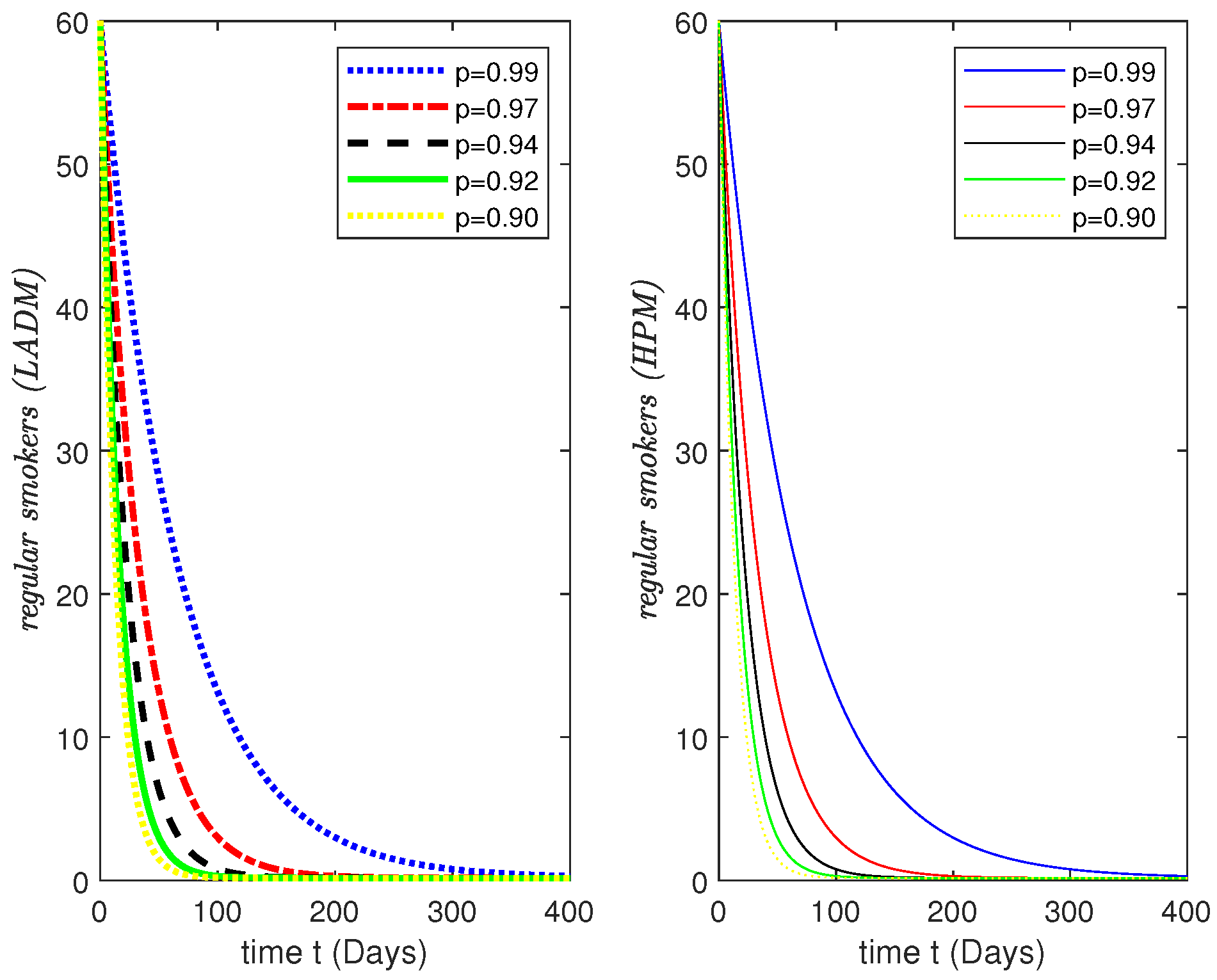
4. Simulations Results and Discussion

We offer numerical simulation for the proposed model to allow for the variation of our semi-analytical findings in both ways. The simulation makes use of qualitative point analysis and takes into account the parameters from a biological feasibility aspect. The starting class sizes for each compartment, namely, Susceptible $X\left(t\right)$, Snuffing $H\left(t\right)$, Irregular $J\left(t\right)$, Regular $Y\left(t\right)$, and quitter $Z\left(t\right)$, are taken from the Section 3.2 together with the numerical values of the parameters. In this section graph of all five compartments is signified, and the explanation of the behavior of all the classes is discussed. Moreover, the results are shown in Figure 1, Figure 2, Figure 3, Figure 4 and Figure 5.

The dynamical behavior of the susceptible class $X\left(t\right)$ is depicted in Figure 1 at different fractional orders. For the lower fractional order, the drop is noticeable, while for the higher fractional order, it is less noticeable. Furthermore, after 250 days, it becomes approximately constant. Figure 2 presents the behavior of the snuffing class $H\left(t\right)$ at various fractional orders. It grows at high fractional order and for low fractional order, it grows first and then going to decrease after 150 days.

In Figure 3, the irregular class $J\left(t\right)$ grows rapidly for low fractional order and then grows slowly for high fractional order. The dynamical behavior of regular class $Y\left(t\right)$ is shown in Figure 4. The results show that for the lower fractional order, the drop is remarkable, while for the higher order, it is less remarkable.

Similarly, Figure 5 shows that the growth in quitter class $Z\left(t\right)$ grows rapidly for low fractional order and grows slowly for high fractional order.

In the next figure, Figure 6, we present the dynamical behavior of the five compartments of the considered model by taking different values for the initial conditions along with the same fractional orders.

Next, we are intended to present a comparison of the numerical solutions of distinct compartments of the studied model via both the suggested method of HPM and LADM for the first few terms that display simulation similarities as given from Figure 7, Figure 8, Figure 9, Figure 10 and Figure 11.

Figure 7, Figure 8, Figure 9, Figure 10 and Figure 11 show the comparison of the numerical simulations of the solutions of all the compartments of the considered model. Furthermore, it is noted that both the techniques LADM and HPM have the same results, so the graphical representation is also the same for each compartment. The susceptible class $X\left(t\right)$ and the regular smokers class $Y\left(t\right)$ are decreasing with time, the snuffing class $H\left(t\right)$ first increases with time and then decreases after some time, and the irregular smokers class $J\left(t\right)$ are rapidly increasing over time.

Moreover, the below Figure 12, Figure 13, Figure 14, Figure 15 and Figure 16 present the comparison of LADM and HPM by taking different values of the initial conditions but having the same fractional order values.

5. Conclusions

In this paper, the dynamical behavior of the smoking mathematical model via the Caputo-Fabrizio differential operator is analyzed and makes use of the utilities of fractional calculus. The considered model has been numerically explored by employing the Homotopy perturbation method (HPM) and the Laplace transform with the Adomian decomposition method (LADM). The numerical results obtained with the hired methods are significantly identical and have provided the finest confirmation for the considered model in arbitrary order derivatives. The outcomes are influenced by various parameters used in the considered model. Both methods converge and are useful for solving nonlinear fractional order differential equations. It is also important to emphasize that, when compared to standard methods, the method can save processing effort while maintaining good numerical accuracy. Moreover, the numerical simulation results of the underlying problem have been facilitated with the aid of Matlab, and the graphical behavior of each compartment of the considered problem at arbitrary order derivatives has been presented. From the presented simulation, we conclude that fractional order systems reveal more prosperous dynamics than the one with the integer order. As well, we anticipate that the existing study will be more beneficial in the account of smoking matter thinking of determination and education. Conceivably, in the future, the gained elements may lead us to do more research on this subject. For example, the mathematical model can be modernized by considering various dynamical structures and can be investigated with different types of derivatives.

References

1. Brownlee, J. Certain considerations on the causation and course of epidemics. Proc. R. Soc. Med. 1909, 2, 243–258. [Google Scholar] [CrossRef] [PubMed]
2. Brownlee, J. The mathematical theory of random migration and epidemic distribution. Proc. R. Soc. Edinb. 1912, 31, 262–289. [Google Scholar] [CrossRef]
3. Kermack, W.O.; McKendrick, A.G. Contributions to the mathematical theory of epidemics. part 1. Proc. R. Soc. Edinb. Sect. A Math. 1927, 115, 700–721. [Google Scholar]
4. Chong, J.R. Analysis clarifies route of AIDS. Los Angeles Times, 30 October 2000. [Google Scholar]
5. Wang, K.; Wang, W.; Song, S. Dynamics of an HBV model with difusion and deley. J. Theor. Biol. 2008, 253, 36–44. [Google Scholar] [CrossRef] [PubMed]
6. McCluskey, C.C. Complete global stability for an SIR epidemic model with delay distributed or discrete. Nonlinear Anal. Real World Appl. 2010, 11, 55–59. [Google Scholar] [CrossRef]
7. Xu, R.; Ma, Z. Stability of a delayed SIRS epidemic model with a nonlinear incidence rate. Chaos Solitons Fractals 2009, 41, 2319–2325. [Google Scholar] [CrossRef]
8. Leone, A.; Landini, L.; Leone, A. What is tobacco smoke? Sociocultural dimensions of the association with cardiovascular risk. Curr. Pharm. Des. 2010, 16, 2510–2517. [Google Scholar] [CrossRef]
9. Saha, S.P.; Bhalla, D.K.; Whayne, T.F.; Gairola, C.G. Cigarette smoke and adverse health effects: An overview of research trends and future needs. Int. J. Angiol. 2007, 16, 77–83. [Google Scholar] [CrossRef] [Green Version]
10. Smith, E.A.; Malone, R.E. Everywhere the soldier will be, wartime tobacco promotion in the US military. Am. J. Publ. Health 2009, 99, 1595–1602. [Google Scholar] [CrossRef]
11. Costa, R.M.S.; Pavone, P. Diachronic biodiversity analysis of a metropolitan area in the Mediterranean region. Acta Hortic. 2018, 1215, 49–52. [Google Scholar] [CrossRef]
12. Costa, R.M.S.; Avone, P. Invasive plants and natural habitats: The role of alien species in the urban vegetation. Acta Hortic. 2018, 1215, 57–60. [Google Scholar] [CrossRef]
13. Sharomi, O.; Gumel, A.B. Curtailing smoking dynamics: A mathematical modeling approach. Appl. Math. Comput. 2008, 195, 475–499. [Google Scholar] [CrossRef]
14. Liu, T.; Deiss, T.J.; Lippi, M.W.; Jauregui, A.; Vessel, K.; Ke, S.; Belzer, A.; Zhuo, H.; Kangelaris, K.N.; Gomez, A.D.; et al. Alternative Tobacco Product Use in Critically Ill Patients. Int. J. Environ. Res. Public Health 2020, 17, 8707. [Google Scholar] [CrossRef]
15. Gerrits, N.; Elen, B.; Craenendonck, T.V.; Triantafyllidou, D.; Petropoulos, I.N.; Malik, R.A.; De Boever, P. Age and sex affect deep learning prediction of cardiometabolic risk factors from retinal images. Sci. Rep. 2020, 10, 9432. [Google Scholar]
16. Yildirum, A.; Cherruault, Y. Analytical approximate solution of a SIR epidemic model with constant vaccination strategy by homotopy perturbation method. Emerald 2009, 38, 1566–1581. [Google Scholar]
17. World Health Organisation. Monitoring Tobacco Use and Prevention Policies. Executive Summary; World Health Organisation: Geneva, Switzerland, 2017.
18. Goldenberg, I.; Jonas, M.; Tenenbaum, A.; Boyko, V.; Matetzky, S.; Shotan, A.; Behar, S.; Reicher-Reiss, H.; Bezafibrate Infarction Prevention Study Group. Current smoking, smoking cessation, and the risk of sudden cardiac death in patients with coronary artery disease. Arch. Int. Med. 2003, 163, 2301–2305. [Google Scholar] [CrossRef]
19. Castillo-Garsow, C.; Jordan-Salivia, G.; Rodriguez Herrera, A. Mathematical Models for Dynamics of Tobacco Use, Recovery and Relapse; Technical Report Series BU-1505-M; Cornell University: London, UK, 2000. [Google Scholar]
20. Ham, O.K. Stages and processes of smoking cessation among adolescents. West. J. Nurs. Res. 2007, 29, 301–315. [Google Scholar]
21. Zaman, G. Qualitative behavior of giving up smoking models. Bull. Malays. Math. Soc. 2011, 34, 403–415. [Google Scholar]
22. Erturk, V.S.; Zaman, G.; Momani, S. A numeric analytic method for approximating a giving up smoking model containing fractional derivatives. Comput. Math. Appl. 2012, 64, 3068–3074. [Google Scholar] [CrossRef] [Green Version]
23. Zeb, A.; Chohan, I.; Zaman, G. The homotopy analysis method for approximating of giving up smoking model in fractional order. Appl. Math. 2012, 3, 914–919. [Google Scholar] [CrossRef]
24. Alkhudhari, Z.; Al-Sheikh, S.; Al-Tuwairqi, S. Global dynamics of a mathematical model on smoking. Appl. Math. 2014, 2014, 847075. [Google Scholar] [CrossRef]
25. Khalid, M.; Khan, F.S.; Iqbal, A. Perturbation-iteration algorithm to solve fractional giving up smoking mathematical model. Int. J. Comput. Appl. 2016, 142, 1–6. [Google Scholar] [CrossRef]
26. Kilbas, A.A.; Srivastava, H.M.; Trujillo, J.J. Theory and Applications of Fractional Differential Equations; Elsevier: Amsterdam, The Netherlands, 2006; Volume 204. [Google Scholar]
27. Diethelm, K.; Garrappa, R.; Stynes, M. Good (and not so good) practices in computational methods for fractional calculus. Mathematics 2020, 8, 324. [Google Scholar] [CrossRef] [Green Version]
28. Salnikov, N.N.; Siryk, S.V.; Tereshchenko, I.A. On Construction of finite dimensional mathematical model of convection diffusion process with usage of the Petrov Galerkin method. J. Autom. Inf. Sci. 2010, 42, 67–83. [Google Scholar] [CrossRef]
29. Roos, H.G.; Stynes, M.; Tobiska, L. Robust Numerical Methods for Singularly Perturbed Differential Equations: Convection-Diffusion-Reaction and Flow Problems; Springer Science & Business Media: Berlin/Heidelberg, Germany, 2008; Volume 24. [Google Scholar]
30. Stynes, M.; Stynes, D. Convection-Diffusion Problems; American Mathematical Society: Providence, RI, USA, 2018; Volume 196. [Google Scholar]
31. Siryk, S.V. Accuracy and stability of the Petrov–Galerkin method for solving the stationary convection-diffusion equation. Cybern. Syst. Anal. 2014, 50, 278–287. [Google Scholar] [CrossRef]
32. Siryk, S.V. Analysis of lumped approximations in the finite-element method for convection–diffusion problems. Cybern. Syst. Anal. 2013, 49, 774–784. [Google Scholar] [CrossRef]
33. Saadatmandi, A.; Dehghan, M. A new operational matrix for solving fractional-order differential equations. Comput. Math. Appl. 2010, 59, 1326–1336. [Google Scholar] [CrossRef] [Green Version]
34. Caputo, M.; Fabrizio, M. Applications of new time and spatial fractional derivatives with exponential kernels. Prog. Frac. Diff. Appl. 2016, 2, 1–11. [Google Scholar] [CrossRef]
35. El-Saka, H.A.A. The fractional-order SIS epidemic model with variable population size. J. Egyp. Math. Soc. 2014, 22, 50–54. [Google Scholar] [CrossRef] [Green Version]
36. Caponetto, R. Fractional Order Systems: Modeling and Control Applications; World Scientific: Singapore, 2010; Volume 72. [Google Scholar]
37. Ma, T.; Sun, N. Zhiliang Wang, Dongsheng Yang. Nonlinear Dyn. 2014, 75, 387–402. [Google Scholar]
38. Kazem, S.; Abbasbandy, S.; Kumar, S. Fractional-order Legendre functions for solving fractional-order differential equations. Appl. Math. Model. 2013, 37, 5498–5510. [Google Scholar] [CrossRef]
39. Podlubny, I. Fractional differential equations. Math. Sci. Eng. 1999, 198, 41–119. [Google Scholar]
40. Kilbas, A.A.; Trujillo, J.J. Differential equations of fractional order: Methods results and problem—I. Appl. Anal. 2001, 78, 153–192. [Google Scholar] [CrossRef]
41. Liu, X.; ur Rahmamn, M.; Ahmad, S.; Baleanu, D.; Nadeem Anjam, Y. A new fractional infectious disease model under the non-singular Mittag–Leffler derivative. Waves Random Complex Media 2022, 1–27. [Google Scholar] [CrossRef]
42. ur Rahman, M.; Arfan, M.; Shah, Z.; Alzahrani, E. Evolution of fractional mathematical model for drinking under Atangana-Baleanu Caputo derivatives. Phys. Scr. 2021, 96, 115203. [Google Scholar] [CrossRef]
43. Xu, C.; ur Rahman, M.; Baleanu, D. On fractional-order symmetric oscillator with offset-boosting control. Nonlinear Anal. Model. Cont. 2022, 27, 994–1008. [Google Scholar] [CrossRef]
44. Caputo, M. Elasticita e Dissipazione; Zanichelli: Bologna, Italy, 1969. [Google Scholar]
45. Caputo, M.; Fabrizio, M. On the singular kernels for fractional derivatives. Some applications to partial differential equations. Progr. Fract. Differ. Appl. 2021, 7, 1–4. [Google Scholar]
46. Caputo, M.; Fabrizio, M. A new definition of fractional derivative without singular kernel. Prog. Fract. Differ. Appl. 2015, 1, 73–85. [Google Scholar]
47. Losada, J.; Nieto, J.J. Properties of the new fractional derivative without singular kernel. Prog. Fract. Differ. Appl. 2015, 1, 87–92. [Google Scholar]
48. Bai, C.Z.; Fang, J.X. The existence of a positive solution for a singular coupled system of nonlinear fractional differential equations. Appl. Math. Comput. 2004, 150, 611–621. [Google Scholar] [CrossRef]
49. Haq, F.; Shah, K.; Rahman, G.U.; Shahzad, M. Numerical analysis of fractional order model of HIV-1 infection of CD4+ T-cells. Comput. Meth. Diff. Equ. 2017, 5, 1–11. [Google Scholar]
50. Biazar, J. Solution of the epidemic model by Adomian decomposition method. Appl. Math. Comput. 2006, 173, 1101–1106. [Google Scholar] [CrossRef]
51. He, J.H. An elementary introduction to the homotopy perturbation method. Comput. Math. Appl. 2009, 57, 410–412. [Google Scholar] [CrossRef] [Green Version]
52. Ahmad, S.; Ullah, A.; Akgül, A.; De la Sen, M. A novel homotopy perturbation method with applications to nonlinear fractional order KdV and Burger equation with exponential-decay kernel. J. Funct. Spaces 2021, 2021, 8770488. [Google Scholar] [CrossRef]
53. Sun, H.; Zhang, Y.; Baleanu, D.; Chen, W.; Chen, Y. A new collection of real world applications of fractional calculus in science and engineering. Commun. Nonlinear Sci. Numer. Simul. 2018, 64, 213–231. [Google Scholar] [CrossRef]
54. Xu, Y. Similarity solution and heat transfer characteristics for a class of nonlinear convection-diffusion equation with initial value conditions. Math. Probl. Eng. 2019, 2019, 3467276. [Google Scholar] [CrossRef]
55. Miller, K.S.; Ross, B. An Introduction to the Fractional Calculus and Fractional Differential Equations; Wiley: Hoboken, NJ, USA, 1993. [Google Scholar]
56. Nchama, G.A.M.; Mecıas, A.L.; Richard, M.R. The Caputo–Fabrizio fractional integral to generate some new inequalities. Inf. Sci. Lett. 2019, 8, 73–80. [Google Scholar]
57. He, J.H.; Jiao, M.L.; Gepreel, K.A.; Khan, Y. Homotopy perturbation method for strongly nonlinear oscillators. Math. Comput. Simul. 2023, 204, 243–258. [Google Scholar] [CrossRef]
58. He, J.H. A tutorial review on fractal spacetime and fractional calculus. Int. J. Theor. Phys. 2014, 53, 3698–3718. [Google Scholar] [CrossRef]
Figure 1. Adaptive nature of the approximated result for the susceptible class X ( t ) class of the considered model at different arbitrary fractional orders.
Fractalfract 06 00623 g001
Figure 2. Adaptive nature of the approximated result for the snuffing class H ( t ) class of the proposed model at different arbitrary fractional orders.
Fractalfract 06 00623 g002
Figure 3. Adaptive nature of the approximated result for the irregular smokers J ( t ) class of the considered model at different arbitrary fractional orders.
Fractalfract 06 00623 g003
Figure 4. Adaptive nature of the approximated result for the regular smokers Y ( t ) class of the proposed model at different arbitrary fractional orders.
Fractalfract 06 00623 g004
Figure 5. Adaptive nature of the approximated result for the quitter smokers Z ( t ) class of the considered model at different arbitrary fractional orders.
Fractalfract 06 00623 g005
Figure 6. Fractional dynamical behavior of all the compartments of the considered model having different initial conditions along with the same fractional orders. (a) Dynamical behavior of class X ( t ) at t = 150 ; (b) Dynamical behavior of class H ( t ) at t = 100 ; (c) Dynamical behavior of class J ( t ) at t = 80 ; (d) Dynamical behavior of class Y ( t ) at t = 60 ; (e) Dynamical behavior of class X ( t ) at t = 40 .
Fractalfract 06 00623 g006aFractalfract 06 00623 g006b
Figure 7. Comparison of the approximate solution for X ( t ) class of the suggested model at different arbitrary fractional orders by LADM and HPM.
Fractalfract 06 00623 g007
Figure 8. Comparison of the approximate solution for H ( t ) class of the proposed model at different arbitrary fractional orders by LADM and HPM.
Fractalfract 06 00623 g008
Figure 9. Comparison of the approximate solution for J ( t ) class of the proposed model at different arbitrary fractional orders by LADM and HPM.
Fractalfract 06 00623 g009
Figure 10. Comparison of the approximate solution for Y ( t ) class of the suggested model at different arbitrary fractional orders by LADM and HPM.
Fractalfract 06 00623 g010
Figure 11. Comparison of the approximate solution for Z ( t ) class of the proposed model at different arbitrary fractional orders by LADM and HPM.
Fractalfract 06 00623 g011
Figure 12. Comparison of the approximate solution for X ( t ) class of the proposed model having initial condition 150.
Fractalfract 06 00623 g012
Figure 13. Comparison of the approximate solution for H ( t ) class of the proposed model having initial condition 100.
Fractalfract 06 00623 g013
Figure 14. Comparison of the approximate solution for J ( t ) class of the proposed model having initial condition 80.
Fractalfract 06 00623 g014
Figure 15. Comparison of the approximate solution for Y ( t ) class of the proposed model having initial condition 60.
Fractalfract 06 00623 g015
Figure 16. Comparison of the approximate solution for Z ( t ) class of the proposed model having initial condition 40.
Fractalfract 06 00623 g016