Abstract
To obtain high-quality Pareto optimal solutions and to enhance the searchability of the biogeography-based optimization (BBO) algorithm, we present an improved BBO algorithm based on hybrid migration and a dual-mode mutation strategy (HDBBO). We first adopted a more scientific nonlinear hyperbolic tangent mobility model instead of the conventional linear migration model which can obtain a solution closer to the global minimum of the function. We developed an improved hybrid migration operation containing a micro disturbance factor, which has the benefit of strengthening the global search ability of the algorithm. Then, we used the piecewise application of Gaussian mutation and BBO mutation to ensure that the solution set after mutation was also maintained at a high level, which helps strengthen the algorithm’s search accuracy. Finally, we performed a convergence analysis on the improved BBO algorithm and experimental research based on 11 benchmark functions. The simulation results showed that the improved BBO algorithm had superior advantages in terms of optimization accuracy and convergence speed, which showed the feasibility of the improved strategy.
1. Introduction
A multitude of optimization algorithms inspired by biological phenomena and laws have been established. Over the past decades, many algorithms have been widely used to solve problems concerning multi-objective programming engineering, and in other research fields [1,2] several other classical algorithms have been used, including differential evolution (DE), particle swarm optimization (PSO), the genetic algorithm (GA), and the sparrow search algorithm (SSA). However, recent theoretical developments have revealed that the BBO algorithm is more efficient in solving such problems. The BBO algorithm was first proposed by Simon in 2008 and is similar to most other optimization algorithms inspired by biogeography theory. The algorithm has a simple principle and few parameters; the well-known disadvantages of the BBO algorithm are that it easily falls into local optimization and slowly converges in a complex running environment. Therefore, research on the theory and application of the BBO algorithm is of high academic and engineering value [3,4,5].
Many scholars have maintained high enthusiasm for researching and improving the BBO algorithm in recent years. The studies conducted on the BBO algorithm can be divided into the following three groups after consulting the data and summarizing them: Firstly, theoretical analyses are carried out on the basis of various BBO algorithm models. Simon [6] applied the Markov chain model to research the BBO algorithm’s global convergence, and the results indicated that many influencing factors gave rise to the algorithm, such as population size, migration model, and initial immigration. Ma et al. [7] established four different mobility models according to the species distribution in the biogeography literature, which was important for further studies. Parimal et al. [8] proposed a novel migration model and an adaptive local topological structure for the algorithm. In summary, little in-depth research has been conducted on the theory of the BBO algorithm at present, and most scholars mainly illustrate the performance of the improved BBO algorithm with simulation results. Secondly, researchers have mainly focused on strategies to optimize the BBO algorithm, which included improving the algorithm operator or referring to strategies for improving other algorithms. Sayyed et al. [9] combined the BBO algorithm with the PSO algorithm to establish a novel hybrid metaheuristic method. Zhang et al. [10] proposed an improved BBO algorithm by adding a differential mutation operator to the migration operation and increasing the migratory number. In addition, Zhao et al. [11] developed an excellent migration strategy, whereby the constant and sinusoidal migration models are used in the early and late iterative stages, respectively. Santosh et al. [12] proposed an improved hybrid method based on the combination of the BBO algorithm and the recursive least square (RLS) algorithm. Finally, according to the remaining studies, the improved BBO algorithm was employed for various optimization issues. He et al. [13] presented an improved BBO algorithm based on the elite learning (EL) strategy and applied it to solve complex problems related to multimodal medical image registration. Furthermore, Zhang et al. [14] developed an improved BBO algorithm that could effectively resolve the manufacturing service supply chain optimization (MSSCO) problem. Amin [15] used the BBO algorithm to establish an improved method for optimizing plate-fin heat exchangers. Liu et al. [16] applied the BBO algorithm to the design of power grid partitions, and the results demonstrated that the method of the power grid community network is reasonable to a certain extent. Furthermore, Zhang et al. [17] developed a heuristic approach based on the BBO algorithm to solve the multistage multiproduct scheduling problem (MMSP) in a rational amount of time.
Based on the above literature, although the performance of the BBO algorithm has been strengthened from different aspects and has achieved certain positive results, due to the diversity and complexity of different research problems, further improvement of the algorithm in terms of optimization accuracy, convergence speed, and stability is desired. In this paper, we propose an improved BBO algorithm based on hybrid migration and dual-mode mutation. The hybrid migration contributes to enhancing the global search capability of the algorithm and the Gaussian and BBO variations enhance the search accuracy of the algorithm. The remainder of this paper is structured as follows: In Section 2, we develop three improvement strategies and study their feasibility. In Section 3, we provide the simulation results, and then we compare and study the performance of the improved BBO algorithm and other algorithms. Section 4 is the conclusion with discussions of future work.
2. Improved BBO Algorithm and Strategies
2.1. HDBBO Algorithm
The core operation of the BBO algorithm is to simulate the migration and mutation of biological populations [18]. Among them, the migration operation is designed to facilitate information sharing. The migration of each species’ habitat is shown in Figure 1, where H1 denotes the first population habitat (H2 denotes the second population habitat,…, Hi+1 denotes the i + 1th population habitat) which can receive species from H2 and H6, while some species in this habitat emigrate to H7. In addition, we used the mutation operation to scientifically simulate the possible species variation caused by a change in the environment of the habitats. Furthermore, Table 1 shows the correspondence between the BBO algorithm and biogeography theory [19].
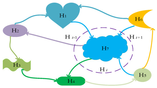
Figure 1.
Diagram of species migration between habitats.

Table 1.
Correspondence between BBO algorithm and biogeography theory.
The improved BBO algorithm is called the HDBBO algorithm because it involves hybrid migration and dual-mode mutation. The flowchart of the HDBBO algorithm is shown in Figure 2.
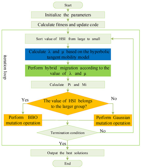
Figure 2.
HDBBO algorithm flow chart.
The improvements in the HDBBO algorithm can be summarized as follows: First, the HDBBO algorithm obtains the HSI through the initialization parameter calculation and updates the HSI, sorting the HSI from large to small. In the migration model section, the HDBBO algorithm uses the hyperbolic tangent mobility model to calculate the in-migration and out-migration rates instead of the traditional linear mobility model. It performs the mixed species migration operation using Equation (3) based on the values of the in-migration and out-migration rates. Then, it calculates the habitat species probability and mutation rate. Furthermore, it judges whether the HSI value belongs to a larger group, if so, it adopts the BBO variation; otherwise, it adopts the Gaussian variation. Finally, it judges the termination condition of the obtained results. If the results are to be terminated, it obtains the optimal solution; otherwise, it performs the iterative cyclic calculation. Details on the reasonability and applicability of these three improvement strategies are further discussed in later sections.
2.2. Hyperbolic Tangent Mobility Model
The BBO algorithm uses the linear migration model to describe the immigration and emigration of species in habitats. After years of research and development, scholars have only proposed a few novel migration models based on the exponential, quadratic, and cosine functions. Additionally, researchers have repeatedly executed studies based on nonlinear migration models. After repeated comparisons, the HDBBO algorithm adopts the hyperbolic tangent mobility model, which is shown in Figure 3.
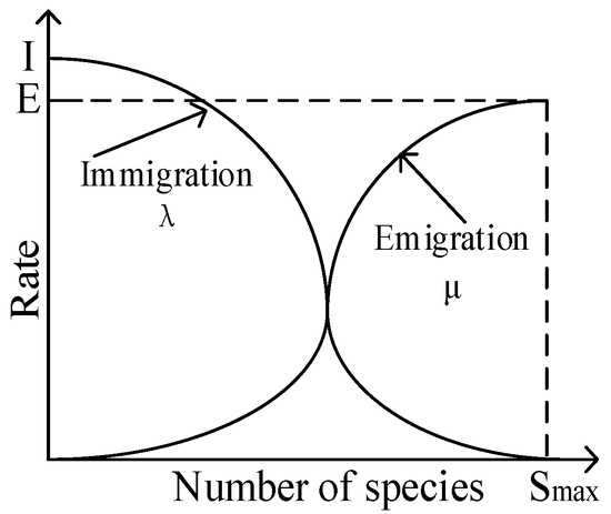
Figure 3.
Hyperbolic tangent mobility model of species.
As shown in Figure 3, we established the relationship between the number of species and migratory rate in a habitat, and the migratory rate is composed of the immigratory rate and emigratory rate . As indicated in Figure 3, when the number of species in the habitat is , the maximum immigratory rate is and the emigratory rate is . In contrast, the immigratory rate is and the maximum emigratory rate is when the number of species reaches the maximum . Furthermore, when fewer or more species are present in the habitat, the change in the migratory rate tends to be gentle. Additionally, the variation is greater and more evident when the number fluctuates within a certain range. Therefore, this nonlinear relationship is exceedingly consistent with biogeography theory, and the migratory rate based on the hyperbolic tangent mobility model can be expressed by Equations (1) and (2). The value of is usually set to [20]. In the hyperbolic tangent mobility model, is usually meaningless; however, the smaller the value, the more relaxed the curve, and the closer the model to the actual law. Thus, in this paper, the experimental results suggested that the improved BBO algorithm works more effectively when .
where and , represent the immigratory and emigratory rate, respectively, when the number of species in the habitat is ; and represent the maximum values of the immigratory and emigratory rates, respectively; is the impact factor parameter; and represent the current and maximum number of species, respectively.
2.3. Hybrid Migration Operation
Most scholars have been committed to improving the migratory operator to enhance the performance of the BBO algorithm [21,22]. However, an improved hybrid migration strategy including a perturbation factor was developed, which could be described as follows: According to the migratory rate value, if a certain SIV of must change to adapt the environment, where represents the habitat, and are combined with a micro disturbance factor to achieve the hybrid migration operation. Consequently, the expression of this improved hybrid migration strategy is given by:
where represents the micro disturbance factor; is the suitable index vector; and represent the corresponding SIVs, which are desired to immigrate or emigrate between habitats; and denote the current and maximum iterative number, respectively; represents a random number in the to range.
and are defaulted when no iteration occurs in the study, and the discrete migration operation is realized in habitats, which can be shown as . Currently, most of the high-quality SIVs of can be obtained by , and the HDBBO algorithm maintains a strong global exploration ability.
Then, the HDBBO algorithm starts to iterate, is smaller at the beginning of the iterations, and is a constant. Consequently, the ratio of to is smaller, which causes the value of the sine function to be small with a rapid change in the ratio with increasing numbers of iterations. Accordingly, the value of gradually decreases from one with a higher speed. Nonetheless, the value of is generally larger in this iterative phase and a wide search range from to is produced. Numerous high-quality suitable index vectors may be transferred among habitats to share the information, which facilitates the increase in biological population diversity. Thus, in this process, the global optimization ability of the HDBBO algorithm gradually decreases, while the local optimization ability accordingly strengthens.
Similarly, in the middle and late iterative stage of the algorithm, becomes larger, but the reduction speed of the value slowly decreases due to the existence of the sine function. As expected, the local optimization ability continues to increase, while the global optimization ability gradually decreases. When , the SIV can satisfy the survival requirements of most species and the HSI is exceedingly high. This suggests almost no migration operation occurs in the habitats and the dynamic balance state is established. Therefore, the local high-quality SIV can be maintained.
In general, . Due to the sinusoidal function including the number of iterations, the value of becomes more flexible. Consequently, compared with the BBO algorithm, the improved hybrid migration strategy considers both the global and local optimization abilities and it increases the optimization accuracy of the HDBBO algorithm.
Algorithm 1 presents the pseudo code of the hybrid migration strategy.
| Algorithm 1 Hybrid Migration Strategy. |
| 1: Parameter:, , , , |
| 2: Initialization: Generate habitats as size as population size; |
| 3: Population evaluation: Evaluate habitats |
| 4: for : Population size |
| 5: for : Feature dimension |
| 6: if , then // Determine whether immigrates by |
| 7: Select the that is considered as immigrating; |
| 8: end |
| 9: if , then // Determine whether immigrates by |
| 10: Select the that is regarded as emigrating |
| 11: end |
| 12: Realize hybrid migration and update according to Equation (3). |
| 13: end |
2.4. Dual-Mode Mutation Operation
Sudden changes in temperature, infectious diseases, drought, and flood often occur in habitats, which have a substantial impact on the survival of organisms. Based on this phenomenon, we designed the mutation operator in the BBO algorithm. Many studies have demonstrated that the HSI changes with these disasters. The fewer or more species that a habitat contains, the higher its mutation probability, with the habitats in the steady state nearly always being less affected. Therefore, the lower the occurrence probability of the species contained in the habitat, the more prone the algorithm is to mutation operations. To be precise, the mutational rate , which is inversely proportional to , can be calculated with
where is the maximum mutation rate, which can be defined by scholars, , and represents the probability that the habitat contains species; furthermore, is given with and by
In essence, the result of the mutation operation of the conventional BBO algorithm is indeterminate (it either enhances or diminishes performance). In other words, the findings are equivalent to replacing the SIV of the original habitat with another SIV randomly selected within a certain range. A basic BBO mutation has the advantage of generating various solutions and facilitating the diversity of the SIV. However, an excellent SIV may be destroyed, and scholars are uncertain if the SIV after mutation can be applied to the entire solution set, which ultimately affects the convergence speed of the algorithm. Therefore, several improved methods for mutation operators have been proposed to reduce the impact of the basic BBO mutation [23,24].
In this study, we introduced and combined Gaussian mutation with BBO mutation, and the HDBBO algorithm uses these two disparate mutational methods. The probability density function of the Gaussian mutation is shown in Equation (6):
where represents the average value and denotes the variance. In addition, is the quintessential Gaussian distribution, as .
When Gaussian mutation is implemented, 12 random numbers from to are assumed to be present, and they are presumed to be evenly distributed; then, a random number conforming to can be calculated by
The Gaussian mutation operation process can be described as follows: When the Gaussian mutation from the to the of the species is accomplished, the mutation point expression () can be shown as
where and represent the SIV of before and after Gaussian mutation, respectively.
The HDBBO algorithm initially sorts the HSI of the habitats from high to low. The algorithm uses the basic BBO mutation for the habitats with a higher HSI. The use of this strategy can result in an increased population diversity in a certain range and a high-quality SIV being retained after mutation. In contrast, Gaussian mutation is applied to the habitats that possess a lower HSI. In the later iterations of the HDBBO algorithm, is approximated to , and the accurate SIV search in the local range is facilitated by the high capability of Gaussian mutation, which is able to reduce the influence of the inferior solution on the entire solution set and enhance the HDBBO algorithm’s performance.
The pseudo code of the dual-mode mutation operation is demonstrated in Algorithm 2.
| Algorithm 2 Dual-mode Mutation Operation |
| 1: Sort the population according to the HSI of the habitats from high to low |
| 2: for : Population size |
| 3: for : Feature dimension |
| 4: if , then; |
| 5: The basic BBO mutation is used in habitats with higher HSI; |
| 6: else |
| 7: Gaussian mutation is used in habitats with lower HSI according to Equation (8). |
| 8: end |
| 9: end |
3. Simulations and Discussion
To verify whether the performance of the HDBBO algorithm was enhanced and to further judge the feasibility of the improvement measures, we implemented a multitude of experimental simulations on 11 benchmark functions with different complexities. We divided the experiments into two parts. In the first half, we compared the ideal function solutions obtained by the HDBBO algorithm and two other classical algorithms. In the second half, we studied the influence of different values of , where represents the impact factor parameter regarding the migratory rate.
3.1. Selection of Benchmark Functions
We selected 11 quintessential benchmark functions to test the performance of these three algorithms, and the relevant descriptions of these functions are shown in Table 2. We found that are unimodality functions, which we used to test the convergence characteristics of each algorithm. In contrast, are all multimodality functions, which we mainly used to test the algorithms’ ability to avoid falling into local ideal solutions. The 11 functions chosen were all complex nonlinear classical test functions, which were appropriate for accurately and objectively appraising the overall performance of the algorithms.

Table 2.
Test performance function features.
3.2. Parameters Setting
We used MATLAB (Version: R2018b) as the programming language to complete the simulation experiments. The relevant parameters that were set in MATLAB were as follows: the population size was set to , the dimension of these functions was defined as , the global migration rate was one, the maximum values of and were assumed to be one, the values of the maximum mutation rate and Gaussian mutation rate were , and the maximum number of iterations was set to . To avoid the contingency of the results and to ensure the universality of the experimental conclusions, we set the three algorithms to independently run times on each test function.
3.3. Analysis of the Simulation Results
3.3.1. Comparison of Different Algorithms
As Gaussian mutation is similarly involved in the improved strategy of the BBO algorithm, the proposed improved algorithm is called the GBBO algorithm [25]. To demonstrate the superiority of the HDBBO algorithm compared with the conventional BBO and GBBO algorithms, we carried out experiments under the same running environment and parameters. We defined in this group of experiments, and the influence of different values on the HDBBO algorithm was determined in the next group of experiments. Based on these conditions, the comparison results of 11 benchmark functions are shown in Table 3.

Table 3.
Simulation data of three algorithms on 11 benchmark functions.
In this study we used three indexes, the average value, the best value, and the standard deviation (Std) of the test functions to compare the capability of the three algorithms. Specifically, the average value represents the mean solution of each benchmark function, which roughly reflects the applicability of an algorithm to diverse test functions and its optimization accuracy. Furthermore, the best value denotes the ideal solution solved by each algorithm, which demonstrates the ability of the algorithm to seek the global optimal value. Furthermore, the standard deviation reflects the distribution of the Pareto optimal solution and intuitively demonstrates the overall performance of the algorithms.
According to the results shown in Table 3, which we obtained from the analysis of the three evaluation criteria of the three algorithms under the same operating environment and parameters, the HDBBO algorithm invariably possesses advantages regardless of the unimodal function or multimodal function. We noticed that the functions calculated by the HDBBO algorithm were nearly always relatively small and the results were more approximate to the optimal solution of the test functions. Indeed, for the functions of , , and , the best solutions all reached zero, which demonstrates the excellent capability of the HDBBO algorithm. Furthermore, Figure 4 shows the convergence curves of the three algorithms on different benchmark functions, which we created to accurately and objectively evaluate these algorithms and are intuitively indicative of the experimental results.
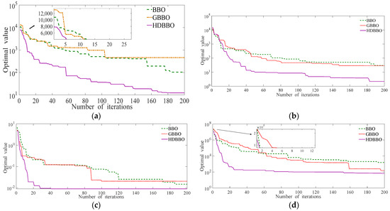
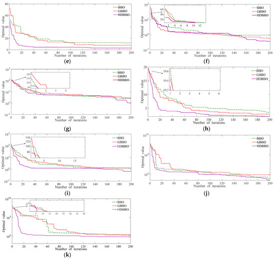
Figure 4.
Comparison of the three algorithms on 11 benchmark functions (a–k) on the convergence of −.(a) convergence of the three algorithms on benchmark function ; (b) convergence of the three algorithms on benchmark function ; (c) convergence of the three algorithms on benchmark function ; (d) convergence of the three algorithms on benchmark function ; (e) convergence of the three algorithms on benchmark function ; (f) convergence of the three algorithms on benchmark function ; (g) convergence of the three algorithms on benchmark function ; (h) convergence of the three algorithms on benchmark function ; (i) convergence of the three algorithms on benchmark function ; (j) convergence of the three algorithms on benchmark function ; (k) convergence of the three algorithms on benchmark function .
Figure 4 shows that the abscissa axis represents the iterative number of each test function and the ordinate axis represents the best value of each test function optimized by the three algorithms. Due to the different attributes of each test function, the optimal value resolved by the algorithms varies in the magnitude order. For easy observation, we linearly expressed the best and values, while we expressed the others on a based 10 logarithm. To expediently identify the numerical difference at the beginning of the iterations, we created partial enlarged diagrams of the parts of the functions, which was essential in comparing the capabilities of the algorithms.
We had the following discussion through the comparison and research concerning Figure 4. For the , , , and functions, at the initial stage of the iterations, the HDBBO algorithm produced a more optimal value than the other two algorithms. Therefore, the improved strategies that were proposed did not reduce the capabilities of the algorithm. Conversely, the optimization ability of the algorithm could be enhanced to a certain extent, and the superior applicability of the HDBBO algorithm could be demonstrated. Furthermore, the search speed of the BBO algorithm and GBBO algorithm considerably slowed in the middle and late iterations, and these two algorithms tended to fall into local optimization after the iteration. Nevertheless, the convergence curve of the HDBBO algorithm was almost vertical at the beginning of the iterative stage because of the algorithm’s strong exploration ability. Moreover, the global optimization solution was almost achieved when the iteration number was , thus explaining the excellent data development ability of the improved BBO algorithm. In addition, although each algorithm was independently running and their operating environments were identical, the best value of the functions could have been invariably obtained by the improved BBO algorithm with a faster speed, which implies that the computational complexity of the HDBBO algorithm is small. Furthermore, the distribution of the Pareto optimal solution suggested that the HDBBO algorithm was stable.
3.3.2. Further Research on HDBBO Algorithm
In this study, we examined the HDBBO algorithm based on the hyperbolic tangent mobility model. Thus, we explored the influence of and to verify the rationality of this improved strategy, and we did not complete the contrast experiment of as this assumption was meaningless. Based on the above descriptions, the experimental simulation results of the different values on the HDBBO algorithm are shown in Table 4.

Table 4.
Results of HDBBO with different values of .
Similarly, to more intuitively observe the experimental results, the corresponding function iteration curve is shown in Figure 5.
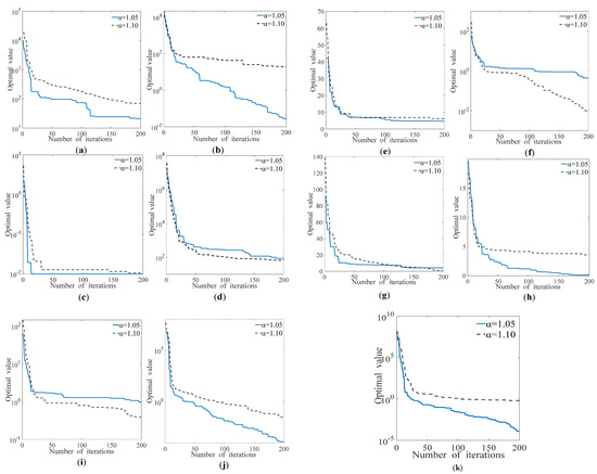
Figure 5.
Comparison of different values in the HDBBO algorithm (a–k) on the convergence of − .(a) convergence of different on benchmark function ; (b) convergence of different on benchmark function ; (c) convergence of different on benchmark function ; (d) convergence of different on benchmark function ; (e) convergence of different on benchmark function ; (f) convergence of different on benchmark function ; (g) convergence of different on benchmark function ; (h) convergence of different on benchmark function ; (i) convergence of different on benchmark function ; (j) convergence of different on benchmark function ; (k) convergence of different on benchmark function .
The solid and dotted lines in Figure 5 represent the convergence curves of the functions when and , respectively. When , the simulation results of the , , and were more accurate than when in the improved BBO algorithm. Nevertheless, the improved BBO algorithm demonstrated superior convergence curves for the other eight benchmark functions when the value of was . Indeed, the optimal value could be quickly received by the HDBBO algorithm with an increase in the number of iterations.
In general, the HDBBO algorithm was superior to the other two algorithms in terms of optimization accuracy, iterative speed, and distribution of the Pareto optimal solution, which implied that it has an excellent data development ability while avoiding local optimization because of these improved strategies. Furthermore, through a set of comparative experiments, we confirmed that is more appropriate for the hyperbolic tangent mobility model in the improved BBO algorithm.
4. Conclusions
Aiming to overcome the challenges of the BBO algorithm such as slow convergence speed and insufficient search ability, we designed an improved BBO algorithm containing three novel strategies. Specifically, after replacing the mobility model of the BBO algorithm, the migration operation and mutation operation were improved and adjusted. The introduction of a nonlinear hyperbolic tangent migration model and micro-disturbance factor is beneficial to both global and local optimization. At the same time, the dual-mode mutation operation of Gaussian mutation and BBO mutation is beneficial to preserve the high-quality solution vector after mutation. Moreover, it promotes the accurate search of the solution vector in the local scope, so as to reduce the influence of the inferior solution vector on the whole solution set. Furthermore, through the combination of theoretical analysis and simulation experiments, we found that the HDBBO algorithm has clear advantages over the BBO and GBBO algorithms. The HDBBO algorithm can effectively avoid the problem of local optimization and possesses a strong data development ability, which will be more beneficial for the optimization problems of multi-objective or nonlinear complex functions in future work. In addition, the optimal scheduling of microgrids at present is usually constrained by a variety of conditions and more consideration needs to be given to multi-objective optimal scheduling. Thus, we are also committed to applying the HDBBO algorithm to the multi-objective optimization of microgrids.
Author Contributions
Conceptualization, Q.Z. and B.Y.; methodology, B.Y.; software, Q.Z.; validation, Q.Z., L.W., and B.Y.; formal analysis, Q.Z. and B.Y.; investigation, B.Y.; resources, L.W.; data curation, Q.Z.; writing—original draft preparation, Q.Z.; writing—review and editing, L.W.; visualization, B.Y.; supervision, L.W.; project administration, L.W.; funding acquisition, L.W. All authors have read and agreed to the published version of the manuscript.
Funding
This work was supported by the Natural Science Research Program of the Colleges and Universities of Anhui Province under grant KJ2020ZD39, the Open Research Fund of Anhui Key Laboratory of Detection Technology and Energy Saving Devices under grant DTESD2020A02, the Scientific Research Project of the "333 project" in Jiangsu Province under grant BRA2018218, the Postdoctoral Research Foundation of Jiangsu Province under grant 2020Z389, and the Qing Lan Project of colleges and universities in Jiangsu province.
Data Availability Statement
Not applicable.
Conflicts of Interest
The authors declare no conflict of interest.
References
- Zhang, J.H.; Li, A.P.; Liu, X.M. Hybrid genetic algorithm for a type-II robust mixed-model assembly line balancing problem with interval task times. Adv. Manuf. 2019, 7, 117–132. [Google Scholar] [CrossRef]
- Chaudhari, R.; Vora, J.J.; Prabu, S.S.; Palani, I.A.; Patel, V.K.; Parikh, D.M. Pareto optimization of WEDM process parameters for machining a NiTi shape memory alloy using a combined approach of RSM and heat transfer search algorithm. Adv. Manuf. 2021, 9, 64–80. [Google Scholar] [CrossRef]
- Cui, L.; Tao, Y.; Deng, J.; Liu, X.; Xu, D.; Tang, G. BBO-BPNN and AMPSO-BPNN for multiple-criteria inventory classification. Expert Syst. Appl. 2021, 175, 114842. [Google Scholar] [CrossRef]
- Lim, W.L.; Wibowo, A.; Desa, M.I.; Haron, H. A Biogeography-Based Optimization Algorithm Hybridized with Tabu Search for the Quadratic Assignment Problem. Comput. Intell. Neurosci. 2016, 2016, 5803893. [Google Scholar] [CrossRef] [PubMed]
- Kalpanadevi, M.; Neela, R. BBO Algorithm for Line Flow Based WLS State Estimation. Mater. Today Proc. 2018, 5, 318–328. [Google Scholar] [CrossRef]
- Simon, D. Biogeography-Based Optimization. IEEE Trans. Evol. Comput. 2008, 12, 702–713. [Google Scholar] [CrossRef]
- Ma, H.P.; Li, X.; Lin, S.D. Analysis of migration rate models for biogeography-based optimization. J. Southeast Univ. 2009, 39, 16–21. [Google Scholar]
- Giri, P.K.; De, S.S.; Dehuri, S. Adaptive neighbourhood for locally and globally tune biogeography based optimization algorithm. J. King Saud Univ.-Comput. Inf. Sci. 2021, 33, 453–467. [Google Scholar]
- Jalaee, S.A.; Shakibaei, A.; Horry, H.R.; Akbarifard, H.; GhasemiNejad, A.; Robati, F.N.; Zarin, N.A. A new hybrid metaheuristic method based on biogeography-based optimization and particle swarm optimization algorithm to estimate money demand in Iran. MethodsX 2021, 8, 101226. [Google Scholar] [CrossRef]
- Zhang, X.; Kang, Q.; Cheng, J.; Wang, X. A novel hybrid algorithm based on Biogeography-Based Optimization and Grey Wolf Optimizer. Appl. Soft Comput. 2018, 67, 197–214. [Google Scholar] [CrossRef]
- Zhao, F.; Qin, S.; Zhang, Y.; Ma, W.; Zhang, C.; Song, H. A two-stage differential biogeography-based optimization algorithm and its performance analysis. Expert Syst. Appl. 2019, 115, 329–345. [Google Scholar] [CrossRef]
- Singh, S.K.; Sinha, N.; Goswami, A.K.; Sinha, N. Powersystem harmonic estimation using biogeography hybridized recursive least square algorithm. Int. J. Electr. Power Energy Syst. 2016, 83, 219–228. [Google Scholar] [CrossRef]
- Chen, Y.; He, F.; Li, H.; Zhang, D.; Wu, Y. A full migra-tion BBO algorithm with enhanced population qualitybounds for multimodal biomedical image registration. Appl. Soft Comput. 2020, 93, 106335. [Google Scholar] [CrossRef]
- Zhang, S.; Xu, S.; Zhang, W.; Yu, D.; Chen, K. A hybrid a-pproach combining an extended BBO algorithm with an intuitionistic fuzzy entropy weight method for QoS-aware manufacturing service supply chain optimization. Neurocomputing 2018, 272, 439–452. [Google Scholar] [CrossRef]
- Hadidi, A. A robust approach for optimal design of plate fin heat exchangers using biogeography based optimization (BBO) algorithm. Appl. Energy 2015, 150, 196–210. [Google Scholar] [CrossRef]
- Liu, F.; Gu, B.; Qin, S.; Zhang, K.; Cui, L.; Xie, G. Power grid partition with improved biogeography-based optimization algorithm. Sustain. Energy Technol. Assess. 2021, 46, 101267. [Google Scholar] [CrossRef]
- Zhang, Y.; Gu, X. Biogeography-based optimization algorithm for large-scale multistage batch plant scheduling. Expert Syst. Appl. 2020, 162, 113776. [Google Scholar] [CrossRef]
- Zheng, Y.J.; Ling, H.F.; Shi, H.H.; Chen, H.S.; Chen, S.Y. Emergency railway wagon scheduling by hybrid biogeography-based optimization. Comput. Oper. Res. 2014, 43, 1–8. [Google Scholar] [CrossRef]
- Giri, P.K.; De, S.S.; Dehuri, S. A Novel Locally and Globally Tuned Biogeography-based Optimization Algorithm. Soft. Comput. Theor. Appl. 2018, 583, 635–647. [Google Scholar]
- Wang, Y.; Zhang, Z.; Yan, Z.; Jin, Y. Biogeography-based optimization algorithms based on improved migration rate models. J. Comput. Appl. 2019, 39, 2511–2516. [Google Scholar]
- Zhang, X.; Wang, D.; Fu, Z.; Liu, S.; Mao, W.; Liu, G.; Jiang, Y.; Li, S. Novel biogeography-based optimization algorithm with hybridmigration and global-best Gaussian mutation. Appl. Math. Model. 2020, 86, 74–91. [Google Scholar] [CrossRef]
- Chen, X. Novel dual-population adaptive differential evolution algorithm for large-scale multi-fuel economic dispatch with valve-point effects. Energy 2020, 203, 117874. [Google Scholar] [CrossRef]
- Zhang, X.; Kang, Q.; Tu, Q.; Cheng, J.; Wang, X. Efficient and merged biogeography-based optimization algorithm for global optimization problems. Soft. Comput. 2019, 23, 4483–4502. [Google Scholar] [CrossRef]
- Nemade, S.N.; Kolte, M.T.; Nemade, S. Multi-user Detection in DS-CDMA System Using Biogeography Based Optimization. Proc. Comput. Sci. 2015, 49, 289–297. [Google Scholar] [CrossRef][Green Version]
- Wang, N.; Wei, L.S. A Novel Biogeography-Based Optimization Algorithm Research Based on GA. J. Syst. Simul. 2020, 32, 1717–1723. [Google Scholar]
Publisher’s Note: MDPI stays neutral with regard to jurisdictional claims in published maps and institutional affiliations. |
© 2022 by the authors. Licensee MDPI, Basel, Switzerland. This article is an open access article distributed under the terms and conditions of the Creative Commons Attribution (CC BY) license (https://creativecommons.org/licenses/by/4.0/).