Article

Long-Term Bifurcation and Stochastic Optimal Control of a Triple-Delayed Ebola Virus Model with Vaccination and Quarantine Strategies

1
Department of Mathematics, Sun Yat-sen University, Guangzhou 510275, China
2
School of Computer Science and Cyber Engineering, Guangzhou University, Guangzhou 510006, China
3
LPAIS Laboratory, Faculty of Sciences Dhar El Mahraz, Sidi Mohamed Ben Abdellah University, Fez 30000, Morocco
*
Authors to whom correspondence should be addressed.
Fractal Fract. 2022, 6(10), 578; https://doi.org/10.3390/fractalfract6100578
Submission received: 9 September 2022 / Revised: 30 September 2022 / Accepted: 3 October 2022 / Published: 10 October 2022

Abstract

:
Despite its high mortality rate of approximately 90 % , the Ebola virus disease (EVD) has not received enough attention in terms of in-depth research. This illness has been responsible for over 40 years of epidemics throughout Central Africa. However, during 2014–2015, the Ebola-driven epidemic in West Africa became, and remains, the deadliest to date. Thus, Ebola has been declared one of the major public health issues. This paper aims at exploring the effects of external fluctuations on the prevalence of the Ebola virus. We begin by proposing a sophisticated biological system that takes into account vaccination and quarantine strategies as well as the effect of time lags. Due to some external perturbations, we extend our model to the probabilistic formulation with white noises. The perturbed model takes the form of a system of stochastic differential equations. Based on some non-standard analytical techniques, we demonstrate two main approach properties: intensity and elimination of Ebola virus. To better understand the impact of applied strategies, we deal with the stochastic control optimization approach by using some advanced theories. All of this theoretical arsenal has been numerically confirmed by employing some real statistical data of Ebola virus. Finally, we mention that this work could be a rich basis for further investigations aimed at understanding the complexity of Ebola virus propagation at pathophysiological and mathematics levels.
MSC:
65M06; 39A14; 35L53; 92D25

1. Introduction

In 2013, EVD was declared an epidemic. Guinea, Liberia and Sierra Leone were the most affected regions of 2013–2016, where the virus caused huge losses and disrupted the socioeconomic balance [1]. On 8 August 2014, WHO declared the EVD pandemic in West Africa a Public Health Emergency of International Concern (PHEIC), which is designated only for events with a risk of potential international spread or that require a coordinated international response. Over the duration of the epidemic, EVD spread to seven more countries: Italy, Mali, Nigeria, Senegal, Spain, the United Kingdom and the United States [2,3]. Ebola viruses belong to the Filoviridae family like Marburg and Lloviu viruses [4,5]. Currently, five species of Ebola virus have been described: Zaire, Reston, Bundibugyo, Sudan and Taï Forest [6,7,8]. They are highly pathogenic viruses, classified as level 4. They are responsible, for the most part, for viral hemorrhagic fevers (VHF) most often fatal in human and non-human primates, during transmission by contact with biological fluids [9,10]. This virus, known since 1976, had already caused several episodes in Africa but none of such rapid evolution and such serious impact on public health [11]. Indeed, before the year 2014, there were 1580 deaths with all epidemics combined. The month of December 2013 was the starting point for the transmission of the virus: the first case was detected in Guinea [12]. After that, the virus infected a number of countries in the world (see Figure 1). The cases observed outside Africa have been few and linked to travel or the repatriation of caregivers [13]. Before this epidemic, West Africa did not know the Ebola virus, which had been isolated in Central Africa [14]. In addition to this lack of knowledge, there are social, economic and cultural factors that have favored the spread: the mobility of populations, funeral rites, the reluctance to follow government recommendations and in particular the distrust of foreign caregivers [15]. Furthermore, the epidemic has worsened a previously unfavorable economic situation in the affected African countries [16].
On 8 August 2014, faced with the scale of the epidemic, the Director General of the WHO (World Health Organization) formally announced that this surge of the Ebola virus is an emergency at the international level, which is related to public health [17]. An international mobilization was then formed. Means of prevention have been put in place to prevent the spread of the virus from person to person [18]. Common practices such as funeral rites have been stopped. No treatment or vaccine was known at the time [19]. Faced with the virulence of the Ebola virus and in view of the increasing number of deaths, researchers have tried to find solutions to end the epidemic. Search procedures have been accelerated. Experimental treatments and vaccines have gradually emerged [20]. The census of cases in Europe has reinforced the concern of Westerners about the epidemic. European countries, and in particular France, have prepared for the possibility of a national epidemic [21].
The foundations of epidemiology based on compartmental models were laid by physician Sir Ronald Ross who, in 1911, wrote the first compartmental model of malaria using [22]. Mathematical models can therefore help to determine the appropriate response and the effort required to control an infectious disease. More specifically, they help the scientific community to easily understand the transmission processes of infectious diseases and to evaluate the effectiveness of the different control strategies implemented to contain an epidemic [23]. Several mathematical models have been proposed to explain the dynamics of infectious diseases, some of which have included control strategies such as quarantine, isolation, contact tracing, and vaccination [24,25,26,27,28]. Berge et al. [29] suggested a deterministic model for explaining the transmission mechanism of Ebola virus that included a commonality between the epidemics and endemic phases. The model included both the direct and indirect modes of interactions within the three distinct populations: animals, humans and fruit bats. Actually, the paper [29] is considered to be an extension of the study [23], which presented a model that includes both the indirect and direct spread of Ebola virus and a source that continuously provides the Ebola virus. Further, models have been proposed that attempt to comprehend different intervention policies aimed at limiting the transmission of Ebola virus [30]. Through mathematical models, refs. [31,32,33] studied the impact of vaccines on the dynamics of the epidemics, and [34] looked at the issue of quarantining. In another work, Berge et al. [35] proposed a system of equations describing the effectiveness of the tracing of interactions as a control measure in case of Ebola virus. Researchers have recently shown a strong interest in optimal control theory of epidemic problems particularly in controlling the Ebola virus. Numerous strategies and prevention programs have been used to investigate the optimal control analysis of problems that reflects the dynamics of Ebola virus [36,37]. Particularly, Area et al. [38] introduced an Ebola virus model to explain how vaccination of the vulnerable population would affect the spread of diseases. Subsequently, they studied two different control problems for understanding the transmission mechanism of Ebola virus and its control through vaccination.
In fact, when dealing with biological systems, more realistic properties should be included such as the time delay. This property is used to describe the evolution of certain phenomena, which does not only depend on current states but also on the past [39,40,41]. Specifically, in the Ebola situation, time lag is widely employed to understand the viral interactions. In this paper, we focus on the effect of vaccination plan, quarantine strategy and time delay on the long-run behavior of Ebola virus. From mathematical modeling, the Ebola dynamics can be modeled in the general form by a system of four ordinary differential equations:
d I s = { A h I s I e ( t ) ( u + v ) I s ( t ) + v I s ( t ς 1 ) e u ς 1 + w I e ( t ς 2 ) e u ς 2 + z I q ( t ς 3 ) e u ς 3 } d t , d I e = h I s I e ( u + α 1 + q + w ) I e d t , d I q = q I e ( u + α 2 + z ) I q d t , d I r = { v I s + w I e + z I q u I r v I s ( t ς 1 ) e u ς 1 w I e ( t ς 2 ) e u ς 2 z I q ( t ς 3 ) e u ς 3 } d t ,
where I s ( t ) denotes the number of susceptible class, I e ( t ) is the number of infected people, I q ( t ) stands for the number of quarantined population and I r ( t ) describes the size of recovered class. The parameter A is the constant recruitment into I s class; h is the rate at which the Ebola virus is spreading in the population; v is the vaccination rate of the susceptible individuals and u represents the natural death rate, which is constant for all compartments. The parameter w denotes the recovery rate of individuals that remain infectious for a period of 1 / w ; the notations α 1 and α 2 are the respective disease-related death rates in the infected and quarantined populations. The rate at which the infected population becomes quarantined is denoted by q, whereas z is the rate at which the quarantine population is achieving recovery. For biological purposes, we shall assume that all of the parameters used in the model are constant and positive. In system (1), the positive quantity ς 1 stands for the length of immunity period of the vaccinated, and the term e u ς 1 represents the probability that the susceptible individuals are vaccinated at time t ς 1 and still alive at time t. The positive quantities ς 2 and ς 3 reflect, respectively, the length of immunity period of the recovered from infected and quarantined individuals. e u ς 2 and e u ς 2 denote the probability that the infected and quarantined individuals have been immunized at times t ς 2 and t ς 3 , and the probability they have lost immunity but are still alive at time t.
In the complex and real world, environmental fluctuations influence the spread of infectious diseases and make it more complicated to foresee their behavior [42,43,44,45]. In such cases, deterministic systems, while able to make very informative forecasts and previsions, are not appropriate enough [46,47,48,49]. So, there is a pressing need for a developed mathematical model that can take into account the randomness effect, especially in the context of a harmful infectious disease such as the Ebola virus. In this context, many scholars have suggested and evolved a large number of stochastic models that describe the Ebola virus propagation dynamics from different angles and viewpoints [50]. In this research, we will use the proportional white noise approach to better reflect the reality of Ebola spreading. In an uncertain and constantly changing environment, the dynamic system can be disturbed by the white noises. As a result, the following system of SDEs (being a counterpart of model (1)) may be presented:
d I s = { A h I s I e ( t ) ( u + v ) I s ( t ) + v I s ( t ς 1 ) e u ς 1 + w I e ( t ς 2 ) e u ς 2 + z I q ( t ς 3 ) e u ς 3 } d t + ϖ s I s ( t ) d P s ( t ) , d I e = h I s I e ( u + α 1 + q + w ) I e d t + ϖ e I e ( t ) d P e ( t ) , d I q = q I e ( u + α 2 + z ) I q + P q ( t ) d t + ϖ q I q ( t ) d P q ( t ) , d I r = { v I s + w I e + z I q u I r v I s ( t ς 1 ) e u ς 1 w I e ( t ς 2 ) e u ς 2 z I q ( t ς 3 ) e u ς 3 } d t + ϖ r I r ( t ) d P r ( t ) ,
where ϖ s , ϖ e , ϖ q and ϖ r are the positive linear intensities associated, respectively, to the mutually independent Brownian motions P s ( t ) , P e ( t ) , P q ( t ) and P r ( t ) . These latter, and all the random variables that will be met in this paper, are defined on a filtered probability space ( Ω , E , { E t } t 0 , P Ω ) endowed with a filtration { E t } t 0 that verifies the usual hypotheses [51]. By employing the identical techniques presented in (ref. [46], Theorem 2), we can facilely demonstrate that for every positive started value, there is a single positive solution to the probabilistic system (2). This indicates that the model (2) is well-constructed scientifically.
Analogous to the non-probabilistic framework, the primary goal of examining the dynamics of the probabilistic epidemic systems is to establish the conditions that ensure disappearance and continuation of illness [43,52,53,54,55]. In this research, we try to cope with the disappearance of the Ebola virus and the existence of a single stationary distribution of system (2). Of course, ergodic steady distribution implies the permanence of the Ebola infection. Technically, one of the usual methods to ensure ergodicity is the Lyapunov candidate function, which gives just sufficient conditions in the majority of cases [56,57,58]. Therefore, the first problematic of this research can be formulated as follows: is it feasible to supply the acute threshold (sufficient and necessary condition) for the stationarity of the system Ebola and the disappearance of the Ebola virus? Specifically, the present study suggests a novel method for dealing with biological systems perturbed by white noises. We offer the sufficient and almost required criterion for the ergodic property of our model and the disappearance of Ebola virus. Using a probabilistic auxiliary equation, we found the acute threshold S . In other words, if S > 1 , then model (2) has a single steady ergodic distribution, and if S < 1 , then the density of infected class will quickly converge to zero.
On the other hand, optimization theory of dynamical systems, especially as it relates to epidemic illnesses, has received a lot of interest from researchers in recent years. Several control methods have been suggested and successfully implemented to various epidemic diseases. The primary goal of the theory of optimal control, particularly in epidemiological problems, is to present a preventive measure that restricts the spread of the disease and to portray the transmission mechanism of the infections [59,60,61]. This theory has filled many loopholes in different fields, notably those that depends on dynamic system(s), such as physics and business [62,63]. Interested readers are advised to consult [64] and the bibliography therein for the details of step-by-step optimality criteria. In general, when dealing with controlling of contagious diseases, the ideal approaches are to mitigate infectious disease to a minimum standard while spending the least amount of money on the overall control program. Regarding real life scenarios, a much lower number of articles are available in the literature, and usually the investigated data are retrieved from the laboratories and clinics. One must cite many works and make many attempts in various mathematical formulas to develop a model that suits the data points well. After developing a very basic system, it is possible to modify it by incorporating various features of the disease that may fit the clinical data as well as experimentally. Liu and Meng [65] worked on the dynamics of an optimal stochastic harvesting problem with delay and derived a few insightful results, including the maximum limit of sustainability. As Ebola virus contains both stochasticity and delay, we intend to study this disease while considering these facts in modeling, which has not been done yet to the best of our knowledge.
The remaining parts of the work are as follows. In Section 2, we treat the dynamical bifurcation of the stochastic system (2) by proving that S is the sharp threshold between stationarity and extinction of the Ebola virus. In Section 3, we deal with the Ebola system (2) under stochastic control by using the well-known methods of delayed stochastic control theory. In Section 4, we present the parameter estimation approach for Ebola virus with real statistical data of Western Guinea. In Section 5, we support our findings with some computer simulations, and we derive the main conclusions of the article in Section 6.

2. Stochastic Long-Run Dynamics of Ebola Model

This section exhibits a new approach to belay the dynamical bifurcation of our perturbed system. Since the dynamic of the recovered compartment has no influence on the infection transmission behavior, we can neglect the last equation of (2). We consider the following reduced model:
d I s = { A h I s I e ( t ) ( u + v ) I s ( t ) + v I s ( t ς 1 ) e u ς 1 + w I e ( t ς 2 ) e u ς 2 + z I q ( t ς 3 ) e u ς 3 } d t + ϖ s I s ( t ) d P s ( t ) , d I e = h I s I e ( u + α 1 + q + w ) I e d t + ϖ e I e ( t ) d P e ( t ) , d I q = q I e ( u + α 2 + z ) I q + P q ( t ) d t + ϖ q I q ( t ) d P q ( t ) ,
with initial historical data I s ( t ) , I e ( t ) , I q ( t ) L 1 [ ς , 0 ] ; R + 3 , where ς = max { ς 1 , ς 2 , ς 3 } .
To probe the long-run dynamics of our proposed Ebola model (3), we will use an additional perturbed equation associated with the differential equation of the total class T ( t ) = I s ( t ) + I e ( t ) + I q ( t ) + I r ( t ) . This new equation illustrates the biological situation when Ebola does not exist I e ( t ) = 0 . Let J ( t ) be a Markov process that verifies the following probabilistic formulation:
d J ( t ) = A ( u + v ) J ( t ) + v J ( t ς 1 ) e u ς 1 d t + d Σ s ( t ) , J ( 0 ) = T ( 0 ) ,
where the probabilistic part is given by
d Σ s ( t ) = ϖ s I s ( t ) d P s ( t ) + ϖ e I e ( t ) d P e ( t ) + ϖ q I q ( t ) d P q ( t ) + ϖ r I r ( t ) d P r ( t ) ,
and T ( 0 ) = I s ( 0 ) + I e ( 0 ) + I q ( 0 ) + I r ( 0 ) . From Lemma 2.11 of [66], we infer that Equation (4) is scientifically well-posed and the time average of its unique solution is estimated as follows:
lim t t 1 0 t J ( s ) d s = A u + v ( 1 e u ς 1 ) a.s.
In line with the probabilistic comparison result [67], we show that T ( t ) J ( t ) a.s. So, asymptotically, we can use inequality (5) to obtain information about the mean long-time behavior of T ( t ) . Concerning the latter, we also present the following result.
 Lemma 1.
Let I s , I e , I q , I r be the unique positive solution of (2). Then, for any φ 0.5 , 0.5 + u m , where m = max { ϖ s 2 , ϖ e 2 , ϖ q 2 , ϖ r 2 } , we have the following estimate:
lim sup t 1 t 0 t E { Ω , P } T 2 φ ( s ) d s 2 χ Ξ ,
where χ = sup T > 0 A T 2 φ 1 0.5 Ξ T 2 φ and Ξ = u 0.5 ( 2 φ 1 ) m .
For a detailed demonstration of the above lemma, we refer the reader to the proof of Lemma 2.2 in [66].
Before stating the main theorem of this section, we present in Table 1 some notations used later and define the following quantity:
S = 1 ( u + α 1 + q + w ) h A u + v ( 1 e u ς 1 ) 0.5 ϖ e 2 .
To exhibit possible future scenarios for the spread of Ebola, we offer the next principal result.
 Theorem 1.
The Ebola propagation process described by system (3) has two possible scenarios:
1. 
The stationary case ( S > 1 )—that is, ecosystem (3)—admits a single ergodic limiting distribution π E ( · ) . In other words, Ebola epidemic persists.
2. 
The eradication case ( S < 1 )—that is, the Ebola epidemic—will disappear with full probability.
Proof. 
First case: when S > 1 ̲ . We apply Itô’s rule to the function ln I e ( t ) , then
d ln I e ( t ) = h I s ( t ) ( u + α 1 + q + w ) 0.5 ϖ e 2 d t + ϖ e d P e ( t ) .
Once again, Itô’s rule leads to
d J ( t ) I s ( t ) + v e u ς 1 t ς 1 t J ( s ) d s v e u ς 1 t ς 1 t I s ( s ) d s = { A u + v 1 e u ς 1 J ( t ) A + h I s ( t ) I e ( t ) + u + v 1 e u ς 1 I s ( t ) w I e ( t ς 2 ) e u ς 2 z I q ( t ς 3 ) e u ς 3 } d t + ϖ e I e ( t ) d P e ( t ) + ϖ q I q ( t ) d P q ( t ) + ϖ r I r ( t ) d P r ( t ) .
Now, we merge the above two equations as follows:
d ln I e ( t ) h u + v 1 e u ς 1 J ( t ) I s ( t ) + v e u ς 1 t ς 1 t J ( s ) d s v e u ς 1 t ς 1 t I s ( s ) d s = { h I s ( t ) ( u + α 1 + q + w ) 0.5 ϖ e 2 + h J ( t ) h 2 u + v 1 e u ς 1 I s ( t ) I e ( t ) h I s ( t ) + h w u + v 1 e u ς 1 I e ( t ς 2 ) e u ς 2 + h z u + v 1 e u ς 1 I q ( t ς 3 ) e u ς 3 } d t + ϖ e d P e ( t ) h ϖ e u + v 1 e u ς 1 I e ( t ) d P e ( t ) h ϖ q u + v 1 e u ς 1 I q ( t ) d P q ( t ) h ϖ r u + v 1 e u ς 1 I r ( t ) d P r ( t ) .
In line with the positivity of the solution, we obtain
d ln I e ( t ) h u + v 1 e u ς 1 J ( t ) I s ( t ) + v e u ς 1 t ς 1 t J ( s ) d s v e u ς 1 t ς 1 t I s ( s ) d s h J ( t ) ( u + α 1 + q + w ) 0.5 ϖ e 2 h 2 u + v 1 e u ς 1 I s ( t ) I e ( t ) d t + ϖ e d P e ( t ) h ϖ e u + v 1 e u ς 1 I e ( t ) d P e ( t ) h ϖ q u + v 1 e u ς 1 I q ( t ) d P q ( t )
h ϖ r u + v 1 e u ς 1 I r ( t ) d P r ( t ) .
For simplicity of notation, we set
O ( t ) = ln I e ( t ) h u + v 1 e u ς 1 { J ( t ) I s ( t ) + v e u ς 1 t ς 1 t J ( s ) d s v e u ς 1 t ς 1 t I s ( s ) d s } .
An integration from 0 to t on both sides of (8) gives
O ( t ) O ( 0 ) 0 t h J ( s ) d s ( u + α 1 + q + w ) t 0.5 ϖ e 2 t h 2 u + v 1 e u ς 1 0 t I s ( s ) I e ( s ) d s h ϖ e u + v 1 e u ς 1 0 t I e ( s ) d P e ( s ) h ϖ q u + v 1 e u ς 1 0 t I q ( s ) d P q ( s ) h ϖ r u + v 1 e u ς 1 0 t I r ( s ) d P r ( s ) + ϖ e P e ( t ) .
Thus, we obtain
0 t h I s ( s ) I e ( s ) d s u + v 1 e u ς 1 h 0 t h J ( s ) d s u + v 1 e u ς 1 h ( u + α 1 + q + w ) + 0.5 ϖ e 2 t ϖ e 0 t I e ( s ) d P e ( s ) ϖ q 0 t I q ( s ) d P q ( s ) ϖ r 0 t I r ( s ) d P r ( s ) h O ( t ) u + v 1 e u ς 1 + h O ( 0 ) u + v 1 e u ς 1 + ϖ e P e ( t ) .
By employing the strong law of large numbers for martingale [51] and (5), we have
lim inf t 1 t 0 t h I s ( s ) I e ( s ) d s u + v 1 e u ς 1 h { lim inf t 1 t 0 t h J ( s ) d s
( u + α 1 + q + w ) + 0.5 ϖ e 2 } = 1 h u + v 1 e u ς 1 ( u + α 1 + q + w ) S 1 .
By using the definitions of the subsets W a , W b and W c appearing in Table 1, we easily obtain
lim inf t 1 t 0 t E { Ω , P } h I s ( s ) I e ( s ) 1 W a d s lim sup t 1 t 0 t E { Ω , P } h I s ( s ) I e ( s ) 1 W b d s lim sup t 1 t 0 t E { Ω , P } h I s ( s ) I e ( s ) 1 W c d s + lim inf t 1 t 0 t E { Ω , P } h I s ( s ) I e ( s ) d s ,
where E { Ω , P } denotes the mathematical expectation. In accordance with (10), we have
lim inf t 1 t 0 t E { Ω , P } h I s ( s ) I e ( s ) 1 W a d s h Υ lim sup t 1 t 0 t E { Ω , P } I s ( s ) d s h Υ lim sup t 1 t 0 t E { Ω , P } I e ( s ) d s + 1 h u + v 1 e u ς 1 ( u + α 1 + q + w ) S 1 .
Consequently,
lim inf t 1 t 0 t E { Ω , P } h I s ( s ) I e ( s ) 1 W a d s 2 h Υ A u + 1 h u + v 1 e u ς 1
× ( u + α 1 + q + w ) S 1 .
We choose
Υ 0.25 u h 2 A u + v 1 e u ς 1 ( u + α 1 + q + w ) S 1 ,
then, (11) becomes
lim inf t 1 t 0 t E { Ω , P } h I s ( s ) I e ( s ) 1 W a d s 0.5 h u + v 1 e u ς 1 ( u + α 1 + q + w ) S 1 .
Let φ 0.5 , 0.5 + u m and ψ is given by ψ 1 + φ 1 = 1 . By the use of Young inequality, we obtain
lim inf t 1 t 0 t E { Ω , P } h I s ( s ) I e ( s ) 1 W a d s lim inf t t 1 0 t E { Ω , P } ( φ 1 κ h I s ( s ) I e ( s ) φ + ψ 1 κ ψ 1 W 1 d s p 1 ( ϱ b ) p lim sup t t 1 0 t E { Ω , P } T 2 φ ( s ) d s + lim inf t t 1 0 t E { Ω , P } ψ 1 κ ψ 1 W 1 d s ,
where κ is a positive constant such that
κ φ 0.125 Ξ h ( φ + 1 ) χ u + v 1 e u ς 1 ( u + α 1 + q + w ) S 1 .
According to Lemma 1, we infer that
lim inf t 1 t 0 t E { Ω , P } 1 W a d s ψ κ ψ 0.5 h u + v 1 e u ς 1 ( u + α 1 + q + w ) S 1 2 χ κ φ h φ Ξ
0.25 ψ κ ψ h u + v 1 e u ς 1 ( u + α 1 + q + w ) S 1 .
From Table 1 and Markov’s inequality, we can conclude that
W 1 W 4 ( t , ω ) d P Ω ( ω ) P Ω ( I s ( t ) x ) + P Ω ( I e ( t ) x ) x 1 E { Ω , P } I s ( t ) + I e ( t ) .
To go further, we suppose that x verifies that
x 1 0.125 ψ κ ψ u h A u + v 1 e u ς 1 ( u + α 1 + q + w ) S 1 .
Then, we obtain
lim sup t t 1 0 t E { Ω , P } 1 W d d s 0.125 ψ κ ψ h u + v 1 e u ς 1 ( u + α 1 + q + w ) S 1 .
From (12), we show that
lim inf t 1 t 0 t E { Ω , P } 1 W g d s lim sup t 1 t 0 t E { Ω , P } 1 S d d s + lim inf t 1 t 0 t E { Ω , P } 1 S a d s 0.125 ψ κ ψ h u + v 1 e u ς 1 ( u + α 1 + q + w ) S 1 .
Consequently,
lim inf t 1 t 0 t P Ω I 0 ; s , W g d s 0.125 ψ κ ψ h u + v 1 e u ς 1 ( u + α 1 + q + w ) S 1 > 0 .
Identical to the demonstration of (Lemma 3.2, ref. [68]) and the mutually limited possibilities of lemma [69], we establish the existence, uniqueness and ergodicity of a single invariant distribution for the perturbed model (3).
Second case: when S < 1 ̲ . From (6), we obtain
lim sup t t 1 ln I e ( t ) I e ( 0 ) = h lim sup t t 1 0 t I s ( s ) d s ( u + α 1 + q + w ) 0.5 ϖ e 2 h lim t t 1 0 t J ( s ) d s ( u + α 1 + q + w ) 0.5 ϖ e 2 ( u + α 1 + q + w ) S 1 < 0 a . s .
So, lim t I e ( t ) = 0 a.s. Alternatively, we can say that infection, whose dynamics is governed by model (3), could be eradicated with a rate of deterioration ( u + α 1 + q + w ) S 1 (this is the minimum benchmark value). This ends the demonstration. □

3. Stochastic Optimal Control Strategies

In this section, we intend to obtain the optimal strategies for the proposed stochastic system based on comparing different preventive measures. To accomplish this, first of all in the following, we will identify the time-dependent control variables:
 A1: 
The isolation of the vulnerable population as well as of infectives is represented by the control measure u 1 . This control strategy aims to minimize the value of the transmission coefficient β .
 A2: 
The rate of quarantine of the infected population is controlled via the function u 2 . This strategy aims to reduce the number of infectives by shifting them into the quarantine class.
Taking into account the abovementioned two control variables (i.e., u 1 and u 2 ) in the stochastic system (2), the desired control problem can be written in the form of
d I s ( t ) = { A h I s ( t ) I e ( t ) ( 1 u 1 ( t ) ) ( u + v ) I s ( t ) + v I s ( t ς 1 ) e u ς 1 + w I e ( t ς 2 ) e u ς 2 + z I q ( t ς 3 ) e u ς 3 } d t + ϖ s I s ( t ) d P s ( t ) , d I e ( t ) = h I s ( t ) I e ( t ) ( 1 u 1 ( t ) ) ( u + α 1 + q + w + u 2 ( t ) ) I e ( t ) d t + ϖ e I e ( t ) d P e ( t ) , d I q ( t ) = q I e ( t ) ( u + α 2 + z + u 2 ( t ) ) I q ( t ) d t + ϖ q I q ( t ) d P q ( t ) , d I r ( t ) = { v I s ( t ) + ( w + u 2 ( t ) ) I e ( t ) + ( z + u 2 ( t ) ) I q ( t ) u I r ( t ) v I s ( t ς 1 ) e u ς 1 w I e ( t ς 2 ) e u ς 2 z I q ( t ς 3 ) e u ς 3 } d t + ϖ r I r ( t ) d P r ( t ) ,
along with the subsidiary conditions
I s ( 0 ) > 0 , I e ( 0 ) > 0 , I q ( 0 ) > 0 , I r ( 0 ) > 0 , t [ ς , 0 ] .
Let us proceed by introducing the vectors listed below
Θ ( t ) = I s ( t ) , I e ( t ) , I q ( t ) , I r ( t ) , u ( t ) = u 1 ( t ) , u 2 ( t ) , P ( t ) = P s ( t ) , P e ( t ) , P q ( t ) , P r ( t ) ,
and
d Θ ( t ) = ψ Θ ( t ) , u ( t ) d t + ϕ Θ ( t ) d P ( t ) .
The vectors, which consist of the data at t = 0 , are as follows:
Θ 0 = I s ( 0 ) , I e ( 0 ) , I q ( 0 ) , I r ( 0 ) .
Here, ψ and ϕ are vectors that comprise the following components:
ψ 1 ( Θ ( t ) , u ( t ) ) = A h I s ( t ) I e ( t ) ( 1 u 1 ( t ) ) ( u + v ) I s ( t ) + v I s ( t ς 1 ) e u ς 1 + w I e ( t ς 2 ) e u ς 2 + z I q ( t ς 3 ) e u ς 3 , ψ 2 ( Θ ( t ) , u ( t ) ) = h I s ( t ) I e ( t ) ( 1 u 1 ( t ) ) ( u + α 1 + q + w + u 2 ( t ) ) I e ( t ) , ψ 3 ( Θ ( t ) , u ( t ) ) = q I e ( t ) ( u + α 2 + z + u 2 ( t ) ) I q ( t ) , ψ 4 ( Θ ( t ) , u ( t ) ) = v I s ( t ) + ( w + u 2 ( t ) ) I e ( t ) + ( z + u 2 ( t ) ) I q ( t ) u I r ( t ) v I s ( t ς 1 ) e u ς 1 w I e ( t ς 2 ) e u ς 2 z I q ( t ς 3 ) e u ς 3 ,
and
ϕ 1 = ϖ s I s ( t ) , ϕ 2 = ϖ e I e ( t ) , ϕ 3 = ϖ q I q ( t ) , ϕ 4 = ϖ r I r ( t ) .
The desired strategy, given the control problem (14), is to minimize the cost (objective) function defined by
G ( u ) = 0.5 E { Ω , P } { 0 T A 1 I s ( s ) + A 2 I e ( s ) + A 3 I q ( s ) + B 1 2 u 1 2 ( s ) + B 2 2 u 2 2 ( s ) d s
+ K 1 2 I s 2 ( t ) + K 2 2 I e 2 ( t ) + K 3 2 I q 2 ( t ) + K 4 2 I r 2 ( t ) } ,
here, A l , B m , K n are positive constants for l = 1 , 2 , 3 ; m = 1 , 2 ; and n = 1 , , 4 .
Physically, the foremost three integrand’ terms stand for the decreasing size of vulnerable, latent and infectious individuals; whereas, the related constants A 1 , A 2 and A 3 are used to balance the size of the underlying populations I s ( t ) , I e ( t ) and I q ( t ) , respectively. As usual, we assumed the quadratic terms 0.5 B i u 2 , = 1 , 2 in the cost functional for the preventive measures. To balance the control parameters, we utilized the B in the cost functional.
To conclude the above-stated discussion, our aim in the current research is to find the minimum value of the objective functional (19) by employing the strategies of reducing the number of vulnerable, latent and Ebola-infected people; maximizing the size of quarantine compartment; and doing all this while utilizing the least resources. In other words, the control vector u 1 ( t ) , u 2 ( t ) U aims to decrease the interactions of the vulnerable and infected people and quarantining a portion of the latent and EVD-infected people in a unit time. Thus, we are searching for control variables, which has the property
J u J ( u ) , u U ,
where U is the feasible set of controls, which is defined by
U = u i ( t ) : u i ( t ) 0 , u , max , u L 2 0 , T t 0 , T , = 1 , 2 ,
here, the notions u , max for = 1 , 2 are constant and positive. To use the well-known stochastic version of maximum principle, first of all, it is necessary to express the Hamiltonian H m ( x , u , y , z ) as
H ( Θ , u , y , z ) = ψ Θ , u , y L Θ , u + ϕ ( Θ ) , z ,
where · , · represent the usual Euclidean inner-product while y = y 1 , y 2 , y 3 , y 4 and z = z 1 , z 2 , z 3 , z 4 vectors’ components denote the associated adjoint variables. We may reproduce the stochastic minimum/maximum principle in the following form
d Θ ( t ) = H Θ , u , y , z ( t + τ ) y d t + g Θ ( t ) d P ( t ) ,
d y ( t ) = H Θ , u , y , z ( t + τ ) Θ d t + z ( t ) d P ( t ) ,
H m Θ , u , y , z = max u U H m Θ , u , y , z ,
where θ ( t ) describes the optimal trajectory of the state variable. The terminal and initial condition related to Equations (23) and (24) are
Θ ( 0 ) = x 0 ,
y T = h Θ T ( t + τ ) Θ ,
respectively. Since Equation (25) indicates that control u ( t ) (optimal) is a function of y ( t ) , z ( t ) and x ( t ) , we can write
u ( t ) = Φ Θ , y , z ,
where Φ can be obtained from Equation (25). Hence, Equations (23) and (24) may be written in another way as
d Θ ( t ) = H θ , u , y , z ( t + τ ) y d t + ϕ Θ ( t ) d P ( t ) ,
d y ( t ) = H Θ , u , y , z ( t + τ ) Θ d t + z ( t ) d P ( t ) .
As a result, the corresponding Hamiltonian is of the form
H = ( A 1 I s ( t ) + A 2 I e ( t ) + A 3 I q ( t ) + B 1 2 u 1 2 ( t ) + B 2 2 u 2 2 ( t ) + K 1 2 I s 2 ( t ) + K 2 2 I e 2 ( t ) + K 3 2 I q 2 ( t ) + K 4 2 I r 2 ( t ) ) + y 1 { A h I s ( t ) I e ( t ) ( 1 u 1 ( t ) ) ( u + v ) I s ( t ) + v I s ( t ς 1 ) e u ς 1 + w I e ( t ς 2 ) e u ς 2 + z I q ( t ς 3 ) e u ς 3 } + y 2 h I s ( t ) I e ( t ) ( 1 u 1 ( t ) ) ( u + α 1 + q + w + u 2 ( t ) ) I e ( t ) + y 3 q I e ( t ) ( u + α 2 + z + u 2 ( t ) ) I q ( t ) + y 4 { v I s ( t ) + ( w + u 2 ( t ) ) I e ( t ) + ( z + u 2 ( t ) ) I q ( t ) u I r ( t ) v I s ( t ς 1 ) e u ς 1 w I e ( t ς 2 ) e u ς 2 z I q ( t ς 3 ) e u ς 3 } + ϖ s I s ( t ) z 1 + ϖ e I e ( t ) z 2 + ϖ q I q ( t ) z 3 + ϖ r I r ( t ) z 4 .
According to the stochastic maximum principle,
d y ( t ) = H Θ , u , y , z ( t + ς ) Θ d t + z ( t ) d P ( t ) .
By taking the respective derivative of H with respect to I s , I e , I q and I r , we will obtain y 1 , y 2 , y 3 , and y 4 in the form of
d y 1 ( t ) d t = A 1 + ( y 1 y 2 ) h I e ( t ) ( 1 u 1 ( t ) ) + y 1 u + ( y 1 y 4 ) v χ 0 , T ς 1 ( y 1 ( t + ς 1 ) y 4 ( t + ς 1 ) ) v e u ς 1 + ϖ s z 1 , d y 2 ( t ) d t = A 2 + ( y 1 y 2 ) h I s ( t ) ( 1 u 1 ( t ) ) + y 2 ( u + α 1 + q + w + u 2 ( t ) ) χ 0 , T ς 2 ( y 1 ( t + ς 2 ) y 4 ( t + ς 2 ) ) w e u ς 2 y 4 ( w + u 2 ( t ) ) + ϖ e z 2 , d y 3 ( t ) d t = A 3 + y 3 u + α 2 + z + u 2 ( t ) χ 0 , T ς 3 ( y 1 ( t + τ 3 ) y 4 ( t + ς 3 ) ) z e u ς 3 y 4 ( u 2 ( t ) + z ) + ϖ q z 3 , d y 4 ( t ) d t = y 4 u + ϖ r z 4 ,
where the notation χ 0 , T ς ( = { 1 , 2 , 3 } ) denotes the characteristic function over 0 , T ς i . Due to the free terminal states (i.e., I s T , I e T , I q T , I r T R + 4 ), the transversality conditions in association with the auxiliary conditions, we have
I s ( 0 ) = I s ^ , I e ( 0 ) = I e ^ , I q ( 0 ) = I q ^ , I r ( 0 ) = I e ^ , y T = h Θ T ( t + ς ) Θ ,
and
h I s , I e , I q , I r = K 1 2 I s 2 + K 2 2 I e 2 + K 3 2 I q 2 + K 4 2 I r 2 ,
where y 1 T = K 1 I s , y 2 T = K 2 I e , y 3 T = K 3 I q , y 4 T = K 4 I r .
The next step is to consider the derivative of the function H with respect to u 1 , u 2 , yielding the following expressions that denote the characterization of the control measures (optimal) u 1 and u 2 as
u 1 = max 0 , min 1 , 1 B 1 ( y 2 y 1 ) h I s * ( t ) + I e ( t ) ) , u 2 = max 0 , min 1 , 1 B 2 ( y 4 y 2 ) I e + ( y 4 y 3 ) I q .
To obtain the required control schemes, we developed an optimum objective functional, which contains both the control variables as well as the underlying states of the system. The goal of this study is to minimize the value of cost functional subject to the proposed stochastic differential equation system (2) and the included time-delay. It is observed that the whole control problem relies on the objective functional; thus, care should be taken in its selection. Weights should be assigned to the factors that are more important when balancing the coefficient, especially in the case of two or more factors in the cost functional. Before applying the well-known Pontryagin’ principle [70], it is required to check the theory of existence for such control measures. To demonstrate such existence, one must demonstrate that within the feasible region, the control measures are bounded, by considering a sequence of control measures and their possible dependence on the states to demonstrate its convergence. By following [70], we may define the Hamiltonian associated to the problem in the following form
H = integrand in the objective functional + adjoint variables × RHS of the differential equations .
To obtain the optimality criterion, we will differentiate the function H with respect to the control variables at the optimum values of the controls u * . Further, by considering the derivative of the function H with respect to the states, one can easily obtain the adjoin equations and similarly the transversality conditions as given by relation (34).

4. Parameters Estimation and Curve Fitting

Parameter estimation is perhaps the most important step in any research related to epidemics. It is considered an inverse process—that is, given a set of state variables and a model, we identify the values of parameters that produce a good fit of the data with our model. This step in any research is difficult as there is no single numerical or analytical method that can be used. If a method gives a unique solution of the problem, still we need a good approximation of the initial data for computing a better estimates of the parameters. This is due to solving the minimization problem by matching the actual data with the model’s solution and for a good approximation, optimization solvers need initial data very close to the real data. There is a limited knowledge of the system, obtaining good parameter values for the type of biological system studied in this research can be difficult. Keeping in view the proximity and feasibility of the proposed problem, we will utilize the MATLAB routine lsqcurvefit and will perform the estimation of parameters as shown in Table 2. This technique is proffered over other available methods as this tool can handled very easily both small and large scale problems and a detailed explanations, the readers are advised to see [71]. To do so, in this research work, we considered the real Ebola cases reported in Western Guinea from the first forty weeks of the 2015 Ebola epidemic [18].
Let us express the proposed model (1) in the following functional differential equation:
d Y d t = ( F ( t , Y , θ ) , Y ( t 0 ) ) = Y 0 .
Here, F denotes the functional relationship between the independent variable, state variables and parameter θ . The strategy will be to find the value of θ such that it minimizes the difference between the reported data and the data predicted by the model. For n number of data points, actually, we want to minimize the following function
θ ¯ = i = 1 n ( y t i y ¯ t i ) 2 .
Thus, the complete optimization problem is given by
min θ ¯ , subject to Equation ( 37 ) .
By assuming the estimated values of the parameters, we simulated both the stochastic and deterministic models against the reported Ebola virus data from the first forty weeks of 2015 in Figure 2. By an inspection, one can see that the stochastic system explains the data with good agreement. The expression 1 12 k = 1 12 x k real x k approximate x k real 1.5685 e 01 was used to measure the average relative error of fitness, which actually describes the goodness of fit value. To further strengthen our findings, we calculated the relative error in small scale by using ( 1.5685 e 01 ) , which suggests that this fitness is very accurate compared with any other fitting tools.

5. Numerical Verification

5.1. Stochastic Long-Run Behavior of Ebola Virus Model

This subsection is devoted to the numerical confirmation of the theoretical results of this article. We seek to verify that S is the acute threshold of the model (3). Additionally, we probe the complex impact of independent white noises on the long-term behavior of Ebola virus. We mention that the parameters of the deterministic model are based on the real data provided in Table 2. For stochastic intensities, we select it theoretically in order to precisely audit the results obtained in the cases of stationarity and extinction of Ebola virus and to show that a dynamic bifurcation occurs at certain noise values. The solution of our model (3) is simulated in our case with the initial data: I s ( 0 ) = 700 , I e ( 0 ) = 100 , I q ( 0 ) = 300 and I r ( 0 ) = 20 . Henceforth, the units adopted for time and number of individuals are, respectively, one day and one thousand population.
Firstly, we choose the parameter values presented in Table 2, and also select ϖ s = 0.05 , ϖ e = 0.09 , ϖ q = 0.04 and ϖ r = 0.03 . By performing simple calculations, we obtain S = 3.8451 > 1 . From Theorem 1, we infer the existence of a steady distribution. By way of explanation, stationarity indicates the continuation of Ebola virus in the population over time, and the ergodic property established by Theorem 1 implies the persistence in the mean of the virus provided by the Ebola infection—that is, the time average of all classes of model (3) reach a strictly positive value, which can be seen in the Figure 3.
Now, we increase the noise amplitude as follows: ϖ s = 0.8 , ϖ e = 2.19 , ϖ q = 0.44 and ϖ r = 0.3 . In this case, we obtain S = 0.9422 < 1 . From Theorem 1, we deduce that Ebola infection will not be present in the population. Numerically, this is shown in Figure 4. Biologically, we can establish that a large amount of outside noise leads to the eradication of Ebola infection. This means that a long-term bifurcation occurs at the same critical noise values.
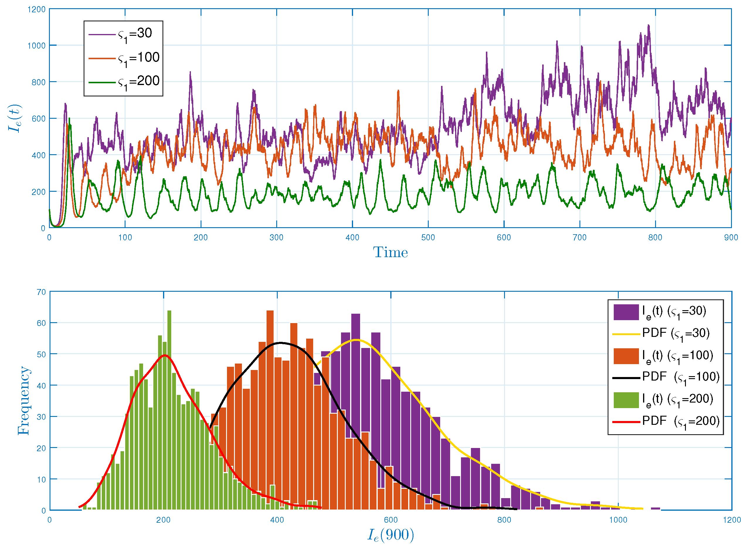
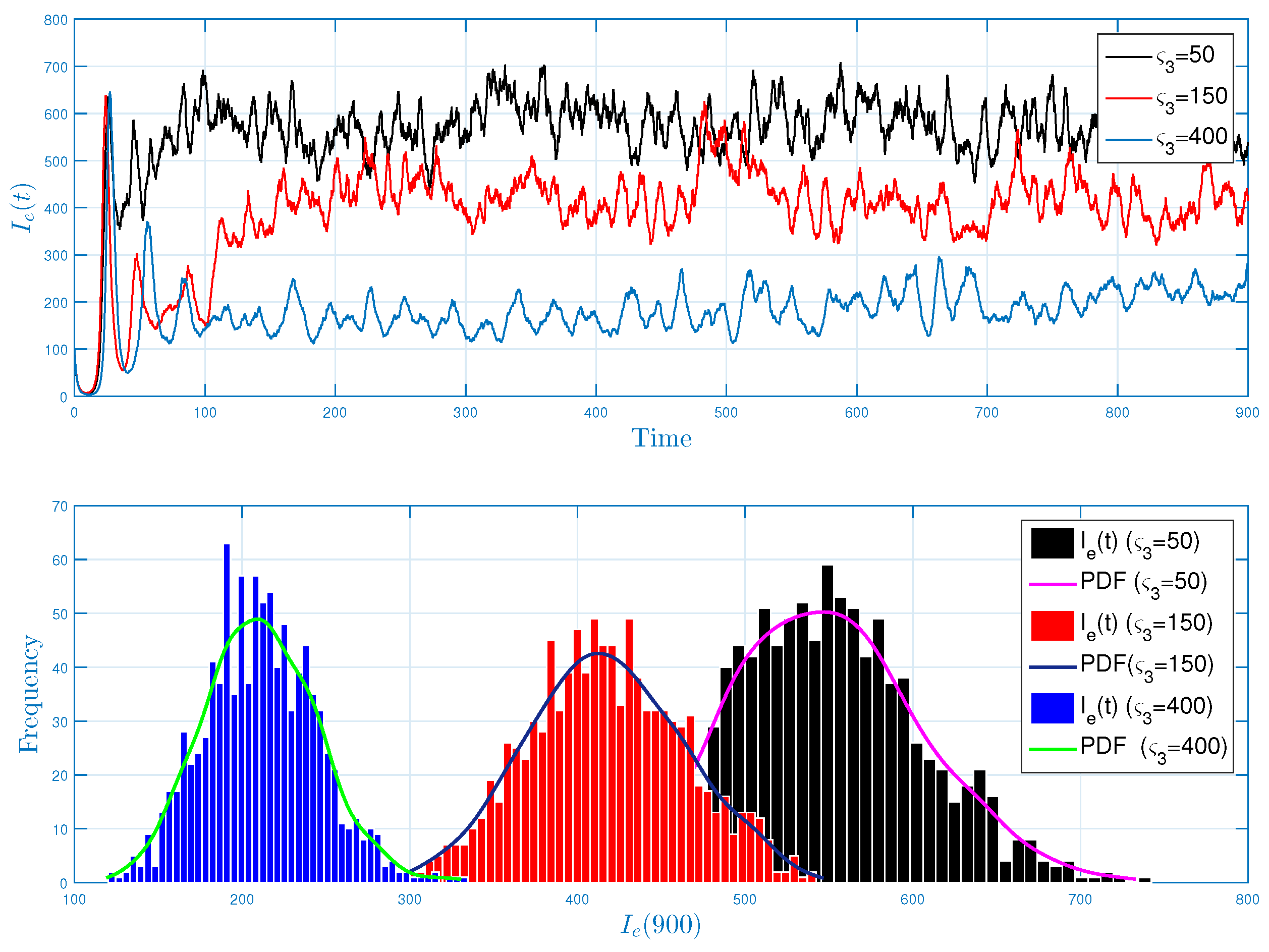
Now, we shall explore the effect of triple delays on the long-term behavior of Ebola. From Figure 5, Figure 6 and Figure 7, we show that increasing the length of the time delay leads to a significant decrease in the number of affected classes. Biologically speaking, a long delay has the greatest effect on reducing transmission. Control and tracking strategies, maximizing tracking delays—for example, using media-based technology—and increasing the effectiveness of contact tracing, have the potential to prevent contact transmissions. All this makes the control of Ebola virus possible among the population.

5.2. Stochastic Optimal Control Strategies

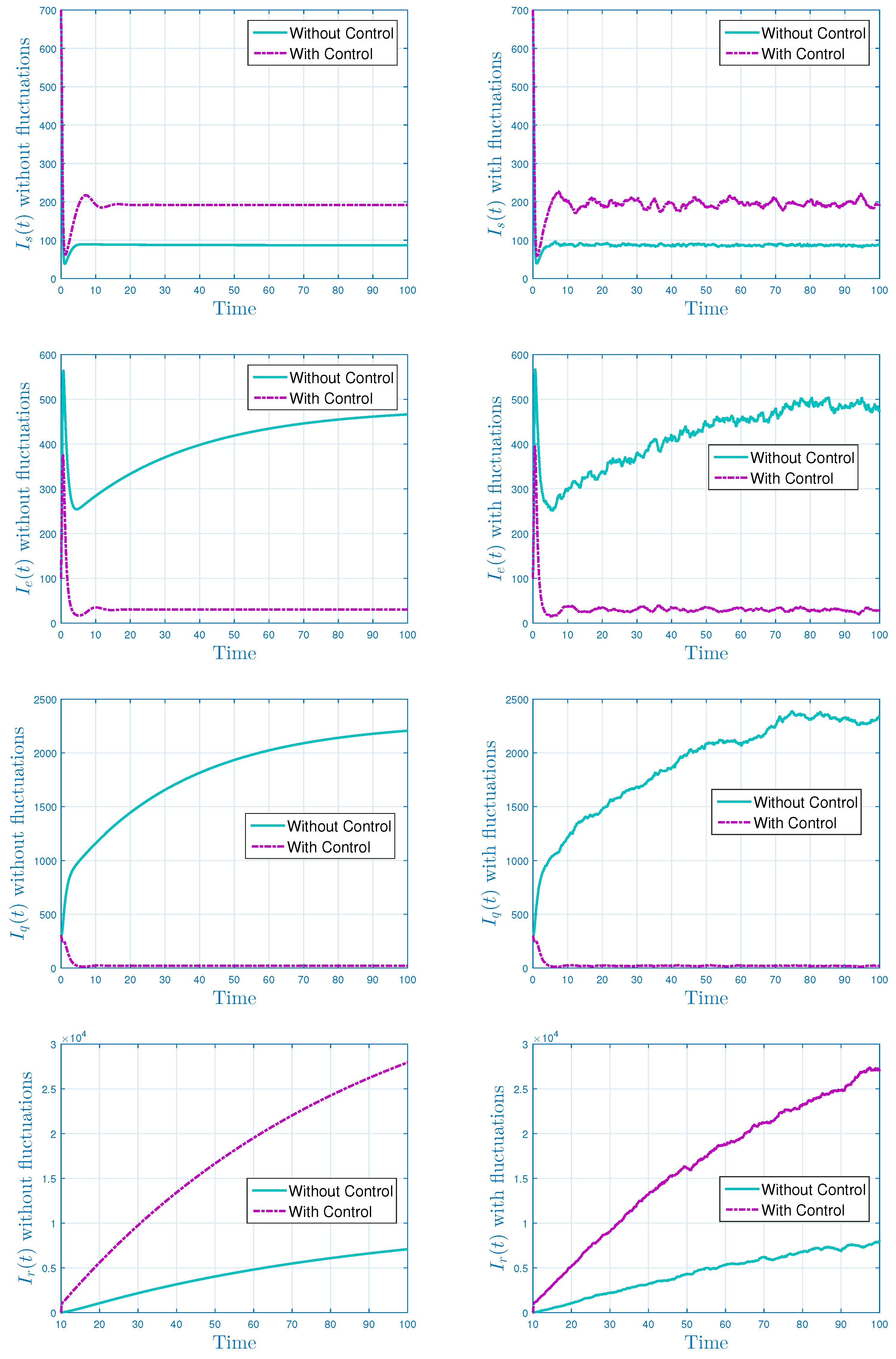
We will demonstrate the numerical (approximate) solution to the assumed stochastic control problem; we will show how the assumed control measures work by presenting the numerical example. A stochastic numerical method will be used to simulate the control system. Parallel to that, we will solve numerically the adjoint equations by using the same technique and utilizing the conditions at final time. We will code the proposed model (1) in Step 1 without using control variables; then, we will find the numerical solution of the control system. For obtaining the approximate solution of the control system, we need to simulate the adjoint system (14) with the help of a backward procedure and by considering the conditions at final time T. Since the adjoint and state variables depend upon the control parameters, the convex relationships and characterization of the control measures will be utilized in the simulation. Whereas, during the entire simulation, we assumed the parameter values from Table 2. Based on these procedures and values of the parameters, we illustrate graphical results in Figure 8, which show the usefulness of the controls in reducing the spread of Ebola.
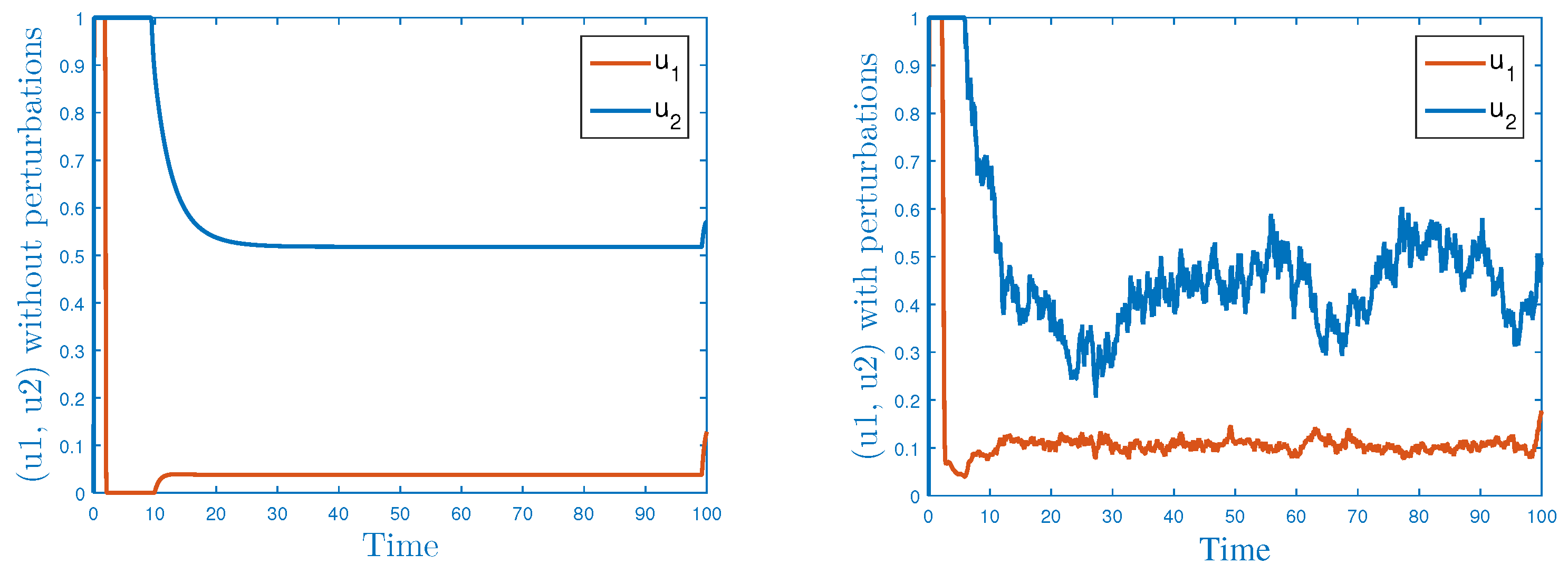
Figure 8 graphically shows the curves after and before the execution of the control strategies by employing the deterministic model (1) of the system. As the current strategy focuses on the minimization of the individuals in infected and quarantined classes, the plot shows the outcomes of the present study. Besides, we emphasized the increase in size of the recovered compartment, which is well-supported in the same figure. Further, we show that without control, the population of the quarantined class declines and will reach zero within a finite time; however, the same population tends to increase at a faster rate as we implement the control policy. Finally, Figure 9 explains the dynamics of the control variable during the entire control program both in the presence and absence of the environmental noises.

6. Conclusions

The Ebola virus has received much attention from worldwide scholars. It is caused by the Ebola virus, which takes the specific lymphocytes in the bodily immune system as the prime base and destroys its mechanism. This epidemic has a short incubation period with a high fatality rate for patients, and its treatment increases the predicted time for its transmission. This treatment strategy guarantees a more reasonable probability of affecting others.
The current paper analyzed a generalized stochastic Ebola epidemic model that includes Brownian motions as well as stochastic time-varying delays. More explicitly, the treated system represents a four compartmental system that takes the form of an Itô stochastic differential equations system. After having presented the deterministic system, a mathematical analysis is carried out to offer an insight into Ebola propagation—notably, its long-run behavior. The main mathematical and biological results of this paper are arranged as follows:
  • We have given the global threshold of the Ebola model (2) based on some dynamical properties of a one-block boundary system (4) perturbed by white noises.
  • In Theorem 1, we have proved the main result related to the stationarity and extinction of the Ebola virus. It is worthy to mention that the analysis of these long-time properties is very significant for the underlying perturbed systems. Especially, in the case of epidemiological models, the ergodicity offers a general idea of the infection permanence.
  • For controlling the rapid spread of the disease, we assumed two control parameters, and these were incorporated into the stochastic model. The stochastic model was analyzed with the help of Pontryagin principle, and the required optimality conditions were derived therein. To check the validity of the theoretical results and effectiveness of the control parameters, we plotted the models by simulating the same in MATLAB. Through simulations, the obtained results for persistence/extinction of the Ebola infection are verified. It was concluded that by using both the control variables, one can easily eliminate the Ebola from the community with minimum cost.
To control emerging tropical infectious diseases, we need to strengthen our intervention strategies. The overall public health goal is to reduce the burden of disease by reducing transmission or mitigating its severity. There are at least two basic public health guidelines for managing the spread of infectious diseases, such as Ebola, for which there are no vaccines or effective treatment. These is (i) effective isolation of symptomatic persons and (ii) asymptomatic contact tracing of groups of exposed persons and their quarantine for monitoring. In this regard, our paper highlights these control strategies in the context of stochasticity. In general, we pointed out that this study enhances many previous works regarding white noise perturbation. Furthermore, it offers new insights into understanding Ebola spread with complex real-world assumptions. In other words, the approach described in this article opens up many possibilities for future research.

Author Contributions

Formal analysis, A.D.; funding acquisition, A.K.; investigation, A.D. and Y.S.; methodology, A.D. and Y.S.; project administration, A.D.; resources, A.K.; software, A.D. and Y.S.; writing—original draft, A.D. and Y.S.; writing—review and editing, A.K. All authors have read and agreed to the published version of the manuscript.

Funding

This research was sponsored by the Guangzhou Government Project under Grant No. 62216235, and the National Natural Science Foundation of China (Grant No. 12250410247).

Data Availability Statement

The data used to support the findings of this study are already included in the article.

Conflicts of Interest

The authors declare no conflict of interest.

References

  1. Christopher, D. Ebola virus disease in West Africa—The first 9 months. N. Engl. J. Med. 2015, 372, 189. [Google Scholar]
  2. Bell, B.P. Overview, Control Strategies, and Lessons Learned in the CDC Response to the 2014–2016 Ebola Epidemic. MMWR Suppl. 2016, 65 (Suppl. S3), 4–11. [Google Scholar] [CrossRef] [PubMed] [Green Version]
  3. Ebola (Ebola Virus Disease). The Centers for Disease Control and Prevention. Available online: http://www.cdc.gov/ebola/resources/virus-ecology.html (accessed on 1 August 2014).
  4. Legrand, J.; Grais, R.F.; Boelle, P.Y.; Valleron, A.J.; Flahault, A. Understanding the dynamics of Ebola epidemics. Epidemiol. Infect. 2007, 135, 610–621. [Google Scholar] [CrossRef] [PubMed]
  5. Naim, M.; Sabbar, Y.; Zeb, A. Stability characterization of a fractional-order viral system with the non-cytolytic immune assumption. Math. Model. Numer. Simul. Appl. 2022, 2, 164–176. [Google Scholar] [CrossRef]
  6. Farman, M.; Akgül, A.; Abdeljawad, T.; Naik, P.A.; Bukhari, N.; Ahmad, A. Modeling and analysis of fractional order Ebola virus model with Mittag-Leffler kernel. Alex. Eng. J. 2022, 61, 2062–2073. [Google Scholar] [CrossRef]
  7. Gourronc, F.A.; Rebagliati, M.; Kramer-Riesberg, B.; Fleck, A.M.; Patten, J.J.; Geohegan-Barek, K.; Klingelhutz, A.J. Adipocytes are susceptible to Ebola Virus infection. Virology 2022, 573, 12–22. [Google Scholar] [CrossRef] [PubMed]
  8. Adepoju, P. Ebola and COVID-19 in DR Congo and Guinea. Lancet Infect. Dis. 2021, 21, 461. [Google Scholar] [CrossRef]
  9. Bausch, D.G. The need for a new strategy for Ebola vaccination. Nat. Med. 2021, 27, 580–581. [Google Scholar] [CrossRef]
  10. Almuqrin, M.A.; Goswami, P.; Sharma, S.; Khan, I.; Dubey, R.S.; Khan, A. Fractional model of Ebola virus in population of bats in frame of Atangana-Baleanu fractional derivative. Results Phys. 2021, 26, 104295. [Google Scholar] [CrossRef]
  11. Bibby, K.; Casson, L.W.; Stachler, E.; Haas, C.N. Ebola virus persistence in the environment: State of the knowledge and research needs. Environ. Sci. Technol. Lett. 2015, 2, 2–6. [Google Scholar] [CrossRef]
  12. World Health Organization. WHO Ebola Virus Disease. 2018. Available online: http://www.who.int/mediacentre/factsheets/fs103/en/ (accessed on 8 April 2018).
  13. World Health Organization. WHO Ebola Situation Reports: Democratic Republic of the Congo. 2018. Available online: http://www.who.int/ebola/situation-reports/drc-2018/en/ (accessed on 22 October 2018).
  14. Fasina, F.O.; Shittu, A.; Lazarus, D.; Tomori, O.; Simonsen, L.; Viboud, C.; Chowell, G. Transmission dynamics and control of Ebola virus disease outbreak in Nigeria, July to September 2014. Eurosurveillance 2014, 19, 20920. Available online: http://www.eurosurveillance.org/ViewArticle.aspx?ArticleId=20920 (accessed on 1 August 2018). [CrossRef]
  15. Althaus, C.L. Estimating the reproduction number of Ebola virus (EBOV) during the 2014 outbreak in West Africa. PLoS Curr. 2014, 6. [Google Scholar] [CrossRef] [Green Version]
  16. Leroy, E.M.; Rouquet, P.; Formenty, P.; Souquière, S.; Kilbourne, A.; Froment, J.M.; Rollin, P.E. Multiple Ebola virus transmission events and rapid decline of central African wildlife. Science 2004, 303, 387–390. [Google Scholar] [CrossRef] [PubMed] [Green Version]
  17. Fisman, D.; Khoo, E.; Tuite, A. Early epidemic dynamics of the West African 2014 Ebola outbreak: Estimates derived with a simple two-parameter model. PLoS Curr. 2014, 6. [Google Scholar] [CrossRef]
  18. World Health Organization. WHO Ebola Data and Statistics World Health Organization. 2018. Available online: http://apps.who.int/gho/data/node.ebola-sitrep (accessed on 12 April 2018).
  19. Wang, X.S.; Zhong, L. Ebola outbreak in West Africa: Real-time estimation and multiple-wave prediction. arXiv 2015, arXiv:1503.06908. [Google Scholar] [CrossRef] [PubMed] [Green Version]
  20. Ivorra, B.; Ngom, D.; Ramos, Á.M. Be-codis: A mathematical model to predict the risk of human diseases spread between countries—Validation and application to the 2014–2015 ebola virus disease epidemic. Bull. Math. Biol. 2015, 77, 1668–1704. [Google Scholar] [CrossRef] [PubMed] [Green Version]
  21. Mubayi, A.; Zaleta, C.K.; Martcheva, M.; Castillo-Chávez, C. A cost-based comparison of quarantine strategies for new emerging diseases. Math. Biosci. Eng. 2010, 7, 687. [Google Scholar] [PubMed]
  22. Ross, R. Yellow fever in the old world. Trans. R. Soc. Trop. Med. Hyg. 1911, 4, 233–237. [Google Scholar] [CrossRef]
  23. Barbarossa, M.V.; Dénes, A.; Kiss, G.; Nakata, Y.; Röst, G.; Vizi, Z. Transmission dynamics and final epidemic size of Ebola virus disease outbreaks with varying interventions. PLoS ONE 2015, 10, e0131398. [Google Scholar] [CrossRef] [Green Version]
  24. Chowell, G.; Hengartner, N.W.; Castillo-Chavez, C.; Fenimore, P.W.; Hyman, J.M. The basic reproductive number of Ebola and the effects of public health measures: The cases of Congo and Uganda. J. Theor. Biol. 2004, 229, 119–126. [Google Scholar] [CrossRef] [Green Version]
  25. Zhang, L.; Addai, E.; Ackora-Prah, J.; Arthur, Y.D.; Asamoah, J.K.K. Fractional-Order Ebola-Malaria Coinfection Model with a Focus on Detection and Treatment Rate. Comput. Math. Methods Med. 2022, 2022, 6502598. [Google Scholar] [CrossRef] [PubMed]
  26. Nathaniel, O.O.; Ezugwu, A.E.l.; Mohamed, T.I.A.; Abualigah, L. Ebola optimization search algorithm: A new nature-inspired metaheuristic optimization algorithm. IEEE Access 2022, 10, 16150–16177. [Google Scholar]
  27. Abdalla, S.; Chirove, F.; Govinder, K. A systematic review of mathematical models of the Ebola virus disease. Int. J. Model. Simul. 2022, 42, 814–830. [Google Scholar] [CrossRef]
  28. Pan, W.; Li, T.; Ali, S. A fractional order epidemic model for the simulation of outbreaks of Ebola. Adv. Differ. Equations 2021, 2021, 1–21. [Google Scholar] [CrossRef]
  29. Moremedi, G.M.; Kaondera-Shava, R.; Lubuma, J.M.; Morris, N.; Tsanou, B. A Simple Mathematical Model for Ebola in Africa. Biomath Commun. 2015, 2, 42–74. [Google Scholar]
  30. Dénes, A.; Gumel, A.B. Modeling the impact of quarantine during an outbreak of Ebola virus disease. Infect. Dis. Model. 2019, 4, 12–27. [Google Scholar] [CrossRef]
  31. Din, A.; Khan, A.; Baleanu, D. Stationary distribution and extinction of stochastic coronavirus (COVID-19) epidemic model. Chaos Solitons Fractals 2020, 139, 110036. [Google Scholar] [CrossRef] [PubMed]
  32. Din, A.; Li, Y.; Yusuf, A.; Liu, J.; Aly, A.A. Impact of information intervention on stochastic hepatitis B model and its variable-order fractional network. Eur. Phys. J. Spec. Top. 2022, 2022, 1–15. [Google Scholar] [CrossRef]
  33. Din, A.; Li, Y.; Yusuf, A. Delayed hepatitis B epidemic model with stochastic analysis. Chaos Solitons Fractals 2021, 146, 110839. [Google Scholar] [CrossRef]
  34. Lu, H.; Ding, Y.; Gong, S.; Wang, S. Mathematical modeling and dynamic analysis of SIQR model with delay for pandemic COVID-19. Math. Biosci. Eng. 2021, 18, 3197–3214. [Google Scholar] [CrossRef] [PubMed]
  35. Berge, T.; Ouemba Tassé, A.J.; Tenkam, H.M.; Lubuma, J. Mathematical modeling of contact tracing as a control strategy of Ebola virus disease. Int. J. Biomath. 2018, 11, 1850093. [Google Scholar] [CrossRef] [Green Version]
  36. Bonyah, E.; Badu, K.; Asiedu-Addo, S.K. Optimal control application to an Ebola model. Asian Pac. J. Trop. Biomed. 2016, 6, 283–289. [Google Scholar] [CrossRef] [Green Version]
  37. Rachah, A.; Torres, D.F. Dynamics and optimal control of Ebola transmission. Math. Comput. Sci. 2016, 10, 331–342. [Google Scholar] [CrossRef]
  38. Area, I.; Ndairou, F.; Nieto, J.J.; Silva, C.J.; Torres, D.F. Ebola model and optimal control with vaccination constraints. arXiv 2017, arXiv:1703.01368. [Google Scholar] [CrossRef] [Green Version]
  39. Zhang, T.; Li, H.; Xie, N.; Fu, W.; Wang, K.; Ding, X. Mathematical analysis and simulation of a Hepatitis B model with time delay: A case study for Xinjiang, China. Math. Biosci. Eng. 2020, 17, 1757–1775. [Google Scholar] [CrossRef] [PubMed]
  40. Huang, G.; Ma, W.; Takeuchi, Y. Global analysis for delay virus dynamics model with Beddington–DeAngelis functional response. Appl. Math. Lett. 2011, 24, 1199–1203. [Google Scholar] [CrossRef] [Green Version]
  41. Hattaf, K.; Lashari, A.; Louartassi, Y.; Yousfi, N. A delayed SIR epidemic model with a general incidence rate. Electron. J. Qual. Theory Differ. Equations 2013, 2013, 1–9. [Google Scholar] [CrossRef]
  42. Din, A.; Li, Y. Mathematical analysis of a new nonlinear stochastic hepatitis B epidemic model with vaccination effect and a case study. Eur. Phys. J. Plus 2022, 137, 1–24. [Google Scholar] [CrossRef]
  43. Sabbar, Y.; Kiouach, D.; Rajasekar, S.P. Acute threshold dynamics of an epidemic system with quarantine strategy driven by correlated white noises and Lévy jumps associated with infinite measure. Int. J. Dyn. Control 2022, 1–14. [Google Scholar] [CrossRef]
  44. Sabbar, Y.; Kiouach, D. New method to obtain the acute sill of an ecological model with complex polynomial perturbation. Math. Methods Appl. Sci. 2022. [Google Scholar] [CrossRef]
  45. Sabbar, Y.; Kiouach, D.; Rajasekar, S.P.; El-Idrissi, S.E.A. The influence of quadratic Lévy noise on the dynamic of an SIC contagious illness model: New framework, critical comparison and an application to COVID-19 (SARS-CoV-2) case. Chaos Solitons Fractals 2022, 159, 112110. [Google Scholar] [CrossRef] [PubMed]
  46. Kiouach, D.; Sabbar, Y. Stability and threshold of a stochastic SIRS epidemic model with vertical transmission and transfer from infectious to susceptible individuals. Discret. Dyn. Nat. Soc. 2018, 2018, 7570296. [Google Scholar] [CrossRef] [Green Version]
  47. Sabbar, Y.; Khan, A.; Din, A. Probabilistic Analysis of a Marine Ecological System with Intense Variability. Mathematics 2022, 10, 2262. [Google Scholar] [CrossRef]
  48. Khan, A.; Sabbar, Y.; Din, A. Stochastic modeling of the Monkeypox 2022 epidemic with cross-infection hypothesis in a highly disturbed environment. Math. Biosci. Eng. 2022, 19, 13560–13581. [Google Scholar] [CrossRef]
  49. Driss, K.; Sabbar, Y. Modeling the impact of media intervention on controlling the diseases with stochastic perturbations. In AIP Conference Proceedings; AIP Publishing LLC: Melville, NY, USA, 2019; Volume 2074. [Google Scholar]
  50. Zhao, Y.; Jiang, D.; O’Regan, D. The extinction and persistence of the stochastic SIS epidemic model with vaccination. Phys. A Stat. Mech. Its Appl. 2013, 392, 4916–4927. [Google Scholar] [CrossRef]
  51. Mao, X. Stochastic Differential Equations and Applications; Elsevier: Amsterdam, The Netherlands, 2007. [Google Scholar]
  52. Özköse, F.; Şenel, M.T.; Habbireeh, R. Fractional-order mathematical modelling of cancer cells-cancer stem cells-immune system interaction with chemotherapy. Math. Model. Numer. Simul. Appl. 2021, 1, 67–83. [Google Scholar] [CrossRef]
  53. Din, A.; Abidin, M.Z. Analysis of fractional-order vaccinated Hepatitis-B epidemic model with Mittag-Leffler kernels. Math. Model. Numer. Simul. Appl. 2022, 2, 59–72. [Google Scholar] [CrossRef]
  54. Sinan, M.; Leng, J.; Anjum, M.; Fiaz, M. Asymptotic behavior and semi-analytic solution of a novel compartmental biological model. Math. Model. Numer. Simul. Appl. 2022, 2, 88–107. [Google Scholar] [CrossRef]
  55. Allegretti, S.; Bulai, I.M.; Marino, R.; Menandro, M.A.; Parisi, K. Vaccination effect conjoint to fraction of avoided contacts for a Sars-Cov-2 mathematical model. Math. Model. Numer. Simul. Appl. 2021, 1, 56–66. [Google Scholar] [CrossRef]
  56. Liu, Q.; Jiang, D. Stationary distribution and extinction of a stochastic SIR model with nonlinear perturbation. Appl. Math. Lett. 2017, 73, 8–15. [Google Scholar] [CrossRef]
  57. Liu, Q.; Jiang, D.; Hayat, T.; Alsaedi, A. Stationary distribution of a regime-switching predator–prey model with anti-predator behaviour and higher-order perturbations. Phys. A Stat. Mech. Its Appl. 2019, 515, 199–210. [Google Scholar] [CrossRef]
  58. Zhou, B.; Han, B.; Jiang, D. Ergodic property, extinction and density function of a stochastic SIR epidemic model with nonlinear incidence and general stochastic perturbations. Chaos Solitons Fractals 2021, 152, 111338. [Google Scholar] [CrossRef]
  59. Lesniewski, A. Epidemic control via stochastic optimal control. arXiv 2020, arXiv:2004.06680. [Google Scholar]
  60. Din, A. The stochastic bifurcation analysis and stochastic delayed optimal control for epidemic model with general incidence function. Chaos Interdiscip. J. Nonlinear Sci. 2021, 31, 123101. [Google Scholar] [CrossRef] [PubMed]
  61. Li, Y.; Wei, Z. Dynamics and optimal control of a stochastic coronavirus (COVID-19) epidemic model with diffusion. Nonlinear Dyn. 2022, 109, 91–120. [Google Scholar] [CrossRef]
  62. Chen, Y.; Georgiou, T.T.; Pavon, M. Optimal transport in systems and control. Annu. Rev. Control Robot. Auton. Syst. 2021, 4, 89–113. [Google Scholar] [CrossRef]
  63. Germain, M.; Pham, H.; Warin, X. Neural networks-based algorithms for stochastic control and PDEs in finance. arXiv 2021, arXiv:2101.08068. [Google Scholar]
  64. Fleming, W.H.; Rishel, R.W. Deterministic and Stochastic Optimal Control; Springer Science & Business Media: Berlin/Heidelberg, Germany, 2021; Volume 1. [Google Scholar]
  65. Liu, L.; Meng, X. Optimal harvesting control and dynamics of two-species stochastic model with delays. Adv. Differ. Equations 2017, 2017, 1–17. [Google Scholar] [CrossRef] [Green Version]
  66. Kiouach, D.; Sabbar, Y.; El Azami El-idrissi, S. New results on the asymptotic behavior of an SIS epidemiological model with quarantine strategy, stochastic transmission, and Lévy disturbance. Math. Methods Appl. Sci. 2021, 44, 13468–13492. [Google Scholar] [CrossRef]
  67. Peng, S.; Zhu, X. Necessary and sufficient condition for comparison theorem of 1-dimensional stochastic differential equations. Stoch. Process. Their Appl. 2006, 116, 370–380. [Google Scholar] [CrossRef] [Green Version]
  68. Tong, J.; Zhang, Z.; Bao, J. The stationary distribution of the facultative population model with a degenerate noise. Stat. Probab. Lett. 2013, 83, 655–664. [Google Scholar] [CrossRef]
  69. Zhao, D.; Yuan, S. Sharp conditions for the existence of a stationary distribution in one classical stochastic chemostat. Appl. Math. Comput. 2018, 339, 199–205. [Google Scholar] [CrossRef]
  70. Touzi, N.; Tourin, A. Optimal Stochastic Control, Stochastic Target Problems, and Backward SDE; Springer: New York, NY, USA, 2013; Volume 29. [Google Scholar]
  71. Nakanishi, M.; Cooper, L.G. Parameter estimation for a multiplicative competitive interaction model-least squares approach. J. Mark. Res. 1974, 11, 303–311. [Google Scholar]
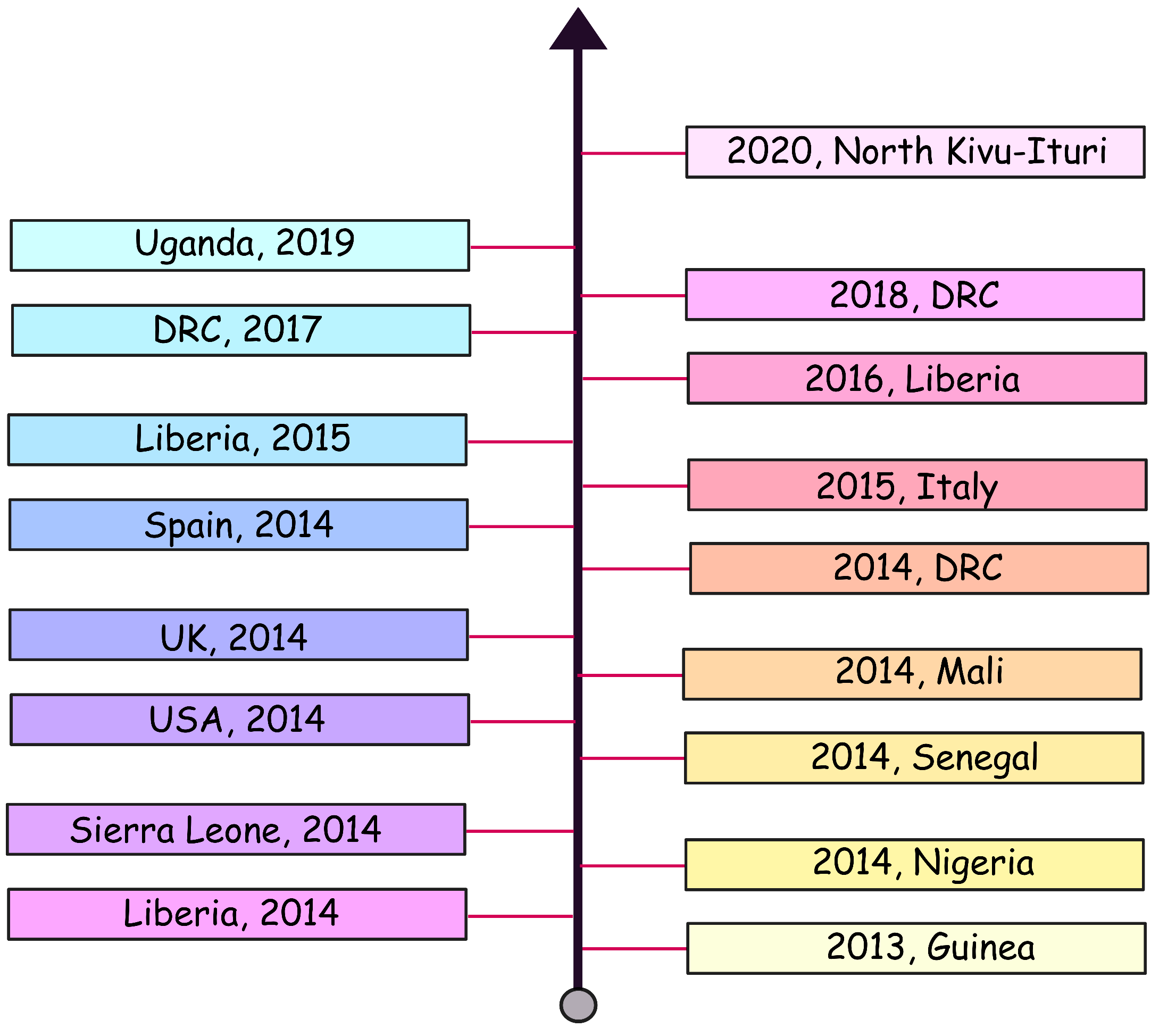
Figure 1. Timeline of the global Ebola virus epidemic between 2013 and 2020.
Fractalfract 06 00578 g001
Figure 2. Fitting of the deterministic model with the Ebola virus statistical data by using the values of parameter from Table 2.
Fractalfract 06 00578 g002
Figure 3. Solutions’ paths and the associated histograms of the Ebola virus model (3) when the numerical values are taken as shown in Table 2 and the random intensities as follows: ϖ s = 0.8 , ϖ e = 2.19 , ϖ q = 0.44 and ϖ r = 0.3 .
Fractalfract 06 00578 g003
Figure 4. Stochastic paths and the associated histograms of the Ebola virus model (3) when the numerical values are taken as shown in Table 2 and the random intensities as follows: ϖ s = 0.05 , ϖ e = 0.09 , ϖ q = 0.04 and ϖ r = 0.03 .
Fractalfract 06 00578 g004
Figure 5. The first row represents the paths of the affected category for the following different time lags: ς 1 = 30 , ς 1 = 100 and ς 1 = 200 . The second row shows the associated histograms and the probability density functions for I s .
Fractalfract 06 00578 g005
Figure 6. The first row represents the paths of the affected category for the following different time lags: ς 2 = 30 , ς 2 = 100 and ς 2 = 200 . The second row shows the associated histograms and the probability density functions for I s .
Fractalfract 06 00578 g006
Figure 7. The first row represents the paths of the affected category for the following different time lags ς 1 = 50 , ς 1 = 150 and ς 1 = 400 . The second row shows the associated histograms and the probability density functions for I s .
Fractalfract 06 00578 g007
Figure 8. The long-run behavior of the Ebola without and with control strategies: (first column) curves achieved from the solution of the deterministic system and (second column) trajectories of the random system.
Fractalfract 06 00578 g008
Figure 9. The curves exhibit the time-evolution of the control measures obtained from simulating the models: deterministic and stochastic.
Fractalfract 06 00578 g009
Table 1. Definition of some subsets used in the demonstration of Theorem 1, where x > Υ > 0 are two constants to be selected later.
SubsetDefinition
W a ( t , ω ) [ ς , [ × Ω | I s ( t , ω ) Υ , and , I e ( t , ω ) Υ
W b ( t , ω ) [ ς , [ × Ω | I s ( t , ω ) Υ
W c ( t , ω ) [ ς , [ × Ω | I e ( t , ω ) Υ
W d { ( t , ω ) [ ς , [ × Ω | I s ( t , ω ) x , or , I e ( t , ω ) x }
W g { ( t , ω ) [ ς , [ × Ω | Υ I s ( t , ω ) x , and , Υ I e ( t , ω ) x }
Table 2. The estimated and fitted values of the parameters obtained from fitting the model against the real Ebola cases reported in Western Guinea from the first forty weeks of the 2015 Ebola epidemic [18].
ParameterEpidemiological MeaningValueSource
A Recruitment rate into susceptible class10Estimated
hThe Ebola transmission rate 0.0004 Fitted
uThe normal death rate of each class 1.2531 × 10 3 Fitted
vThe vaccination rate of the susceptible individuals 0.00027 Estimated
zThe recovery rate of quarantine class 0.13531 Fitted
qThe quarantine rate of infected class 0.802529 Fitted
wThe recovery rate of infectious individuals 0.0209 Fitted
α 1 The disease-related death rate of infected class 1.0135 × 10 6 Fitted
α 2 The disease-related death rate of isolated class 3.1969 × 10 2 Fitted
ς 1 Time delay associated with I s 21Fitted
ς 2 Time delay associated with I e 21Estimated
ς 3 Time delay associated with I q 21Estimated
Publisher’s Note: MDPI stays neutral with regard to jurisdictional claims in published maps and institutional affiliations.