
A Look-Up Table Based Fractional Order Composite Controller Synthesis Method for the PMSM Speed Servo System


Abstract
:1. Introduction
- A composite control scheme is presented, providing the optimal dynamic performance and sufficient robustness for the PMSM speed servo system;
- A look-up table based synthesis method is proposed to simplify the tuning of the optimal controller, creating a wide potential application scope for the proposed method.
2. PMSM Speed Control Problem
- , : d- and q-axis stator currents, respectively;
- , : d and q-axis stator voltages, respectively;
- , : d and q-axis stator inductances, respectively;
- R: stator resistance;
- : pole pairs number;
- : motor angular velocity;
- : magnetic flux linkage;
- J: motor rotating inertia;
- , : friction and load torques, respectively.
3. Fractional Order Composite Control Strategy
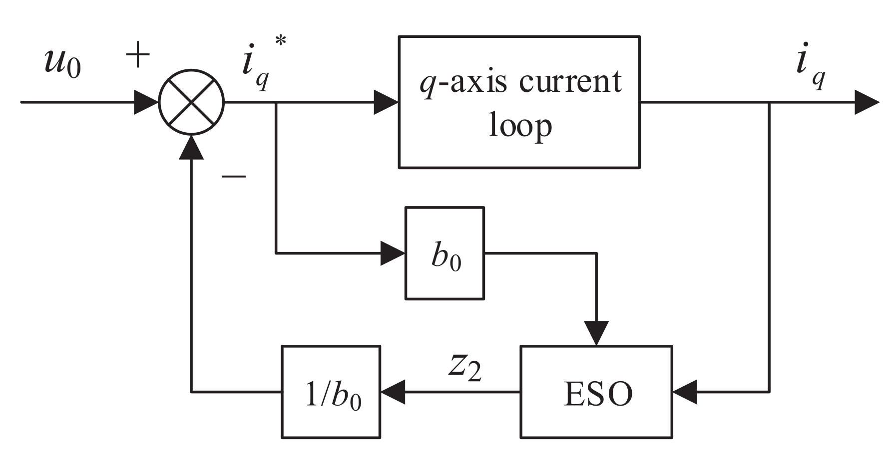
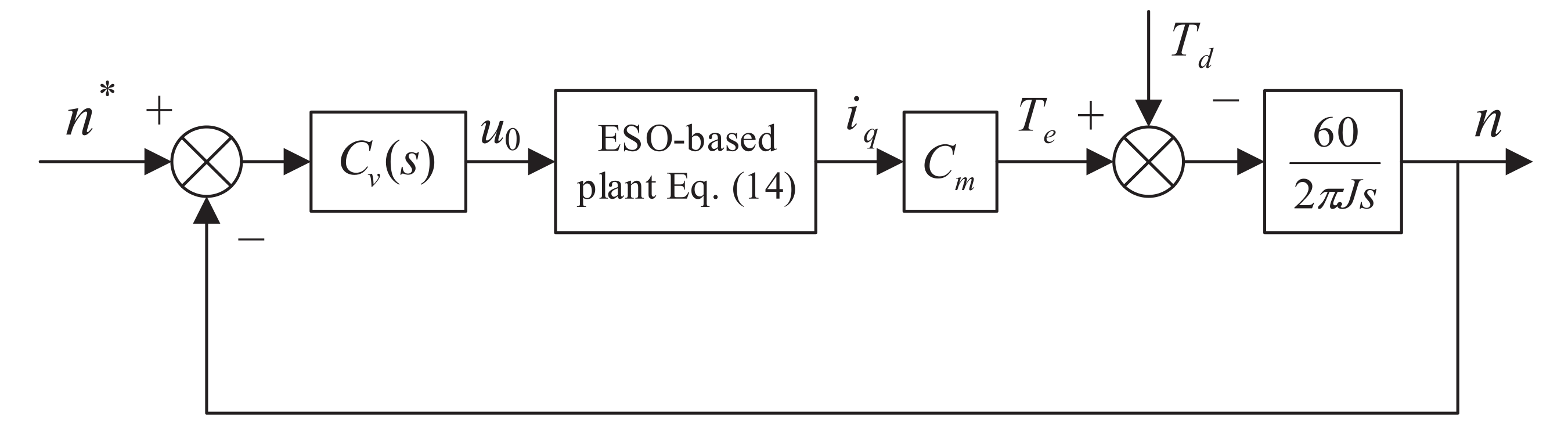
3.1. Eso-Based Composite Control Scheme
3.2. Stability
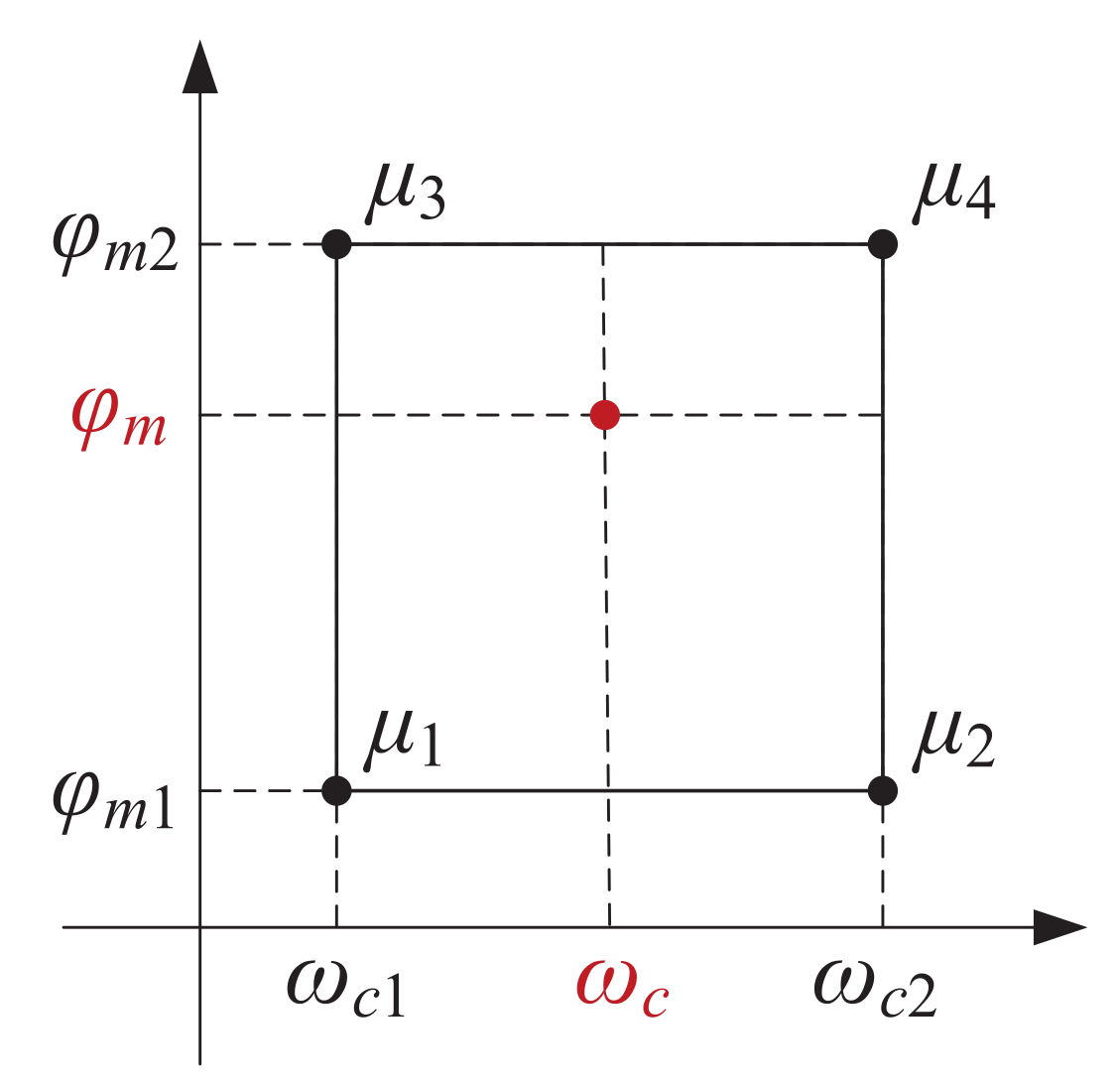
3.3. Optimal Controller Design
4. Application to the PMSM Speed Control Problem
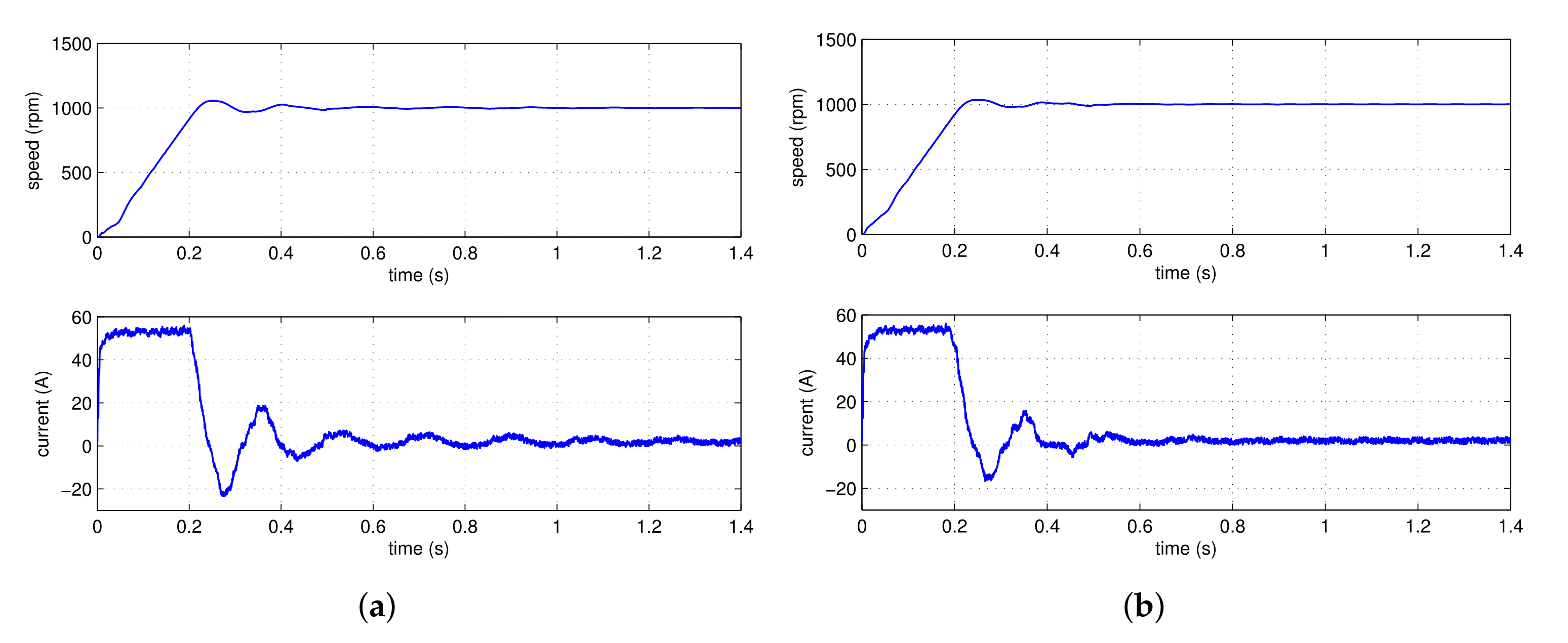
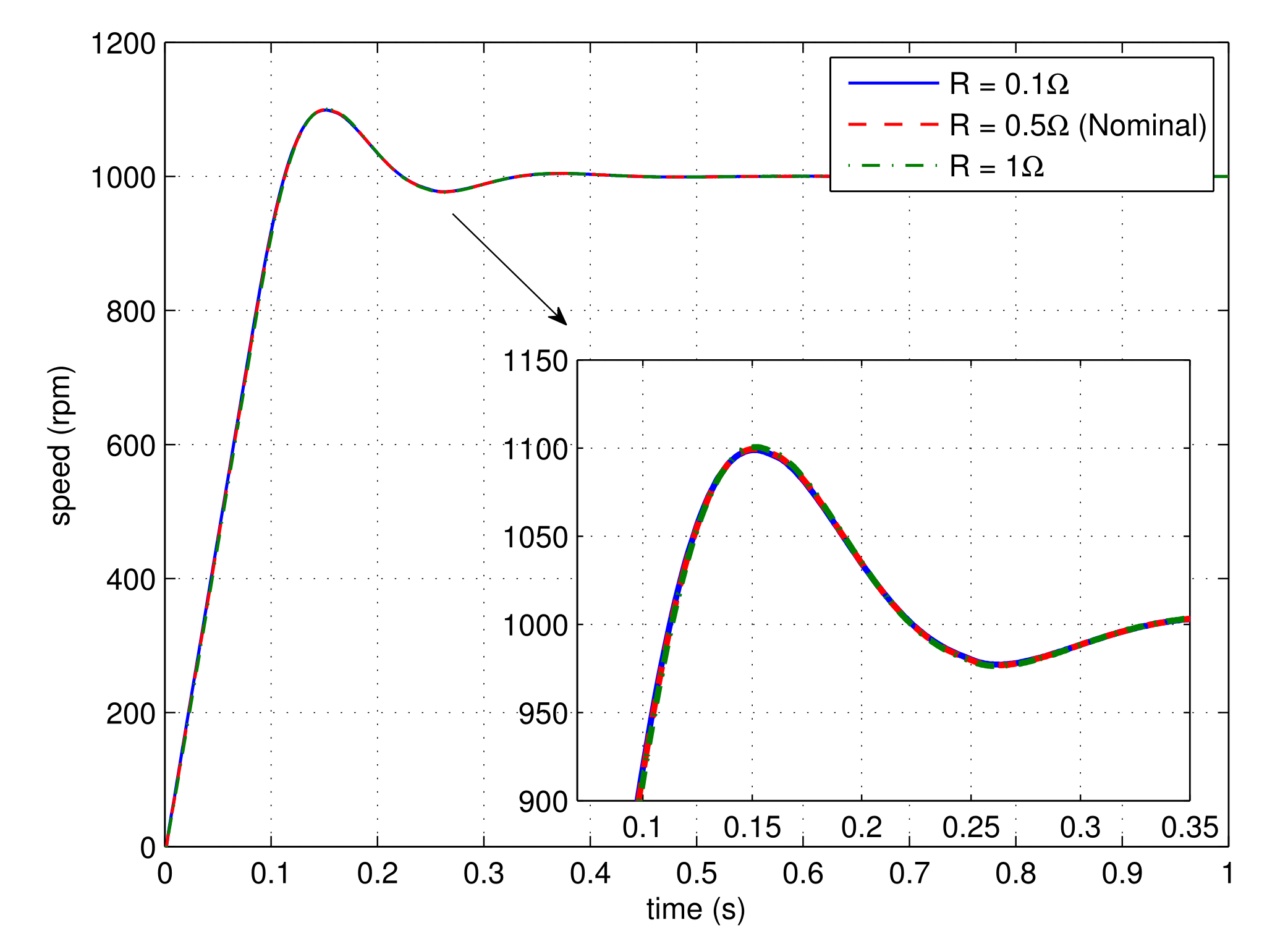
4.1. Simulation Studies
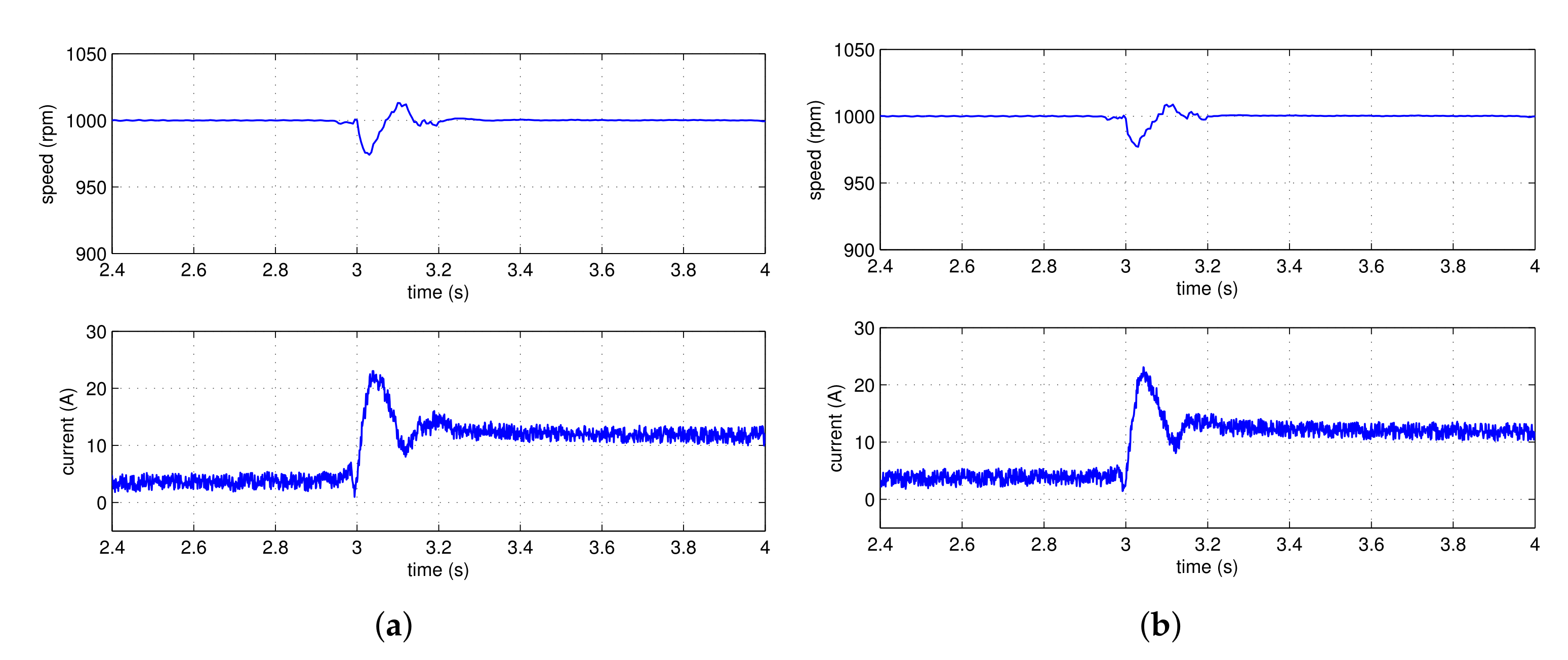
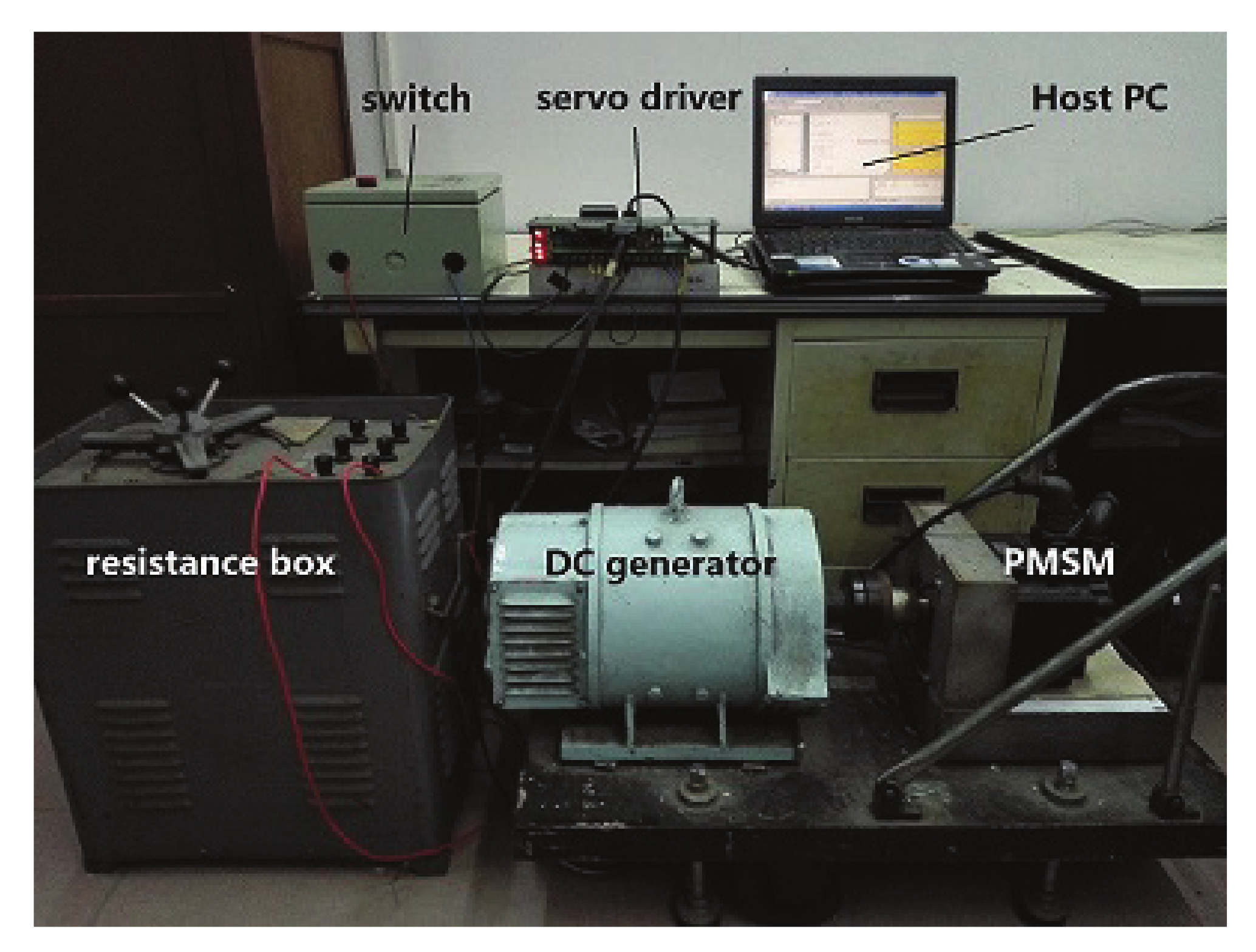
4.2. Experimental Studies
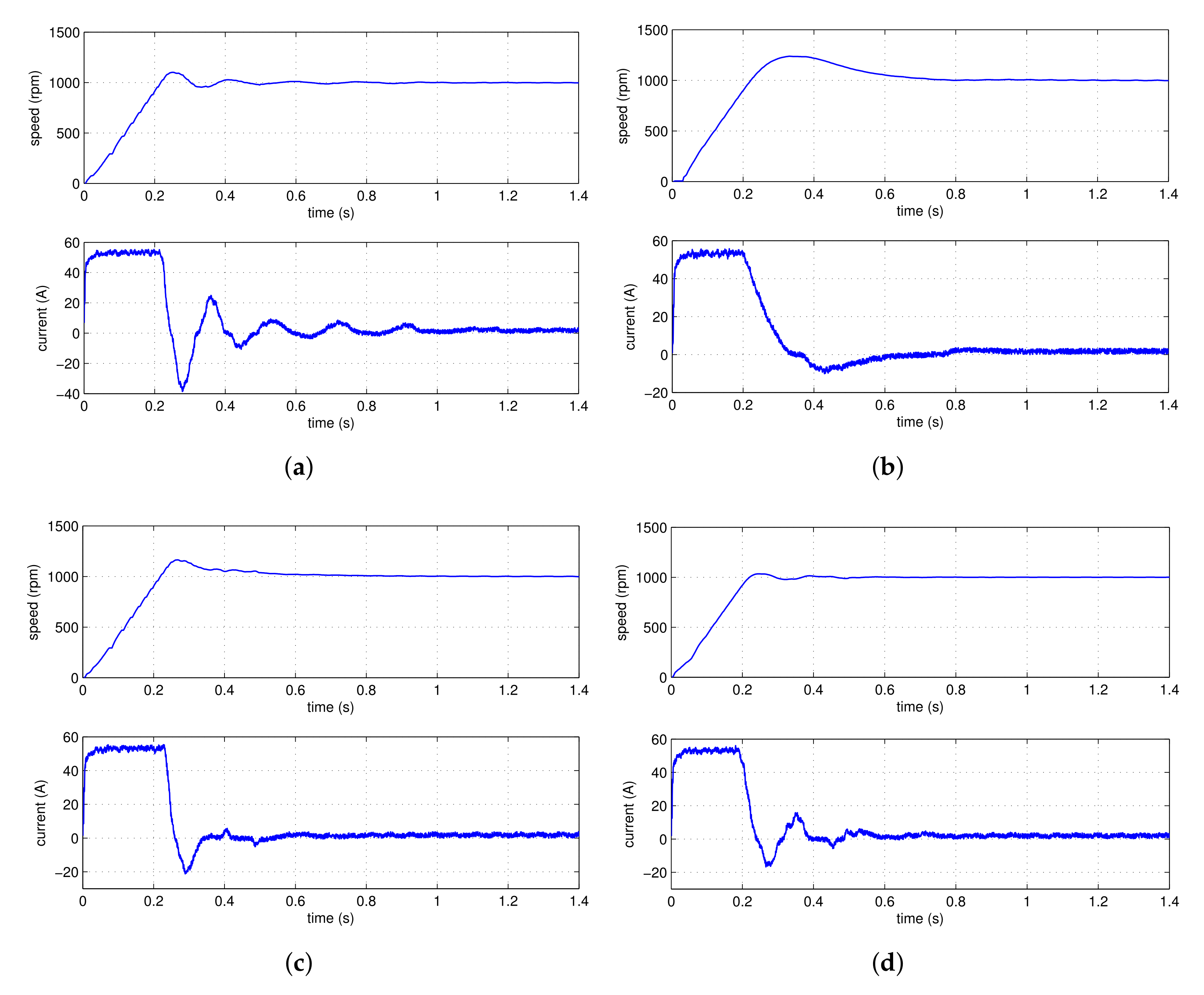
4.2.1. Comparison with the Composite Control Method Using the PD Controller
4.2.2. Comparisons with Some Fractional Order Controllers
5. Conclusions
Author Contributions
Funding
Data Availability Statement
Conflicts of Interest
References
- Wakitani, S.; Yamamoto, T.; Gopaluni, B. Design and application of a database-driven PID controller with data-driven updating algorithm. Ind. Eng. Chem. Res. 2019, 58, 11419–11429. [Google Scholar] [CrossRef]
- Yang, J.; Chen, W.; Li, S.; Guo, L.; Yan, Y. Disturbance/uncertainty estimation and attenuation techniques in PMSM drives—A survey. IEEE Trans. Ind. Electron. 2017, 64, 3273–3285. [Google Scholar] [CrossRef] [Green Version]
- Yan, Y.; Yang, J.; Sun, Z.; Li, S.; Yu, X. Non-linear-disturbance-observer-enhanced MPC for motion control systems with multiple disturbances. IET Control Theory A 2020, 14, 63–72. [Google Scholar] [CrossRef]
- Li, S.; Liu, Z. Adaptive speed control for permanent-magnet synchronous motor system with variations of load inertia. IEEE Trans. Ind. Electron. 2009, 56, 3050–3059. [Google Scholar]
- Chen, D.; Guo, T.; Yang, J.; Li, S. A disturbance observer-based current-constrained controller for speed regulation of PMSM systems subject to unmatched disturbances. IEEE Trans. Ind. Electron. 2021, 68, 767–775. [Google Scholar]
- Yuan, Y.; Wang, Z.; Yang, Y.; Guo, L.; Yang, H. Active disturbance rejection control for a pneumatic motion platform subject to actuator saturation: An extended state observer approach. Automatica 2019, 107, 353–361. [Google Scholar] [CrossRef]
- Ran, M.; Wang, Q.; Dong, C.; Xie, L. Active disturbance rejection control for uncertain time-delay nonlinear systems. Automatica 2020, 112, 108692. [Google Scholar] [CrossRef]
- Haji, V.H.; Monje, C.A. Fractional order fuzzy-PID control of a combined cycle power plant using particle swarm optimization algorithm with an improved dynamic parameters selection. Appl. Soft Comput. 2017, 58, 256–264. [Google Scholar] [CrossRef]
- Shi, L.; Yuan, Y.; Gao, J.; Zhou, L.; Mao, J. Compact fractional-order model of on-chip inductors with BCB on high resistivity silicon. IEEE Trans. Compon. Packag. Manuf. Technol. 2020, 10, 878–886. [Google Scholar] [CrossRef]
- Zheng, W.; Luo, Y.; Chen, Y.; Wang, X. Synthesis of fractional order robust controller based on Bode’s ideas. ISA Trans. 2021, 111, 290–301. [Google Scholar] [CrossRef] [PubMed]
- Shukla, A.; Patel, R. Controllability results for fractional semilinear delay control Systems. J. Appl. Math. Comput. 2021, 65, 861–875. [Google Scholar] [CrossRef]
- Kavitha, K.; Vijayakumar, V.; Udhayakumar, R.; Sakthivel, N.; Nisar, K.S. A note on approximate controllability of the Hilfer fractional neutral differential inclusions with infinite delay. Math. Methods Appl. Sci. 2021, 44, 4428–4447. [Google Scholar] [CrossRef]
- Vijayakumar, V.; Udhayakumar, R. A new exploration on existence of Sobolev-type Hilfer fractional neutral integro-differential equations with infinite delay. Numer. Methods Partial Differ. Equ. 2021, 37, 750–766. [Google Scholar] [CrossRef]
- Raja, M.M.; Vijayakumar, V.; Udhayakumar, R. A new approach on approximate controllability of fractional evolution inclusions of order 1<r<2 with infinite delay, Chaos. Solitons Fractals 2020, 141, 110343. [Google Scholar]
- Ren, H.; Fan, J.; Kaynak, O. Optimal design of a fractional-order proportional-integer-differential controller for a pneumatic position servo system. IEEE Trans. Ind. Electron. 2019, 66, 6220–6229. [Google Scholar] [CrossRef]
- Lin, X.; Liu, J.; Liu, F.; Liu, Z.; Gao, Y.; Sun, G. Fractional-order sliding mode approach of buck converters with mismatched disturbances. IEEE Trans. Circuits Syst. I Regul. Pap. 2021, 68, 3890–3900. [Google Scholar] [CrossRef]
- Zheng, W.; Luo, Y.; Chen, Y.; Wang, X. A simplified fractional order PID controller’s optimal tuning: A case study on a PMSM speed servo. Entropy 2021, 23, 130. [Google Scholar] [CrossRef] [PubMed]
- Shah, P.; Agashe, S. Review of fractional PID controller. Mechatronics 2016, 38, 29–41. [Google Scholar] [CrossRef]
- Sheng, Y.; Bai, W.; Xie, Y. Fractional-order PIλD sliding mode control for hypersonic vehicles with neural network disturbance compensator. Nonlinear Dyn. 2021, 103, 849–863. [Google Scholar] [CrossRef]
- Shi, X.; Chen, Y.; Huang, J. Application of fractional-order active disturbance rejection controller on linear motion system. Control Eng. Pract. 2018, 81, 207–214. [Google Scholar] [CrossRef]
- Liu, L.; Zhang, S.; Chen, Y.; Xue, D. General robustness analysis and robust fractional-order PD controller design for fractional-order plants. IET Control Theory A 2018, 12, 1730–1736. [Google Scholar] [CrossRef] [Green Version]
- Dastjerdi, A.; Saikumar, N.; HosseinNia, S. Tuning guidelines for fractional order PID controllers: Rules of thumb. Mechatronics 2018, 56, 26. [Google Scholar] [CrossRef]
- Malek, H.; Luo, Y.; Chen, Y. Identification and tuning fractional order proportional integral controllers for time delayed systems with a fractional pole. Mechatronics 2013, 23, 746–754. [Google Scholar] [CrossRef]
- Zheng, W.; Luo, Y.; Wang, X.; Pi, Y.; Chen, Y. Fractional order PIλDμ controller design for satisfying time and frequency domain specifications simultaneously. ISA Trans. 2017, 84, 212–222. [Google Scholar] [CrossRef]
- Deng, W.; Liu, H.; Xu, J.; Zhao, H.; Song, Y. An Improved Quantum-Inspired Differential Evolution Algorithm for Deep Belief Network. IEEE Trans. Instrum. Meas. 2020, 69, 7319–7327. [Google Scholar] [CrossRef]
- Ruan, Y.; Yang, Y.; Chen, B. Control System of Electric Drives–Motion Control Systems (In Chinese), 5th ed.; China Machine Press: Beijing, China, 2016. [Google Scholar]
- Tursini, M.; Parasiliti, F.; Zhang, D. Decentralized tracking for a class of interconnected nonlinear systems using variable structure control. IEEE Trans. Ind. Appl. 2002, 38, 1018–1026. [Google Scholar] [CrossRef]
- Lai, C.; Shyu, K. A novel motor drive design for incremental motion system via sliding-mode control method. IEEE Trans. Ind. Electron. 2005, 52, 499–507. [Google Scholar] [CrossRef]
- Gao, Z. Scaling and bandwidth-parameterization based controller tuning. In Proceedings of the 2003 American Control Conference, Denver, CO, USA, 4–6 June 2003; Volume 6, pp. 4989–4996. [Google Scholar]
- Chen, C. Stability. In Linear System Theory and Design, 3rd ed.; Oxford University Press: New York, NY, USA, 1999; pp. 121–125. [Google Scholar]
- Kirk, D.E. Optimal Control Theory: An Introduction; Dover Publications: New York, NY, USA, 2004; pp. 1–3. [Google Scholar]
- Asgharnia, A.; Shahnazi, R.; Jamali, A. Performance and robustness of optimal fractional fuzzy PID controllers for pitch control of a wind turbine using chaotic optimization algorithms. ISA Trans. 2018, 79, 27–44. [Google Scholar] [CrossRef] [PubMed]
- Das, S.; Mullick, S.; Suganthan, P. Recent advances in differential evolution—An updated survey. Swarm Evol. Comput. 2016, 27, 1–3. [Google Scholar] [CrossRef]
- Franklin, G.; Powell, J.; Emami-Naeini, A. Feedback Control of Dynamic Systems, 7th ed.; Pearson Education: London, UK, 2015. [Google Scholar]
- Press, W.; Flannery, B.; Teukolsky, S.; Vetterling, W. Numerical Recipes in C: The Art of Scientific Computing, 2nd ed.; Cambridge University Press: Cambridge, UK, 1993. [Google Scholar]
- Chen, Y. Impulse Response Invariant Discretization of Fractional Order Integrators/Differentiators, Filter Design and Analysis, MATLAB Central. Available online: http://www.mathworks.com/matlabcentral/fileexchange/21342-impulse-response-invariant-discretization-of-fractional-order-integrators-differentiators (accessed on 16 December 2021).
- Ahn, H.; Chen, Y. Necessary and sufficient stability condition of fractional-order interval linear systems. Automatica 2008, 44, 2985–2988. [Google Scholar] [CrossRef]
- Zhang, F.; Yang, C.; Zhou, X.; Gui, W. Fractional-order PID controller tuning using continuous state transition algorithm. Neural Comput. Applic. 2018, 29, 795–804. [Google Scholar] [CrossRef]
- Bettayeb, M.; Mansouri, R. Fractional IMC-PID-filter controllers design for non integer order systems. J. Process Control 2014, 24, 261–271. [Google Scholar] [CrossRef]
- Sabatier, J.; Lanusse, P.; Melchior, P.; Oustaloup, A. Fractional Order Differentiation and Robust Control Design: CRONE, H-Infinity and Motion Control; Springer: Dordrecht, The Netherlands, 2015. [Google Scholar]


| () | (rad/s) | ||||||||||
|---|---|---|---|---|---|---|---|---|---|---|---|
| 30 | 35 | 40 | 45 | 50 | 55 | 60 | 65 | 70 | 75 | 80 | |
| 30 | 0.765 | 0.781 | 0.795 | 0.808 | 0.820 | 0.831 | 0.842 | 0.852 | 0.861 | 0.869 | 0.878 |
| 35 | 0.806 | 0.823 | 0.836 | 0.848 | 0.859 | 0.869 | 0.879 | 0.887 | 0.893 | 0.900 | 0.907 |
| 40 | 0.845 | 0.861 | 0.872 | 0.883 | 0.891 | 0.899 | 0.907 | 0.914 | 0.920 | 0.927 | 0.933 |
| 45 | 0.881 | 0.893 | 0.903 | 0.911 | 0.919 | 0.926 | 0.931 | 0.935 | 0.939 | 0.942 | 0.946 |
| 50 | 0.911 | 0.922 | 0.930 | 0.937 | 0.941 | 0.944 | 0.948 | 0.950 | 0.954 | 0.956 | 0.959 |
| 55 | 0.939 | 0.946 | 0.952 | 0.956 | 0.959 | 0.962 | 0.964 | 0.967 | 0.968 | 0.970 | 0.972 |
| 60 | 0.962 | 0.968 | 0.972 | 0.975 | 0.977 | 0.978 | 0.980 | 0.981 | 0.982 | 0.983 | 0.984 |
| () | (rad/s) | ||||
|---|---|---|---|---|---|
| 35 | 45 | 55 | 65 | 75 | |
| 35 | 0.059% | 0.030% | 0.017% | 0.071% | 0.008% |
| 45 | 0.014% | 0.005% | 0.009% | 0.054% | 0.006% |
| 55 | 0.003% | 0.002% | 0.009% | 0.004% | 0.021% |
| Index | IOPD-ESO | FOPD-ESO |
|---|---|---|
| Settling time (s) | 0.266 | 0.207 |
| Overshoot (%) | 5.51 | 3.41 |
| Index | IOPD-ESO | FOPD-ESO |
|---|---|---|
| Dynamic speed drop (%) | 2.59 | 2.30 |
| Recovery time (s) | 0.122 | 0.052 |
| Index | FOPID-STA | IMC-PID | CRONE | FOPD-ESO |
|---|---|---|---|---|
| Settling time (s) | 0.243 | 0.605 | 0.452 | 0.207 |
| Overshoot (%) | 12.43 | 23.77 | 16.40 | 3.41 |
| Index | FOPID | IMC-PID | CRONE | FOPD-ESO |
|---|---|---|---|---|
| Dynamic speed drop (%) | 2.26 | 6.65 | 2.42 | 2.30 |
| Recovery time (s) | 0.108 | 0.372 | 0.143 | 0.052 |
Publisher’s Note: MDPI stays neutral with regard to jurisdictional claims in published maps and institutional affiliations. |
© 2022 by the authors. Licensee MDPI, Basel, Switzerland. This article is an open access article distributed under the terms and conditions of the Creative Commons Attribution (CC BY) license (https://creativecommons.org/licenses/by/4.0/).
Share and Cite
Zheng, W.; Huang, R.; Luo, Y.; Chen, Y.; Wang, X.; Chen, Y. A Look-Up Table Based Fractional Order Composite Controller Synthesis Method for the PMSM Speed Servo System. Fractal Fract. 2022, 6, 47. https://doi.org/10.3390/fractalfract6010047
Zheng W, Huang R, Luo Y, Chen Y, Wang X, Chen Y. A Look-Up Table Based Fractional Order Composite Controller Synthesis Method for the PMSM Speed Servo System. Fractal and Fractional. 2022; 6(1):47. https://doi.org/10.3390/fractalfract6010047
Chicago/Turabian StyleZheng, Weijia, Runquan Huang, Ying Luo, YangQuan Chen, Xiaohong Wang, and Yong Chen. 2022. "A Look-Up Table Based Fractional Order Composite Controller Synthesis Method for the PMSM Speed Servo System" Fractal and Fractional 6, no. 1: 47. https://doi.org/10.3390/fractalfract6010047
APA StyleZheng, W., Huang, R., Luo, Y., Chen, Y., Wang, X., & Chen, Y. (2022). A Look-Up Table Based Fractional Order Composite Controller Synthesis Method for the PMSM Speed Servo System. Fractal and Fractional, 6(1), 47. https://doi.org/10.3390/fractalfract6010047