
A Novel Treatment of Fuzzy Fractional Swift–Hohenberg Equation for a Hybrid Transform within the Fractional Derivative Operator


Abstract
:1. Introduction
2. Prelude
- 1.
- ∇ is normal (for some );
- 2.
- ∇ is upper semi continuous;
- 3.
- i.e., ∇ is a convex fuzzy set;
- 4.
- is compact.
- 1.
- is nondecreasing, left continuous, bounded over and right continuous at ;
- 2.
- is nonincreasing, left continuous, bounded over and right continuous at ;
- 3.
- 1.
- 2.
- 3.
- I.
- and are differentiable, if Λ is a (1)-differentiable, and
- II.
- and are differentiable, if Λ is a (2)-differentiable, and
- differentiable:
- differentiable:which are defined as the subsequent form for
3. Analysis of CFD Operator in View of Elzaki Transform
- differentiability:
- differentiability:
4. Analysis Description
5. Convergence Analysis of Fuzzy EADM
- (i)
- The mappings are equicontinuous and uniformly bounded on any bounded set;
- (ii)
- There exist such that
- (i)
- (ii)
6. Numerical Findings and Their Physical Evaluation
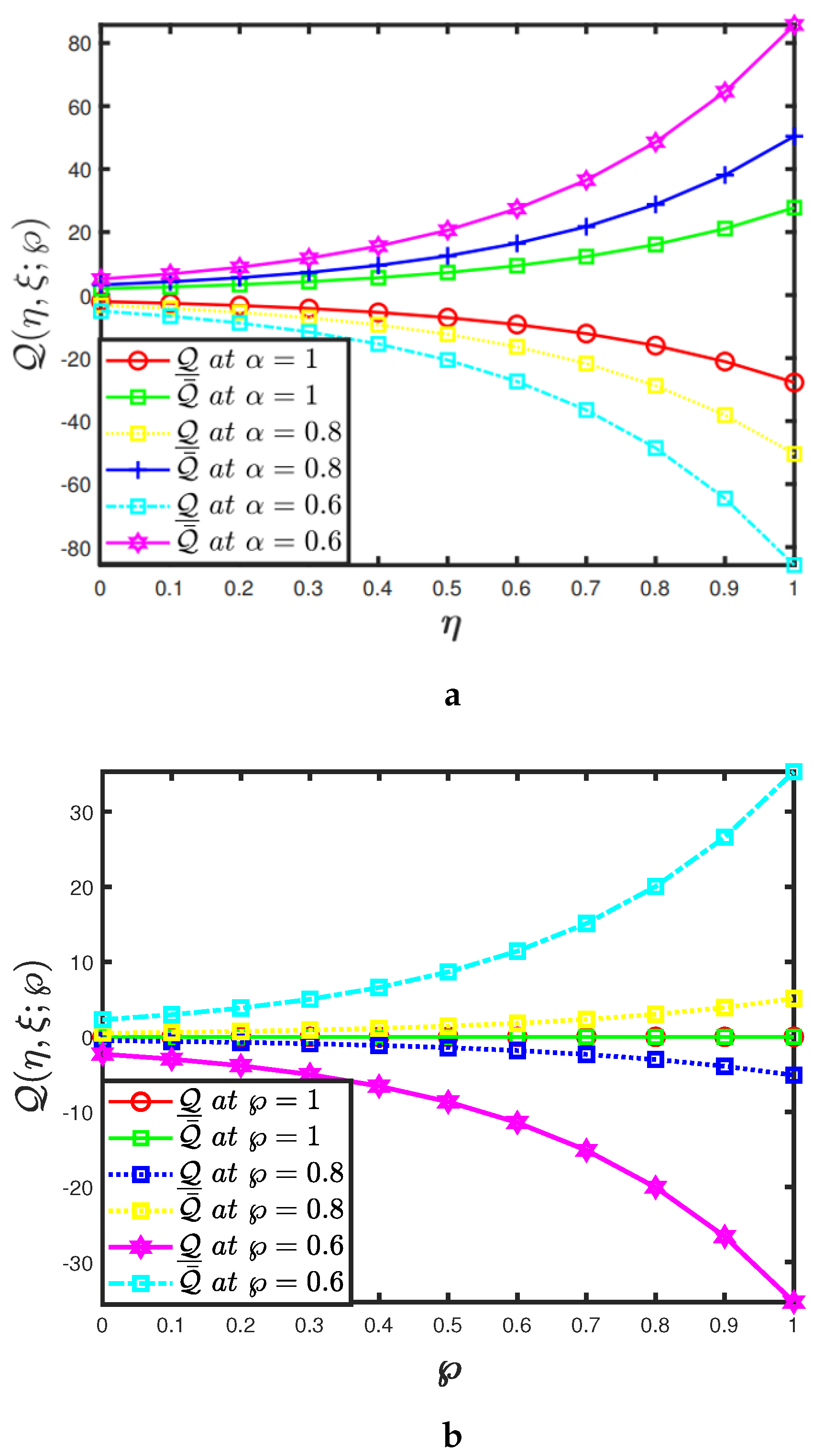
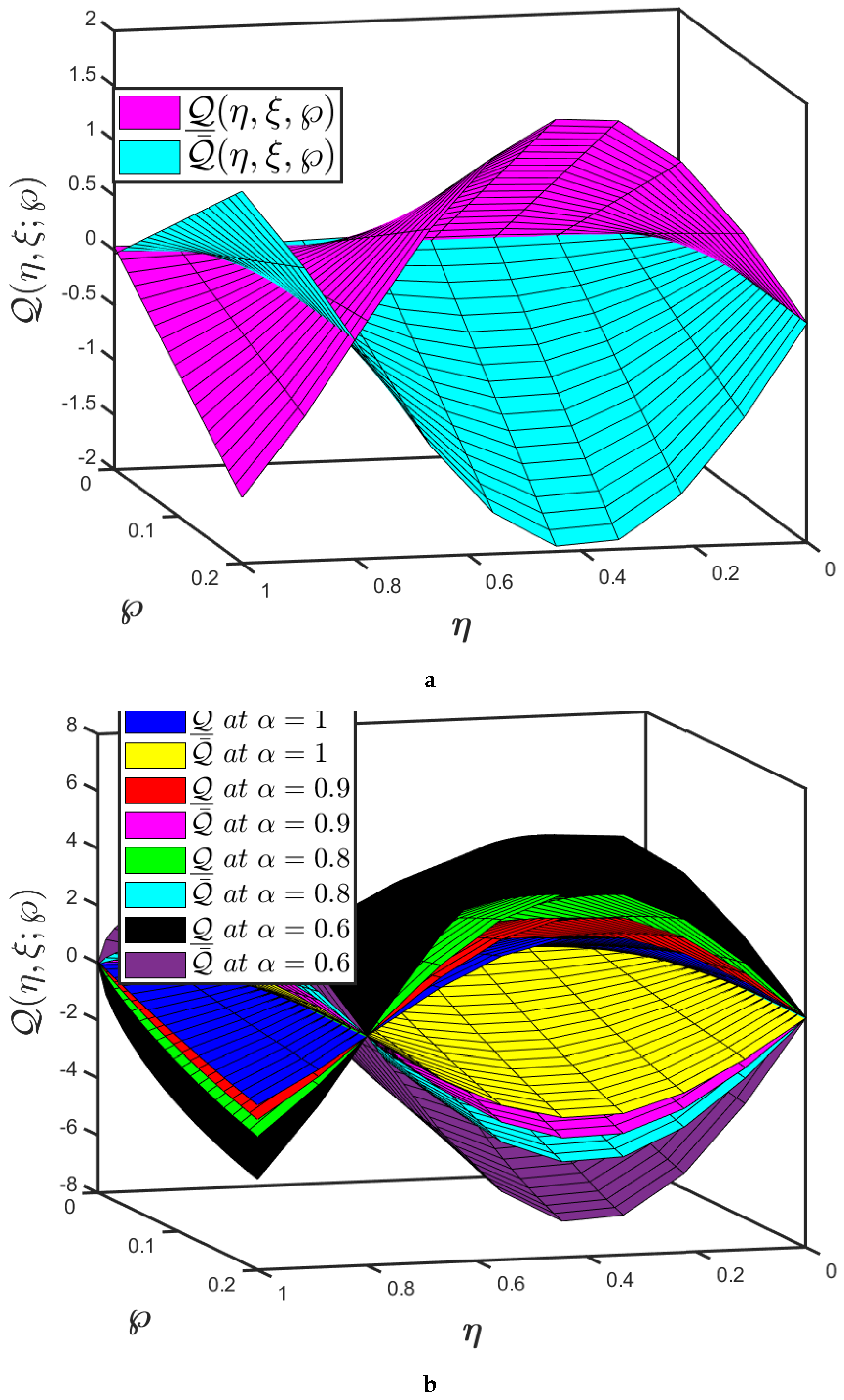
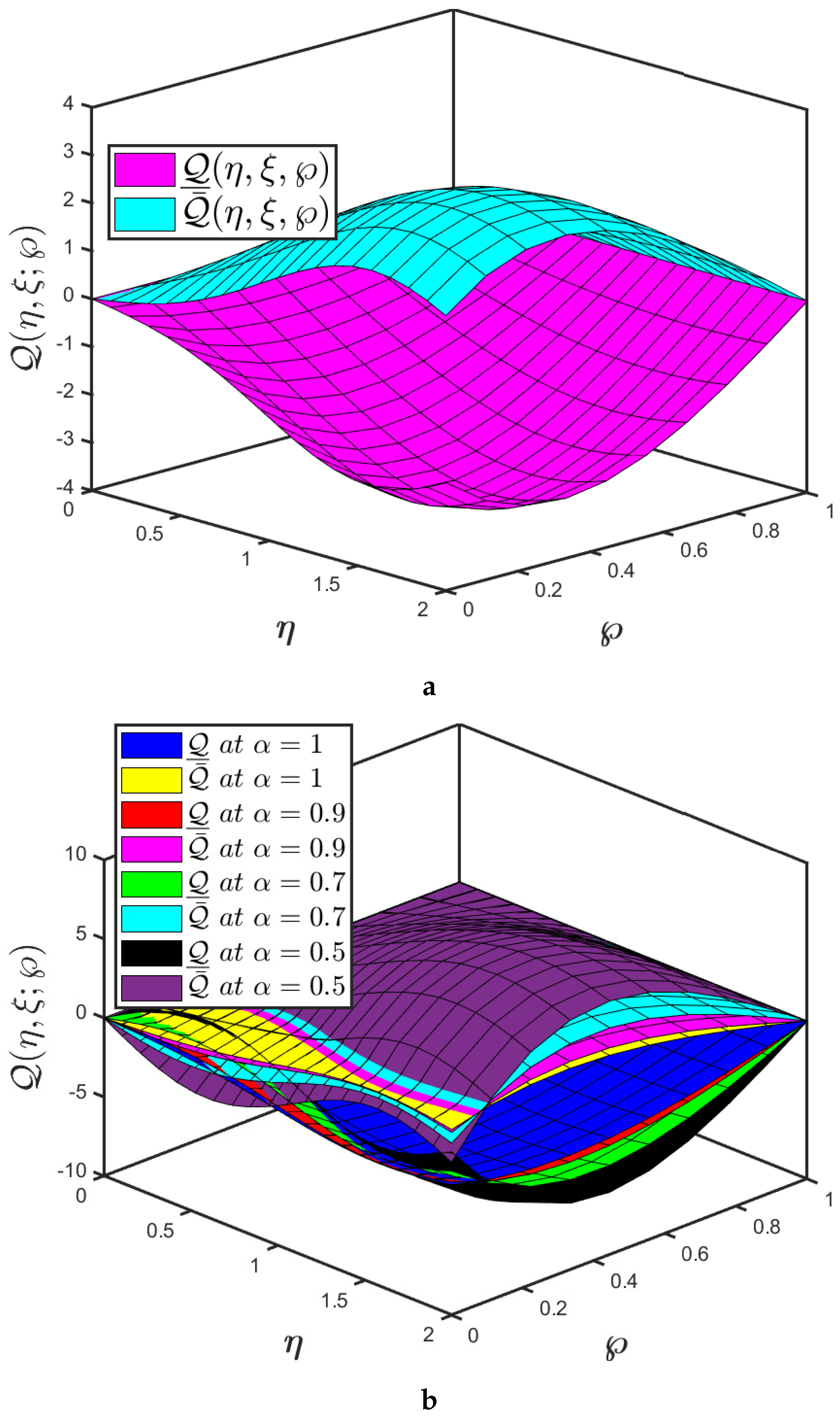
- The mapping effectiveness of the suggested algorithm, is displayed in Figure 2a for the constant parameter The analysis demonstrates a minor improvement in with the decrease in ;
- The uncertainty parameter of the mappings and are presented in Figure 2a,b and it elaborates the behaviour of the specified fractional order of the mapping at various uncertainty parameters;
- The aforementioned graphs presented in Figure 1 and Figure 2 assist us in comprehending the statistical behaviour of time and space variation. Furthermore, the offered approach will aid scientists working in pattern formation theory, optical design, and statistical dynamics in evaluating performance through analysis of variance testing. As a result, the uncertainty parameter can strengthen the results after increasing the number of iterations.

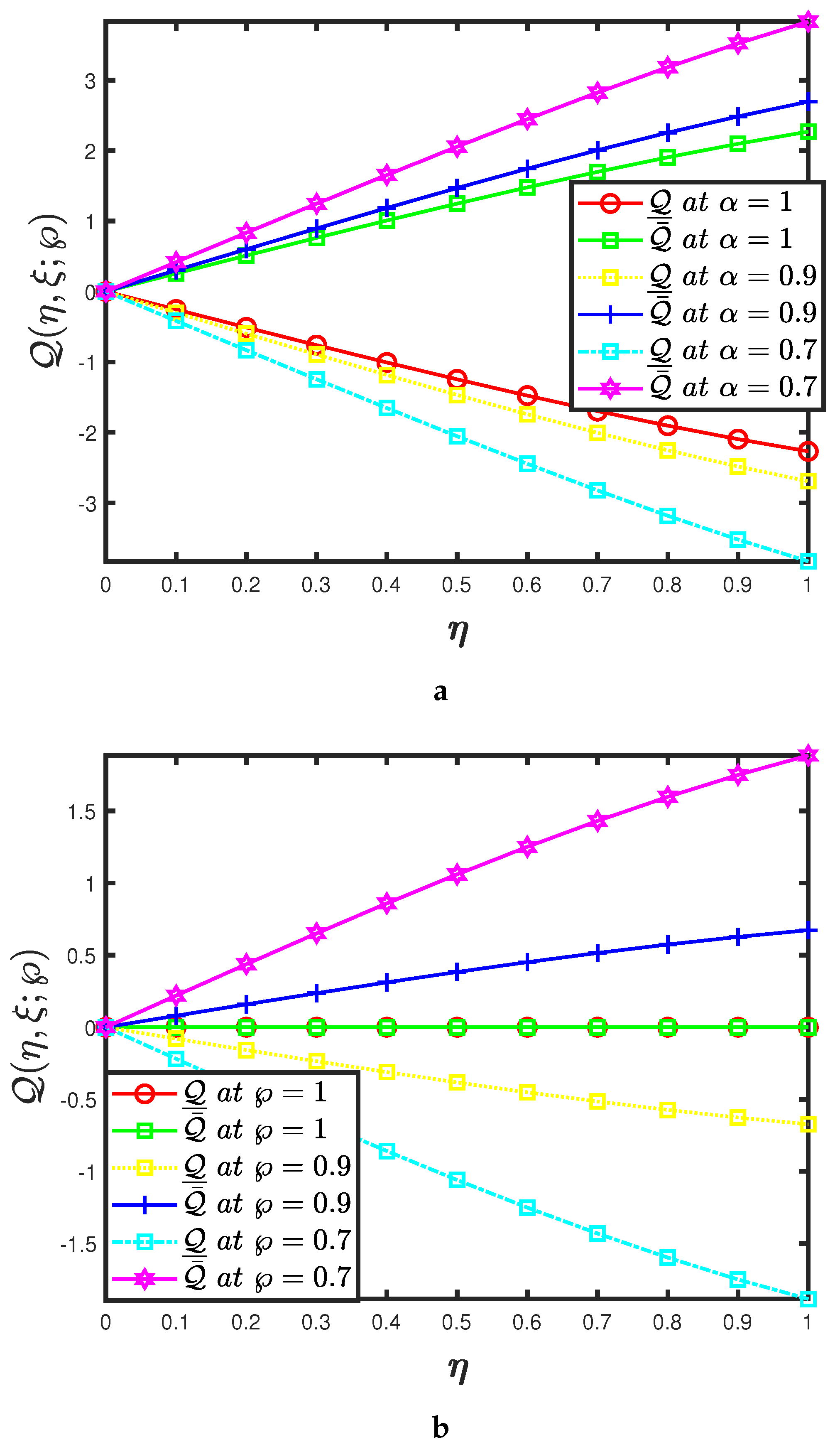
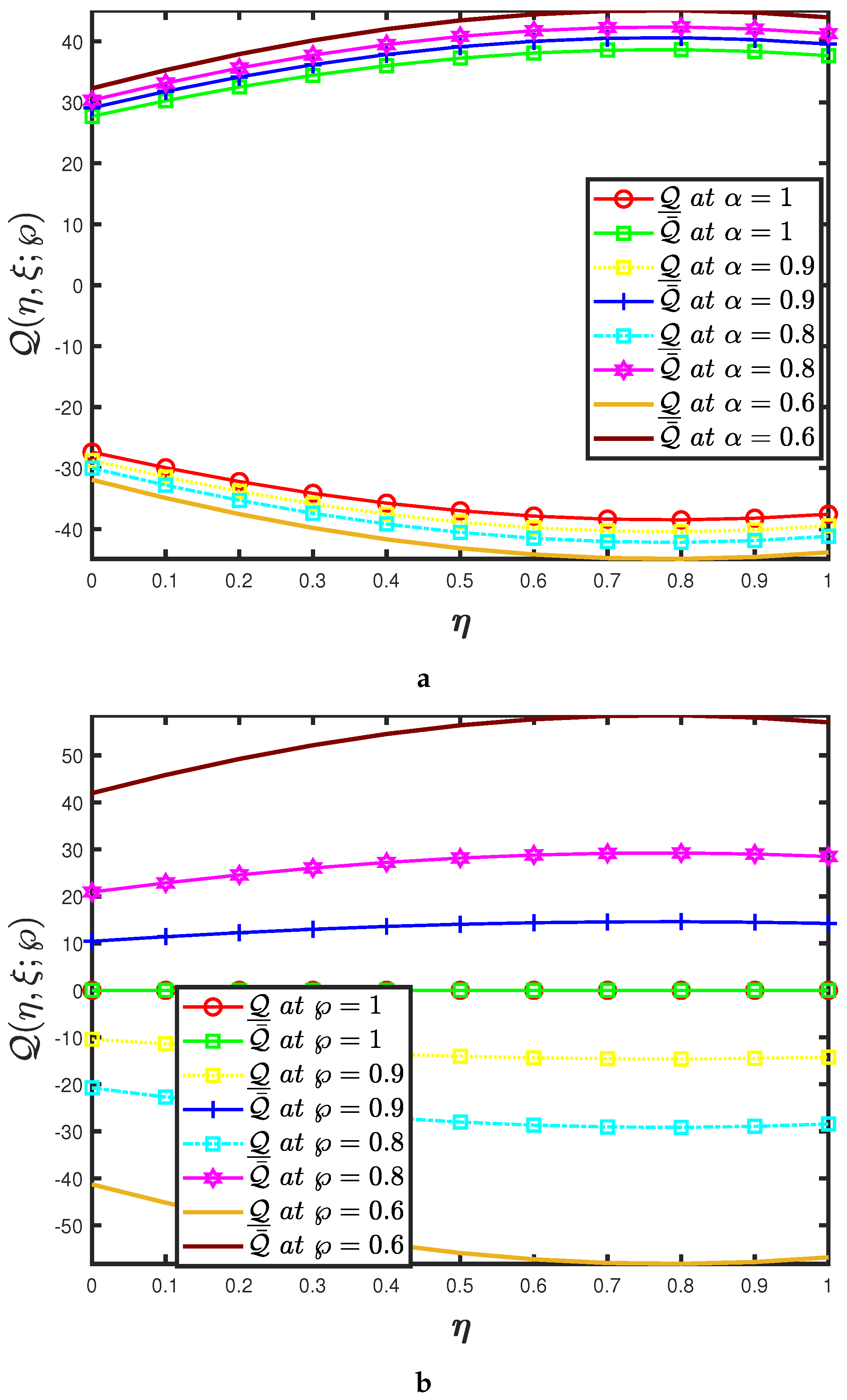
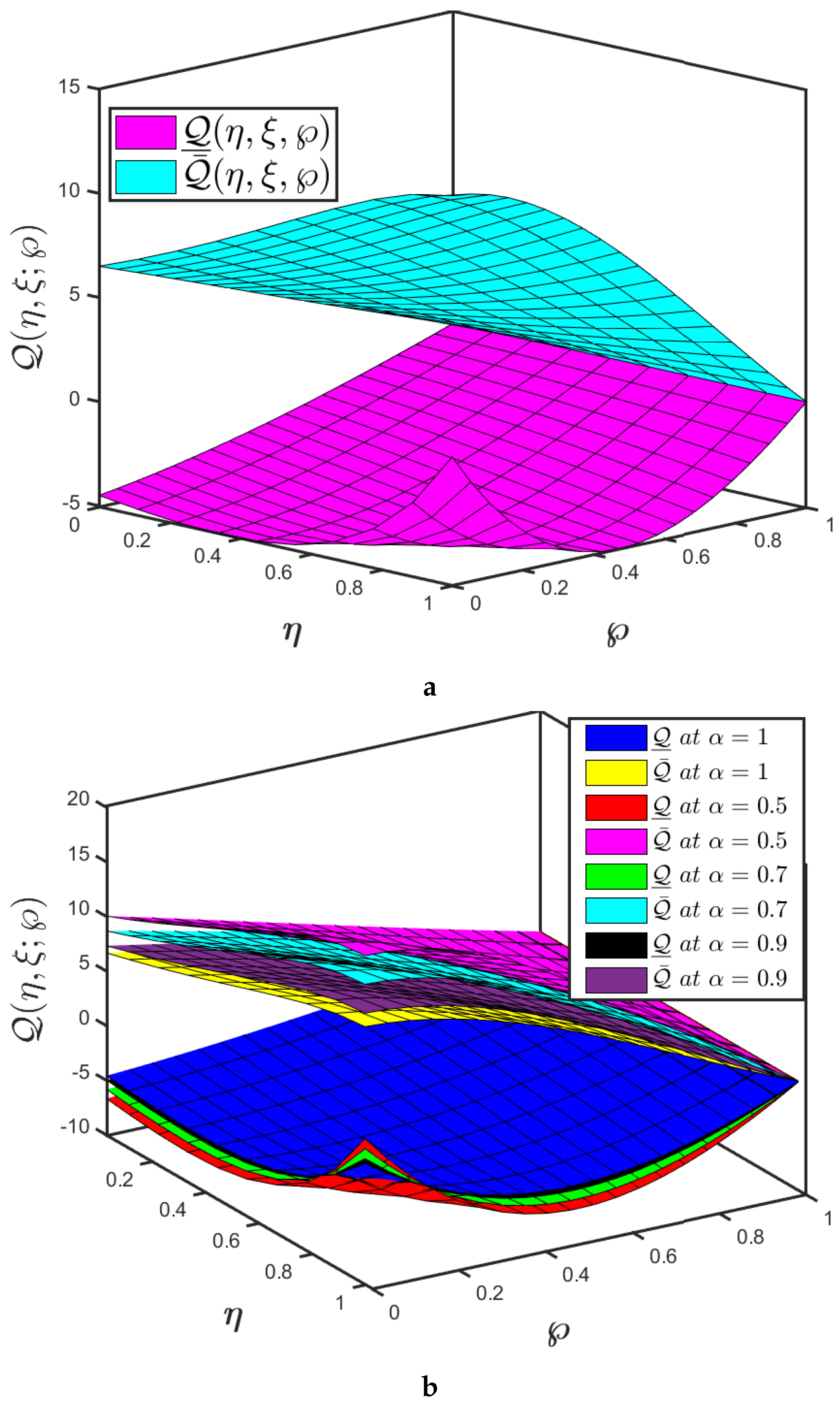
- The mapping effectiveness of the suggested algorithm, is displayed in Figure 4a for the constant parameter The analysis demonstrates a minor improvement in with the decrease in ;
- The uncertainty parameter of the mappings and are presented in Figure 4a,b and it elaborates the behaviour of specified fractional order of the mapping at various uncertainty parameters;

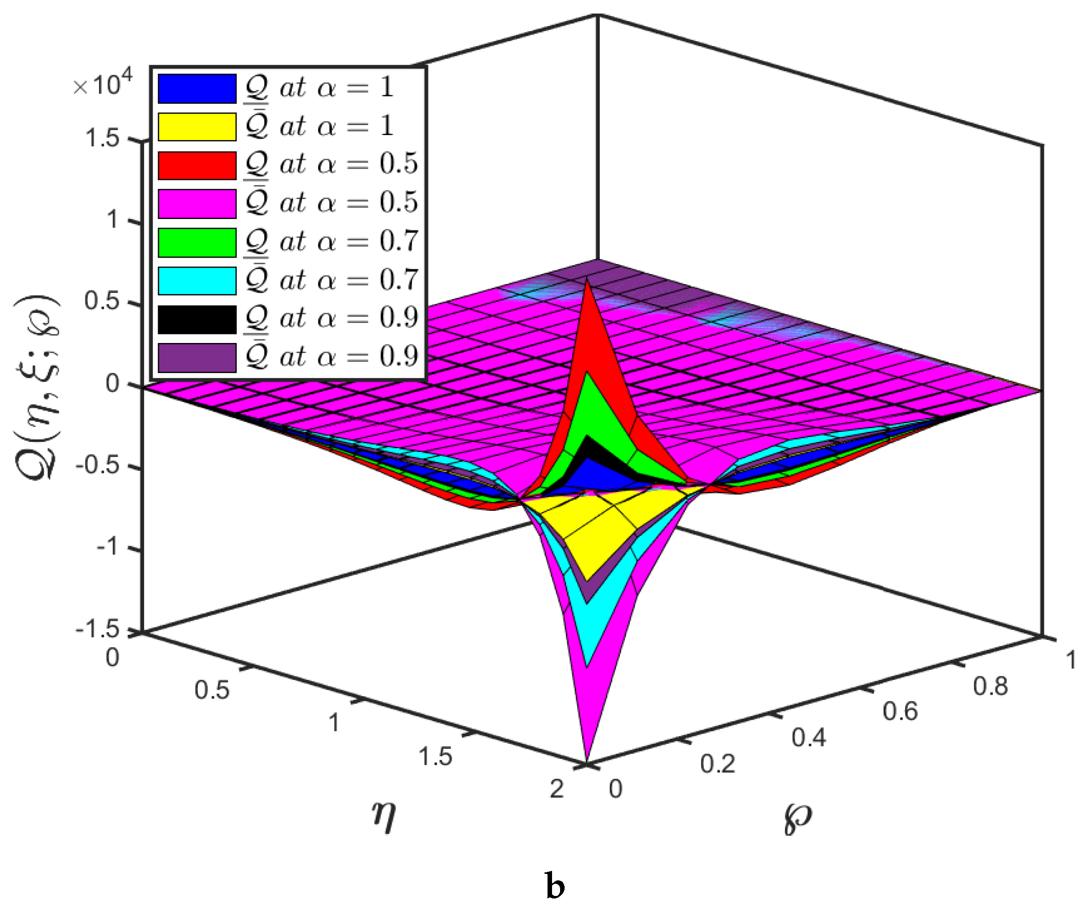
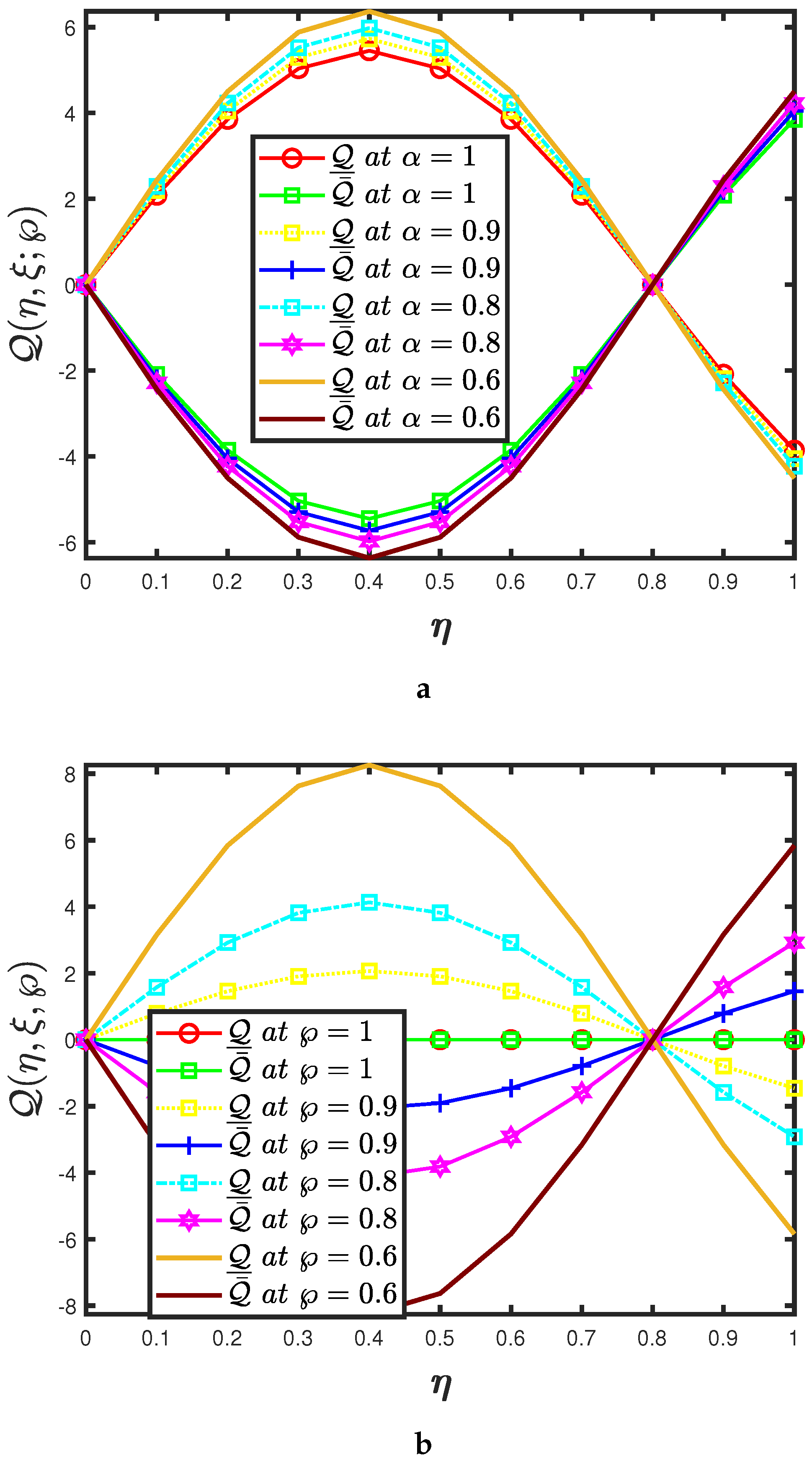
- The mapping effectiveness of the suggested algorithm, is displayed in Figure 6a for the constant parameter and The analysis demonstrates a minor improvement in with the decrease in ;
- The uncertainty parameter of the mappings and are presented in Figure 6a,b and it elaborates the behaviour of specified fractional order of the mapping at various uncertainty parameters.

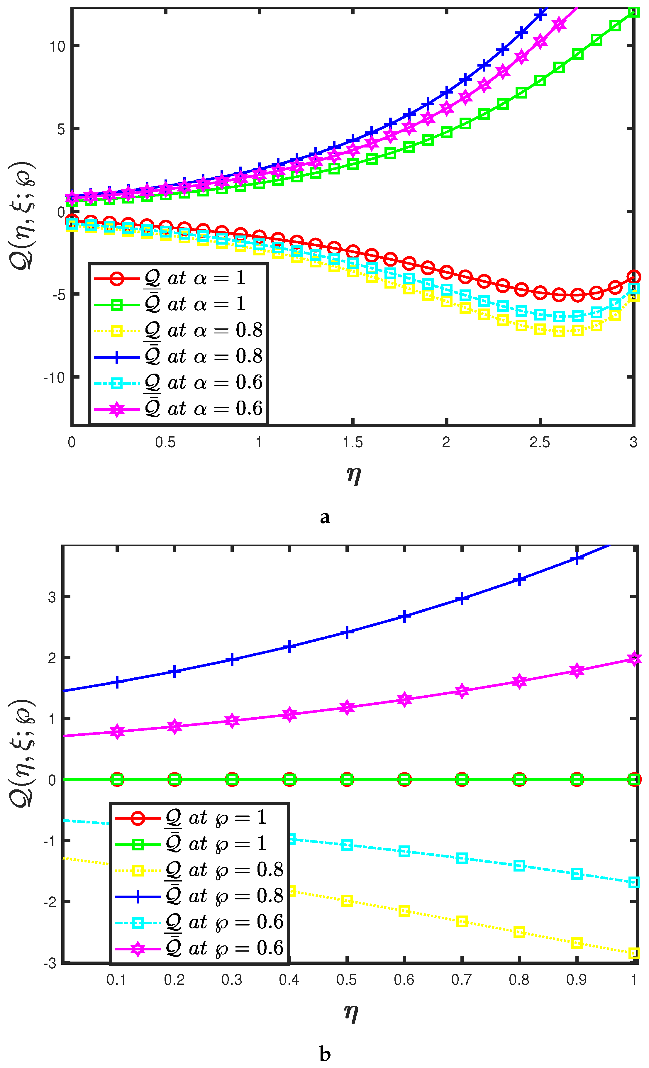
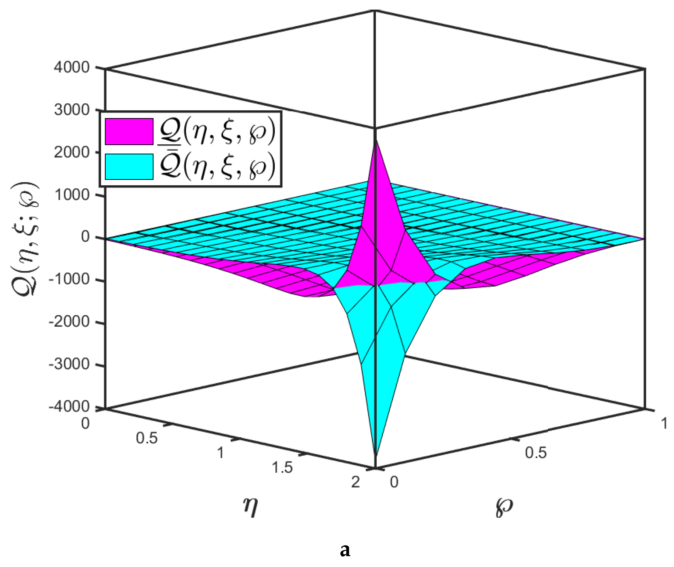
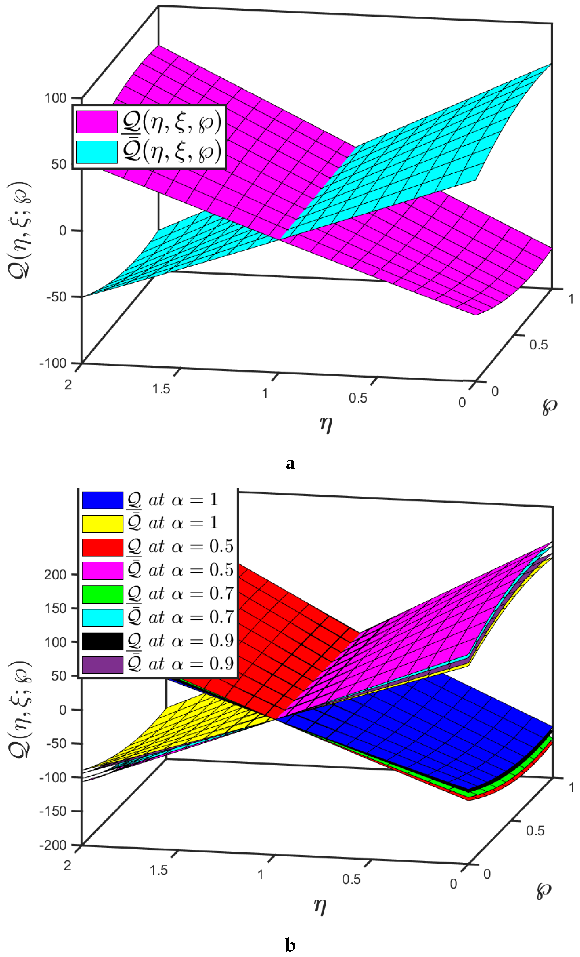
- The mapping effectiveness of the suggested algorithm, is displayed in Figure 8a for the constant parameter and The analysis demonstrates a minor improvement in with the decrease in .
- The uncertainty parameter of the mappings and are presented in Figure 8a,b and it elaborates the behaviour of specified fractional order of the mapping at various uncertainty parameters.
- With these findings, the qualitative resemblance of the cross patterns created to those occurring in nature, such as Rayleigh–Bénard convection, may be confirmed. Despite the various factors that initiate and enhance the instability, pattern development is the consequence of self-organization systems, and all of these are good instances of this phenomena.
- The mapping effectiveness of the suggested algorithm, is displayed in Figure 10a for the constant parameter and . The analysis demonstrates a minor improvement in with the decrease in ;
- The uncertainty parameter of the mappings and are presented in Figure 10a,b and it elaborates the behaviour of specified fractional order of the mapping at various uncertainty parameters;
- The nature of the probability density function is controlled by dispersion, fractional order and uncertainty parameters, according to these findings. The behaviour of hydrodynamic stability is defined by the oscillatory wave patterns of the bifurcation parameter. Further, (5) describes the convective describes the convective heat current in a Rayleigh–Bénard cell and the nature of hydrodynamic stability.
7. Conclusions
Author Contributions
Funding
Institutional Review Board Statement
Informed Consent Statement
Data Availability Statement
Acknowledgments
Conflicts of Interest
References
- Podlubny, I. Fractional Differential Equations; Academic Press: San Diego, CA, USA, 1999. [Google Scholar]
- Hilfer, R. Applications of Fractional Calculus in Physics; Word Scientific: Singapore, 2000. [Google Scholar]
- Kilbas, A.; Srivastava, H.M.; Trujillo, J.J. Theory and Application of Fractional Differential Equations; Elsevier: Amsterdam, The Netherlands, 2006; Volume 204, pp. 1–523. [Google Scholar]
- Magin, R.L. Fractional Calculus in Bioengineering; Begell House Publishers: Redding, CT, USA, 2006. [Google Scholar]
- Samko, S.G.; Kilbas, A.A.; Marichev, O.I. Fractional Integrals and Derivatives: Theory and Applications; Gordon and Breach: Yverdon, Switzerland, 1993. [Google Scholar]
- Alqudah, M.A.; Ashraf, R.; Rashid, S.; Singh, J.; Hammouch, Z.; Abdeljawad, T. Novel numerical investigations of fuzzy Cauchy reaction-diffusion models via generalized fuzzy fractional derivative operators. Fractal Fract. 2021, 5, 151. [Google Scholar] [CrossRef]
- Rashid, S.; Ashraf, R.; Akdemir, A.O.; Alqudah, M.A.; Abdeljawad, T.; Mohamed, M.S. Analytic fuzzy formulation of a time-fractional Fornberg–Whitham model with power and Mittag–Leffler kernels. Fractal Fract. 2021, 5, 113. [Google Scholar] [CrossRef]
- Rashid, S.; Kubra, K.T.; Jafari, H.; Lehre, S.U. A semi-analytical approach for fractional order Boussinesq equation in a gradient unconfined aquifers. Math. Meth. Appl. Sci. 2021, 1–30. [Google Scholar] [CrossRef]
- Rashid, S.; Hammouch, Z.; Aydi, H.; Ahmad, A.G.; Alsharif, A.M. Novel computations of the time-fractional Fisher’s model via generalized fractional integral operators by means of the Elzaki transform. Fractal Fract. 2021, 5, 94. [Google Scholar] [CrossRef]
- Rashid, S.; Kubra, K.T.; Guirao, J.L.G. Construction of an approximate analytical solution for multi-dimensional fractional Zakharov-Kuznetsov equation via Aboodh Adomian decomposition method. Symmetry 2021, 13, 1542. [Google Scholar] [CrossRef]
- Rashid, S.; Kubra, K.T.; Abualnaja, K.M. Fractional view of heat-like equations via the Elzaki transform in the settings of the Mittag-Leffler function. Math. Meth. Appl. Sci. 2021, 1–26. [Google Scholar] [CrossRef]
- Zhou, S.-S.; Rashid, S.; Rauf, A.; Kubra, K.T.; Alsharif, A.M. Initial boundary value problems for a multi-term time fractional diffusion equation with generalized fractional derivatives in time. AIMS Math. 2021, 6, 12114–12132. [Google Scholar] [CrossRef]
- Rashid, S.; Khalid, A.; Sultana, S.; Hammouch, Z.; Shah, R.; Alsharif, A.M. A novel analytical view of time-fractional Korteweg-De Vries equations via a new integral transform. Symmetry 2021, 13, 1254. [Google Scholar] [CrossRef]
- Rashid, S.; Kubra, K.T.; Lehre, S.U. Fractional spatial diffusion of a biological population model via a new integral transform in the settings of power and Mittag-Leffler nonsingular kernel. Phys. Scr. 2021, 96, 114003. [Google Scholar] [CrossRef]
- Rashid, S.; Jarad, F.; Abualnaja, K.M. On fuzzy Volterra-Fredholm integrodifferential equation associated with Hilfer-generalized proportional fractional derivative. AIMS Math. 2021, 6, 10920–10946. [Google Scholar] [CrossRef]
- Abdel-Gawad, H.I.; Osman, M.S. On the variational approach for analyzing the stability of solutions of evolution equations. Kyungpook Math. J. 2013, 53, 661–680. [Google Scholar] [CrossRef] [Green Version]
- Kumar, S.; Kumar, R.; Osman, M.S.; Samet, B. A wavelet based numerical scheme for fractional order SEIR epidemic of measles by using Genocchi polynomials. Numer. Methods Partial. Differ. Equations 2021, 37, 1250–1268. [Google Scholar] [CrossRef]
- Chang, S.L.; Zadeh, L.A. On fuzzy mapping and control. IEEE Trans. Syst. Man Cybern. 1972, 2, 30–34. [Google Scholar] [CrossRef]
- Dubois, D.; Prade, H. Towards fuzzy differential calculus part 3: Differentiation. Fuzzy Sets Syst. 1982, 8, 225–233. [Google Scholar] [CrossRef]
- Kandel, A.; Byatt, W.J. Fuzzy differential equations. In Proceedings of the International Conference Cybernetics and Society, Tokyo, Japan, 3–7 November 1978; pp. 1213–1216. [Google Scholar]
- Agarwal, R.P.; Lakshmikantham, V.; Nieto, J.J. On the concept of solution for fractional differential equations with uncertainty. Nonlinear Anal. Theory Meth. Appl. 2010, 72, 2859–2862. [Google Scholar] [CrossRef]
- El-Sayed, S.; Kaya, D. An application of the ADM to seven-order Sawada-Kotara equations. Appl. Math. Comput. 2004, 157, 93–101. [Google Scholar] [CrossRef]
- Javan, S.F.; Abbasb, Y.S.; Araghi, M.A.F. Application of reproducing kernel Hilbert space method for solving a class of nonlinear integral equations. Math. Prob. Eng. 2017, 2017, 7498136. [Google Scholar] [CrossRef]
- Rao, T.M.R. Application of residual power series method to time fractional gas dynamics equations. J. Phys. Conf. Ser. 2018, 1139, 012007. [Google Scholar]
- Shiralashetti, S.C.; Kumbinarasaiah, S. Laguerre wavelets collocation method for the numerical solution of the Benjamina–Bona–Mohany equations. J. Taibah Univ. Sci. 2019, 13. [Google Scholar] [CrossRef] [Green Version]
- AliaK, A.H.A.; Raslan, R. Variational iteration method for solving partial differential equations with variable coefficients. Chaos Solitons Fractals 2009, 43, 1520–1529. [Google Scholar]
- Hoa, N.V.; Vu, H.; Duc, T.M. Fuzzy fractional differential equations under Caputo Katugampola fractional derivative approach. Fuzzy Sets Syst. 2019, 375, 70–99. [Google Scholar] [CrossRef]
- Hoa, N.V. Fuzzy fractional functional differential equations under Caputo gH-differentiability Commun. Nonlinear Sci. Numer. Simul. 2015, 22, 1134–1157. [Google Scholar] [CrossRef]
- Salahshour, S.; Ahmadian, A.; Senu, N.; Baleanu, D.; Agarwal, P. On analytical aolutions of the fractional differential equation with uncertainty: Application to the Basset problem. Entropy 2015, 17, 885–902. [Google Scholar] [CrossRef] [Green Version]
- Arqub, O.A.; Al-Smadi, M.; Momani, S.; Hayat, T. Application of reproducing kernel algorithm for solving second-order, two-point fuzzy boundary value problems. Soft Comput. 2017, 21, 7191–7206. [Google Scholar] [CrossRef]
- Arqub, O.A. Adaptation of reproducing kernel algorithm for solving fuzzy Fredholm-Volterra integrodifferential equations. Neural Comput. Appl. 2017, 28, 1591–1610. [Google Scholar] [CrossRef]
- Ahmad, S.; Ullah, A.; Akgül, A.; Abdeljawad, T. Semi-analytical solutions of the 3rd order fuzzy dispersive partial differential equations under fractional operators. Alex. Eng. J. 2021, 60, 5861–5878. [Google Scholar] [CrossRef]
- Shah, K.; Seadawy, A.R.; Arfan, M. Evaluation of one dimensional fuzzy fractional partial differential equations. Alex. Eng. J. 2020, 59, 3347–3353. [Google Scholar] [CrossRef]
- Arqub, O.A.; Al-Smadi, M. Fuzzy conformable fractional differential equations: Novel extended approach and new numerical solutions. Soft Comput. 2020, 24, 12501–12522. [Google Scholar] [CrossRef]
- Arqub, O.A.; Al-Smadi, M.; Momani, S.; Hayat, T. Numerical solutions of fuzzy differential equations using reproducing kernel Hilbert space method. Soft Comput. 2016, 20, 3283–3302. [Google Scholar] [CrossRef]
- Swift, J.B.; Hohenberg, P.C. Hydrodynamic fuctuations at the convective instability, Physical Review A: Atomic, Molecular. Phys. Rev. A 1977, 15, 319. [Google Scholar] [CrossRef] [Green Version]
- Hohenberg, P.C.; Swift, J.B. Effects of additive noise at the onset of Rayleigh-Benard convection. Phys. Rev. A 1992, 46, 4773–4785. [Google Scholar] [CrossRef]
- Lega, L.; Moloney, J.V.; Newell, A.C. Swift-Hohenberg equation for lasers. Phys. Rev. Lett. 1994, 73, 2978–2981. [Google Scholar] [CrossRef]
- Cross, M.C.; Hohenberg, P.C. Pattern formulation outside of equiblirium. Rev. Mod. Phys. 1993, 65, 851–1112. [Google Scholar] [CrossRef] [Green Version]
- Li, W.; Pang, Y. An iterative method for time-fractional Swift-Hohenberg equation. Adv. Math. Phy. 2018, 2018, 2405432. [Google Scholar] [CrossRef]
- Khan, N.A.; Khan, N.-U.; Ayaz, M.; Mahmood, A. Analytical methods for solving the time-fractional Swif-Hohenberg (S-H) equation. Comput. Math. Appl. 2011, 61, 2182–2185. [Google Scholar] [CrossRef] [Green Version]
- Vishal, K.; Kumar, S.; Das, S. Application of homotopy analysis method for fractional Swif Hohenberg equation-revisited. Appl. Math. Model. 2012, 36, 3630–3637. [Google Scholar] [CrossRef]
- Vishal, K.; Das, S.; Ong, S.H.; Ghosh, P. On the solutions of fractional Swif Hohenberg equation with dispersion. Appl. Math. Comput. 2013, 219, 5792–5801. [Google Scholar]
- Merdan, M. A numeric-analytic method for time-fractional Swif-Hohenberg (S-H) equation with modifed Riemann-Liouville derivative. Appl. Math. Model. 2013, 37, 4224–4231. [Google Scholar] [CrossRef]
- Das, S.; Vishal, K. Homotopy Analysis Method for Fractional Swift-Hohenberg Equation, in Advances in the Homotopy Analysis Method; World Scientifc Publishing: Hackensack, NJ, USA, 2014; pp. 291–308. [Google Scholar]
- Elzaki, T.M. The new integral transform Elzaki transform. Glob. J. Pure Appl. Math. 2011, 7, 57–64. [Google Scholar]
- Adomian, G. A review of the decomposition method in applied mathematics. J. Math. Anal. Appl. 1988, 135, 501–544. [Google Scholar] [CrossRef] [Green Version]
- Allahviranloo, T. The Adomian decomposition method for fuzzy system of linear equations. Appl. Math. Comput. 2005, 163, 553–563. [Google Scholar] [CrossRef]
- Allahviranloo, T. An analytic approximation to the solution of fuzzy heat equation by Adomian decomposition method. Int. J. Contemp. Math. Sci. 2009, 4, 105–114. [Google Scholar]
- Biswas, S.; Roy, T.K. Adomian decomposition method for fuzzy differential equations with linear differential operator. J. Comput. Inf. Sci. Eng. 2016, 11, 243–250. [Google Scholar]
- Hamoud, A.; Ghadle, K. Modified Adomian decomposition method for solving fuzzy Volterra–Fredholm integral equations. J. Indian Math. Soc. 2018, 85, 52–69. [Google Scholar] [CrossRef]
- Allahviranloo, T. Fuzzy Fractional Differential Operators and Equation Studies in Fuzziness and Soft Computing; Springer: Berlin, Germany, 2021. [Google Scholar]
- Zimmermann, H.J. Fuzzy Set Theory and Its Applications; Kluwer Academic Publishers: Dordrecht, The Netherlands, 1991. [Google Scholar]
- Zadeh, L.A. Fuzzy sets. Inf. Control 1965, 8, 338–353. [Google Scholar] [CrossRef] [Green Version]
- Allahviranloo, T.; Ahmadi, M.B. Fuzzy Lapalce Transform. Soft Comput. 2010, 14, 235–243. [Google Scholar] [CrossRef]
- Elzaki, T.M. Application of new transform Elzaki transform to partial differential equations. Glob. J. Pure Appl. Math. 2011, 7, 65–70. [Google Scholar]
- Sedeeg, A.K.H. A coupling Elzaki transform and homotopy perturbation method for solving nonlinear fractional heat-like equations. Am. J. Math. Comput. Model 2016, 1, 15–20. [Google Scholar]
- Alrabaiah, H.; Ahmad, I.; Shah, K.; Mahariq, I.; Rahman, G.U. Analytical solution of non-linear fractional order Swift-Hohenberg equations. Ain Shams Eng. J. 2021, 12, 3099–3107. [Google Scholar] [CrossRef]


Publisher’s Note: MDPI stays neutral with regard to jurisdictional claims in published maps and institutional affiliations. |
© 2021 by the authors. Licensee MDPI, Basel, Switzerland. This article is an open access article distributed under the terms and conditions of the Creative Commons Attribution (CC BY) license (https://creativecommons.org/licenses/by/4.0/).
Share and Cite
Rashid, S.; Ashraf, R.; Bayones, F.S. A Novel Treatment of Fuzzy Fractional Swift–Hohenberg Equation for a Hybrid Transform within the Fractional Derivative Operator. Fractal Fract. 2021, 5, 209. https://doi.org/10.3390/fractalfract5040209
Rashid S, Ashraf R, Bayones FS. A Novel Treatment of Fuzzy Fractional Swift–Hohenberg Equation for a Hybrid Transform within the Fractional Derivative Operator. Fractal and Fractional. 2021; 5(4):209. https://doi.org/10.3390/fractalfract5040209
Chicago/Turabian StyleRashid, Saima, Rehana Ashraf, and Fatimah S. Bayones. 2021. "A Novel Treatment of Fuzzy Fractional Swift–Hohenberg Equation for a Hybrid Transform within the Fractional Derivative Operator" Fractal and Fractional 5, no. 4: 209. https://doi.org/10.3390/fractalfract5040209
APA StyleRashid, S., Ashraf, R., & Bayones, F. S. (2021). A Novel Treatment of Fuzzy Fractional Swift–Hohenberg Equation for a Hybrid Transform within the Fractional Derivative Operator. Fractal and Fractional, 5(4), 209. https://doi.org/10.3390/fractalfract5040209