Article

Population Forecast of China’s Rural Community Based on CFANGBM and Improved Aquila Optimizer Algorithm

1
School of Urban Design, Wuhan University, Wuhan 430072, China
2
College of Civil Engineering & Architecture, China Three Gorges University, Yichang 443002, China
3
Academy of Architecture, Chang’an University, Xi’an 710061, China
*
Author to whom correspondence should be addressed.
Fractal Fract. 2021, 5(4), 190; https://doi.org/10.3390/fractalfract5040190
Submission received: 31 August 2021 / Revised: 22 October 2021 / Accepted: 23 October 2021 / Published: 29 October 2021

Abstract

:
Rural community population forecasting has important guiding significance to rural construction and development. In this study, a novel grey Bernoulli model combined with an improved Aquila Optimizer (IAO) was used to forecast rural community population in China. Firstly, this study improved the Aquila Optimizer by combining quasi-opposition learning strategy and wavelet mutation strategy, and proposed the new IAO algorithm. By comparing with other algorithms on CEC2017 test functions, the proposed IAO algorithm has the advantages of faster convergence speed and higher convergence accuracy. Secondly, based on the data of China’s rural community population from 1990 to 2019, a consistent fractional accumulation nonhomogeneous grey Bernoulli model called CFANGBM(1, 1, b, c) was established for rural population forecasting. The proposed IAO algorithm was used to optimize the parameters of the model, and then the rural population of China was predicted. Four error measures were used to evaluate the model, and by comparing with other forecasting models, the experimental results show that the proposed model had the smallest error between the forecasted value and the real value, which illustrates the effectiveness of using the IAO algorithm to solve CFANGBM(1, 1, b, c). At the end of this paper, the forecast data of China’s rural population from 2020 to 2024 are given for reference.

1. Introduction

Since the 1990s, China’s rural areas have experienced a drastic change, and the decline of rural areas is an indisputable objective fact. With the transfer of a large number of rural surplus laborers to cities, the trend of population urbanization is also taking place and developing in China [1]. Grasping the trend of rural population transfer and guiding the orderly transfer of rural populations is key to promoting urbanization construction [2]. The change in population affects the development of social economy to a certain extent, and is also the basis and reference for relevant government departments to formulate policies. Therefore, a more accurate forecasting of the development trend of rural population is of great significance to both rural revitalization strategy and rural economic development. This study aimed to establish a prediction model to more accurately predict China’s rural population.
Currently, available population forecasting models are generally divided into the following categories: logistic model, neuronet model, machine-learning-based model, and grey model, etc. At present, there is little research on the prediction of the rural population in China. Lv et al. [3] predicted and analyzed the total and structure of the rural population in Heilongjiang Province from 2011 to 2060 by constructing a revised Leslie rural population prediction model. Guan et al. [4] established an ARIMA model to forecast the rural population in China from 1970 to 2015, published in the open database of the World Bank. Many scholars have conducted related studies on population forecasting. Xuan et al. [5] obtained an improved forecasting model based on the logistic model, and the model was applied to forecast China’s total population in the next 30 years; Zhang et al. [6] proposed and investigated a weights and structure determination (WASD) neuronet model to forecast the UK population; Wang et al. [7] proposed a machine-learning-based method to forecast and analyze regional population objectively; Fernandes et al. [8] used a novel approach by combining Micro–Macro (MicMac) models into an agent-based perspective to simulate and forecast the Portuguese population; Gao et al. [9] predicted the population of Anhui Province in China based on a GM(1, 1) model; Zeng [10] built a differential equation model of population growth based on the grey forecasting model, and the model was applied to predict China’s population. The grey model uses the grey theory of “small sample, poor information”, and uses the accumulative operator, inverse accumulative operator, and least-squares estimation to establish the model, which is easier to solve. GM(1, 1) [11], as a classic grey prediction model, has good prediction ability even with only a small amount of data, and is widely used in the prediction of small sample data. Since the traditional GM(1, 1) model was proposed, many new grey models have been proposed successively. Zhou et al. [12] presented a trigonometric grey prediction model (TRGM) by combining the GM(1, 1) with the trigonometric residual modification technique for forecasting electricity demand. This approach helps to improve the forecasting accuracy of the GM(1, 1). Xie et al. [13] proposed a novel discrete grey forecasting model termed the DGM model. This model enhanced the tendency-catching ability and increased the prediction accuracy of the GM(1, 1) model. On the basis of the fractional grey model, Ma et al. [14] proposed a new fractional time-delay grey model (FTDGM) considering the time-delay effect, and applied it to the prediction of coal and natural gas consumption in Chongqing. In this study, a consistent fractional accumulation nonhomogeneous grey Bernoulli model named CFANGBM(1, 1, b, c) was established, which is also an improvement of GM(1, 1). This model improves the prediction accuracy by combining the non-equal weight property of the uniform fractional accumulation operator with the advantage of the non-uniform exponential model in parameters. As the CFANGBM(1, 1, b, c) has multiple model parameters and nonlinear characteristics, it is difficult to be solved by conventional methods. Therefore, this study adopted the swarm intelligence algorithms, popular in recent years, to solve this model.
Swarm intelligence algorithms typically mimic the collective behavior of different populations of organisms in nature. One of the most classic swarm intelligence algorithms is particle swarm optimization (PSO) [15], which is inspired by the collective behavior of birds and fish. Ant colony optimization (ACO) [16] is inspired by the foraging behavior of ants. In recent years, new swarm intelligence algorithms have been proposed, including the bat algorithm (BA) [17], moth-flame optimization algorithm (MFO) [18], whale optimization algorithm (WOA) [19], grey wolf optimizer (GWO) [20], firefly algorithm (FA) [21], grasshopper optimization algorithm (GOA) [22], Harris hawk optimization (HHO) [23], barnacles mating optimizer (BMO) [24], salp swarm algorithm (SSA) [25], manta rays foraging optimization (MRFO) [26], marine predators algorithm (MPA) [27], chimp optimization algorithm(CHOA) [28], slime mould algorithm (SMA) [29], side-blotched lizard algorithm (SBLA) [30], African vultures optimization algorithm (AVOA) [31], artificial gorilla troops optimizer (GTO) [32], and Aquila Optimizer (AO) [33], etc. The specific development process of swarm intelligence algorithms can be found in the review article of Brezočnik et al. [34]. Aquila Optimizer is a new meta-heuristic optimization algorithm proposed by Abualigah et al., which is inspired by Aquila’s hunting behavior. In the process of experiment, the AO algorithm also suffers the defects of slow convergence rate and ease of falling into local optimum. Therefore, quasi-opposition learning strategy [35] and the wavelet mutation strategy [36] were introduced to improve the Aquila Optimizer, and an improved Aquila Optimizer (IAO) with higher computational accuracy and faster convergence speed was proposed. In this study, the proposed improved Aquila Optimizer algorithm was used to solve the Chinese rural population forecasting model (CFANGBM(1, 1, b, c)). In addition, the CFANGBM(1, 1, b, c) was compared with other forecasting models and used to predict China’s rural population in the next five years. To sum up, the main contributions of this study can be summarized as follows:
  • In this study, an improved Aquila Optimizer (namely, IAO) was proposed, which combines quasi-opposition learning and wavelet mutation strategy to improve the solution accuracy and convergence speed of the algorithm. The performance of the IAO was tested on the CEC2017 test set.
  • A consistent fractional accumulation nonhomogeneous grey Bernoulli model named the CFANGBM(1, 1, b, c) for predicting rural population in China was established. The proposed IAO algorithm was used to solve the model parameters. The fitting error of the CFANGBM(1, 1, b, c) on population data was compared with other grey prediction models: GM(1, 1), DGM(1, 1), TRGM, and FTDGM. The rural population of China in 2020–2024 was forecast.
The rest of the paper is arranged as follows. In Section 2, a novel improved AO algorithm is proposed, and its specific algorithm steps are given. Section 3 verifies the superiority of IAO by comparing it with eight other intelligent algorithms on CEC2017 test functions. Section 4 uses the proposed IAO algorithm to solve the established CFANGBM(1, 1, b, c) model to fit and forecast the rural population in China. Section 5 makes a simple summary of the whole study.

2. Improved Aquila Optimizer

The AO algorithm is a new swarm-intelligence-based optimization method proposed by Abualigah et al. [33] in 2021. This method is inspired by the behavior of the Aquila in the process of capturing prey in nature. From the statistical results of benchmark functions, the AO algorithm showed great performance in searching the optimal solution. However, similar to other classical optimization algorithms, there are still some opportunities to improve the ability of AO algorithm in exploration and exploitation.

2.1. Aquila Optimizer

The Aquila has four hunting methods: selecting the search space by high soar with the vertical stoop, exploring within a divergent search space by contour flight with short glide attack, exploiting within a convergent search space by low flight with slow descent attack, and swooping by walk and grabbing prey. These four methods correspond to the expanded exploration, narrowed exploration, expanded exploitation, and narrowed exploitation stages of the AO algorithm, respectively. The AO algorithm can use different behaviors to transfer from the exploration step to the exploitation step. When t ( 2 / 3 ) T , the exploration step will be stimulated; otherwise, the exploitation step will be implemented. The mathematical model of the AO algorithm is given below.

2.1.1. The Process of Initialization

The Aquila Optimizer uses the method of random initialization to generate the initial population. The specific expression is as follows:
X i j = L B j + r a n d × ( U B j L B j ) ,   i = 1 , 2 , , N ,   j = 1 , 2 , , D ,
where rand is a random number between 0 and 1, N represents the population size, and D represents the problem dimension. UBj and LBj, respectively, represent the upper and lower bounds of the search agent in the j-th dimension search space.

2.1.2. Expanded Exploration (X1)

In the expanded exploration phase, the Aquila uses the first method to hunt prey, namely, the Aquila identifies the prey area and selects the best hunting area by high soar with the vertical stoop. The AO widely explores from high soar to determine the area of search space where the prey is located. The mathematical expression of this behavior is as follows:
X 1 ( t + 1 ) = X b e s t ( t ) × ( 1 t T ) + ( X M ( t ) X b e s t ( t ) × r a n d ) ,
where X1(t + 1) is the solution of the next iteration of t generated by the first search method. Xbest(t) is the best solution obtained thus far, which reflects the approximate position of prey. 1 t / T is used to control the extended exploration by the number of iterations. XM(t) represents the average position of all current solutions during the t-th iteration, which is calculated by Equation (3). rand is a random value between 0 and 1. t is the current number of iterations and T is the maximum number of iterations.
X M ( t ) = 1 N i = 1 N X i ( t ) ,   j = 1 , 2 , , D ,
where D is the dimension of the problem and N is the population number.

2.1.3. Narrowed Exploration (X2)

At this phase, the second hunting method is performed. This method is called contour flight of a short glide attack. When the prey area is spotted from a high altitude, the Aquila hovers over the target prey, prepares to land, and then attacks. The Aquila narrowly explores a selected area of the prey in preparation for an attack. This behavior is expressed mathematically as follows:
X 2 ( t + 1 ) = X b e s t ( t ) × L e v y ( D ) + X R ( t ) + ( y x ) × r a n d ,
where X2(t + 1) is the solution of the next iteration of t generated by the second search method. D is the dimension of the problem. Levy(D) is the Levy flight distribution function, calculated by Equation (5). XR(t) is a random solution chosen from N solutions in the t-th iteration.
L e v y ( D ) = s × u × σ | v | 1 β ,
where s is a constant value fixed at 0.01, and u and v are random numbers between 0 and 1. σ is calculated by the following formula:
σ = Γ ( 1 + β ) × sin ( π β 2 ) Γ ( 1 + β 2 ) × β × 2 β 1 2 ,
where β is a constant value fixed at 1.5.
In Equation (4), y and x are used to represent the spiral shape in the search process, and the calculation is as follows:
y = r × cos ( θ ) ,   x = r × sin ( θ ) ,
where:
r = r 1 + U × D 1 ,
θ = ω × D 1 + θ 1 ,
θ 1 = 3 × π 2 ,
where r1 takes a value between 1 and 20 to fix the number of search cycles, and U is a fixed value of 0.00565. D1 is an integer from 1 to the length of the search space (D), and ω is a fixed value of 0.005.

2.1.4. Expanded Exploitation (X3)

During the extended exploitation phase, the Aquila uses the third method to hunt prey. At this time, the prey area is precisely designated and the Aquila is ready to land and attack. The Aquila vertically descends and makes an initial attack to see how the prey reacts. This approach is called a low flight with slow descent attack. Here, the Aquila uses a selected area of the target to approach prey and attack. This behavior is mathematically shown in Equation (11).
X 3 ( t + 1 ) = ( X b e s t ( t ) X M ( t ) ) × α r a n d + ( ( U B L B ) × r a n d + L B ) × δ ,
where X3(t + 1) is the solution of the next iteration of t, which is generated by the third search method. rand is a random value between 0 and 1. α and δ are exploitation adjustment parameters fixed at 0.1. UB and LB represent the upper and lower bounds of the problem, respectively.

2.1.5. Narrowed Exploitation (X4)

During the narrowed exploitation phase, the fourth hunting method is carried out, that is, when the Aquila approaches the prey, it attacks the prey on land based on its random movement. This method is called walking and grabbing. Finally, the Aquila attacks the prey in the last position. This behavior can be mathematically expressed as follows:
X 4 ( t + 1 ) = Q F × X b e s t ( t ) ( G 1 × X ( t ) × r a n d ) G 2 × L e v y ( D ) + r a n d × G 1 ,
where X4(t + 1) is the solution of the fourth search method. QF represents the quality function used to balance the search strategy, which is calculated by Equation (13). G1 represents the various movements of the Aquila tracking prey, which is generated using Equation (14). G2 represents the decreasing value from 2 to 0, which is generated by Equation (15). X(t) is the current solution in the t-th iteration.
Q F ( t ) = t 2 × r a n d 1 ( 1 T ) 2 ,
G 1 = 2 × r a n d 1 ,
G 2 = 2 × ( 1 t T ) ,
where QF(t) is the value of the quality function in the t-th iteration, and rand is a random value between 0 and 1.
In conclusion, the AO’s search strategy explores the reasonable position of near-optimal solution or optimal solution obtained thus far. Each solution updates its location based on the best solution obtained during the AO’s optimization process. To emphasize the balance between exploration and exploitation in AO, there are four different exploration and exploitation search strategies, that are the four stages described above. The pseudo-code of the original AO algorithm is given in Algorithm 1 below.

2.2. The Proposed Improved Aquila Optimizer

The core idea of the improved algorithm is to enhance the accuracy, keep the balance between global search and local exploitation ability, avoid premature convergence, and improve the convergence speed. Thus, two improvement strategies were introduced to the original AO algorithm.
Algorithm 1: Aquila Optimizer
Input: Aquila population X and related parameters (i.e., δ , ω , etc.)
Output: The optimal value fit(Xbest)
While (t < T)
  Calculate the fitness values of population, and record the best solution (Xbest)
  Update the parameters such as x, y, QF, G1, G2, etc.
  if  t ( 2 3 ) T
  if  r a n d 0.5
  Expanded exploration (X1):
  Update the current solution based on Equation (2)
  When fit(X1(t + 1)) < fit(X(t)), replace X(t) by X1(t + 1)
  else
  Narrowed exploration (X2):
  Update the current solution based on Equation (4)
  When fit(X2(t + 1)) < fit(X(t)), replace X(t) by X2(t + 1)
  end if
  else
  if  r a n d 0.5
  Expanded exploitation (X3):
  Update the current solution based on Equation (11)
  When fit(X3(t + 1)) < fit(X(t)), replace X(t) by X3(t + 1)
  else
         Narrowed exploitation (X4):
         Update the current solution based on Equation (12)
         When fit(X4(t + 1)) < fit(X(t)), replace X(t) by X4(t + 1)
    end if
  end if
  t = t + 1
End While

2.2.1. Quasi-Opposition Learning Strategy

Quasi-opposition learning (QOL) [35] strategy was proposed on the basis of opposition-based learning (OBL) strategy, which can enhance the diversity of population, improve the quality of solution, and then improve the performance of the algorithm. Opposition-based learning strategy expands the search range by calculating the opposition solution of the current solution in the search space, with the formula of:
X i = L B + U B X i
where Xi is the current solution, and UB and LB represent the upper and lower bounds of the current solution in the search space, respectively.
The quasi-opposition solution obtained by quasi-opposition learning strategy is located in the middle of the midpoint of the upper and lower bounds and the opposition solution of the current solution. At this time, the probability that the quasi-opposition solution is closer to the unknown optimal solution than the opposition solution is greater than 1/2, that is, the quasi-opposition solution is closer to the optimal solution than the opposition solution. The calculation formula of the quasi-opposition solution is:
X i q = m + ( m X i ) × r 1 ,   i f   X i < m m ( X i m ) × r 2 ,   e l s e
where m = L B + U B 2 is the midpoint of the current search space, and r1 and r2 are random numbers between 0 and 1.
After randomly initializing the positions of N individuals, new N individuals are generated through quasi-opposition learning strategy, and then the fitness values of the current solution and quasi-opposition solution are calculated. The 2N individuals are sorted in ascending order according to the fitness values, and the first N individuals with better fitness are selected as the new population. Then, the exploration and exploitation processes of the AO algorithm are executed.

2.2.2. Wavelet Mutation Strategy

The quasi-opposition learning strategy can enhance the diversity of a population and improve the quality of the solution, but the problem that the algorithm easily converges prematurely and falls into the local optimum is not solved. Mutation is an important method to help the algorithm jump out of local optimum. At this stage, wavelet mutation strategy [36] was introduced to improve the performance of the AO algorithm. By setting the mutation probability P, each individual after the exploration and exploitation stage of the algorithm has the chance of mutation through wavelet mutation strategy. When r a n d < P , the individual performs Morlet wavelet mutation. The specific formula of mutation is:
X i n e w ( t ) = X i ( t ) + σ ( U B X i ( t ) ) , r a n d < 0.5 X i ( t ) + σ ( X i ( t ) L B ) , r a n d 0.5
where X i ( t )   ( i = 1 , 2 , , N ) is the position of the i-th individual in t-th generation, and UB and LB are the upper and lower bounds of the current search space, respectively. σ is the wavelet mutation coefficient. Its calculation formula is as follows:
σ = 1 α ψ ( φ α )
where ψ ( φ / α ) = e ( φ / α ) 2 / 2 · cos ( 5 φ / α ) is the Morlet wavelet function, and 99% of its energy is concentrated between −2.5 and 2.5, so φ is the random number between −2.5α and 2.5α. The a is the scaling parameter, and its expression is:
α = s · ( 1 s ) ( 1 t t max )
where s is a given constant.
By integrating wavelet mutation into the AO algorithm, the mutation space is dynamically adjusted by controlling the scaling parameter of the Morlet wavelet function, so as to improve the stability of solution. After the completion of the wavelet mutation operation, the mutant individual X i n e w is obtained, and greedy selection is made between the mutant individual X i n e w and the original individual X i , i.e.,:
X i ( t + 1 ) = X i n e w ( t ) , f ( X i n e w ( t ) ) f ( X i ( t ) ) X i ( t ) , f ( X i n e w ( t ) ) > f ( X i ( t ) )
This process ensures that individuals with better fitness value enter the next iteration, thus improving the optimization ability and convergence speed of the algorithm.

2.2.3. Overview of Improved Aquila Optimizer

In this study, the original AO algorithm was improved by introducing quasi-opposition learning strategy and wavelet mutation strategy. Quasi-opposition learning strategy can enhance population diversity and global exploration ability, while wavelet mutation can improve the ability of the algorithm to jump out of the local optimum. The improved Aquila Optimizer is called IAO for short. The detailed steps of the IAO algorithm are as follows:
Algorithm 2: The Proposed IAO
Initialize the population X randomly and set parameters such as δ , ω , etc.
Calculate quasi-opposition individual X i q of current individual Xi based on Equation (17)
Select the N individuals with better fitness value from X X q as the current population
While (t < T)
  Judge whether the individual position is beyond the boundary
  Calculate the fitness values of population, and update the best solution (Xbest)
  Update the parameters such as QF, G1, G2, etc.
  for i = 1, 2, …, N do
    if t ( 2 3 ) × T
      if r a n d 0.5 //Expanded exploration
         X 1 = X b e s t × ( 1 t T ) + ( X M ( t ) X b e s t ( t ) × r a n d ) ,
       iffit(X1) < fit(X)
        X1 = X
       end if
      else //Narrowed exploration
         X 2 = X b e s t × L e v y ( D ) + X R + ( y x ) × r a n d ,
       if fit(X2) < fit(X)
        X2 = X
       end if
      end if
    else
      if r a n d 0.5 //Expanded exploitation
         X 3 = ( X b e s t X M ) × α r a n d + ( ( U B L B ) × r a n d + L B ) × δ ,
       if fit(X3) < fit(X)
        X3 = X
       end if
      else //Narrowed exploitation
         X 4 = Q F × X b e s t ( G 1 × X × r a n d ) G 2 × L e v y ( D ) + r a n d × G 1 ,
       if fit(X4) < fit(X)
        X4 = X
       end if
      end if
    end if
    if rand < 0.5 //wavelet mutation
       X i n e w = X i + σ ( U B X i ) , r a n d < 0.5 X i + σ ( X i L B ) , r a n d 0.5
        iffit( X i n e w ) < fit( X i )
       X i = X i n e w
    end if
  end if
   end for
  t = t + 1
End While
Return: The optimal value fit(Xbest)
Step1 Initialize population size N, variable dimension D, maximum iteration T, and parameters δ , ω , etc.;
Step2 Initialize the population according to Equation (1); calculate quasi-opposition individual X i q of current individual Xi based on Equation (17); and then select the N individuals with better fitness value from X X q as the current population;
Step3 When t < T, calculate the fitness value of each individual, record the best solution Xbest, update the parameters x, y, QF, G1, and G2;
Step4 When t ( 2 / 3 ) × T , perform the exploration operation of the algorithm. If the random number r a n d 0.5 , perform the expanded exploration and update the current solution by Equation (2); if the fitness value of X1(t + 1) is less than the fitness value of X(t), X1(t + 1) is used to update X(t). If the random number r a n d > 0.5 , perform the narrowed exploration and update the current solution by Equation (4); if the fitness value of X2(t + 1) is less than the fitness value of X(t), X2(t + 1) is used to update X(t);
Step5 When t > ( 2 / 3 ) × T , perform the exploitation operation of the algorithm. If the random number r a n d 0.5 , perform the expanded exploitation and update the current solution by Equation (11); if the fitness value of X3(t + 1) is less than the fitness value of X(t), X3(t + 1) is used to update X(t). If the random number r a n d > 0.5 , perform the narrowed exploitation and update the current solution by Equation (12); if the fitness value of X4(t + 1) is less than the fitness value of X(t), X4(t + 1) is used to update X(t);
Step6 When r a n d 0.5 , execute wavelet mutation according to Equation (18);
Step7 Let t = t + 1, if t < T, return Step3; otherwise, output the optimal value fit(Xbest) and the optimal individual Xbest.
In addition, Algorithm 2 gives the pseudo-code of IAO.

2.3. Computational Complexity of the Improved Aquila Optimizer

The computational complexity of IAO depends on three rules: initial solution, calculating fitness function, and updating solution. Let N be the number of solutions, T be the number of max iterations, and D be the problem dimension. Firstly, N solutions are randomly generated and their quasi-opposition solutions are calculated during the initialization of the population, so the computational complexity of the initialization process of the solution is O(N × D). In the original AO algorithm, the computational complexity of the fitness function of the solution is O(T × N), and that of the updated solution is O(T × N × D). As the computational complexity of the added wavelet mutation strategy is O(T ×N × D), the total computational complexity of the proposed IAO is O(N × (D + T + T × D)).

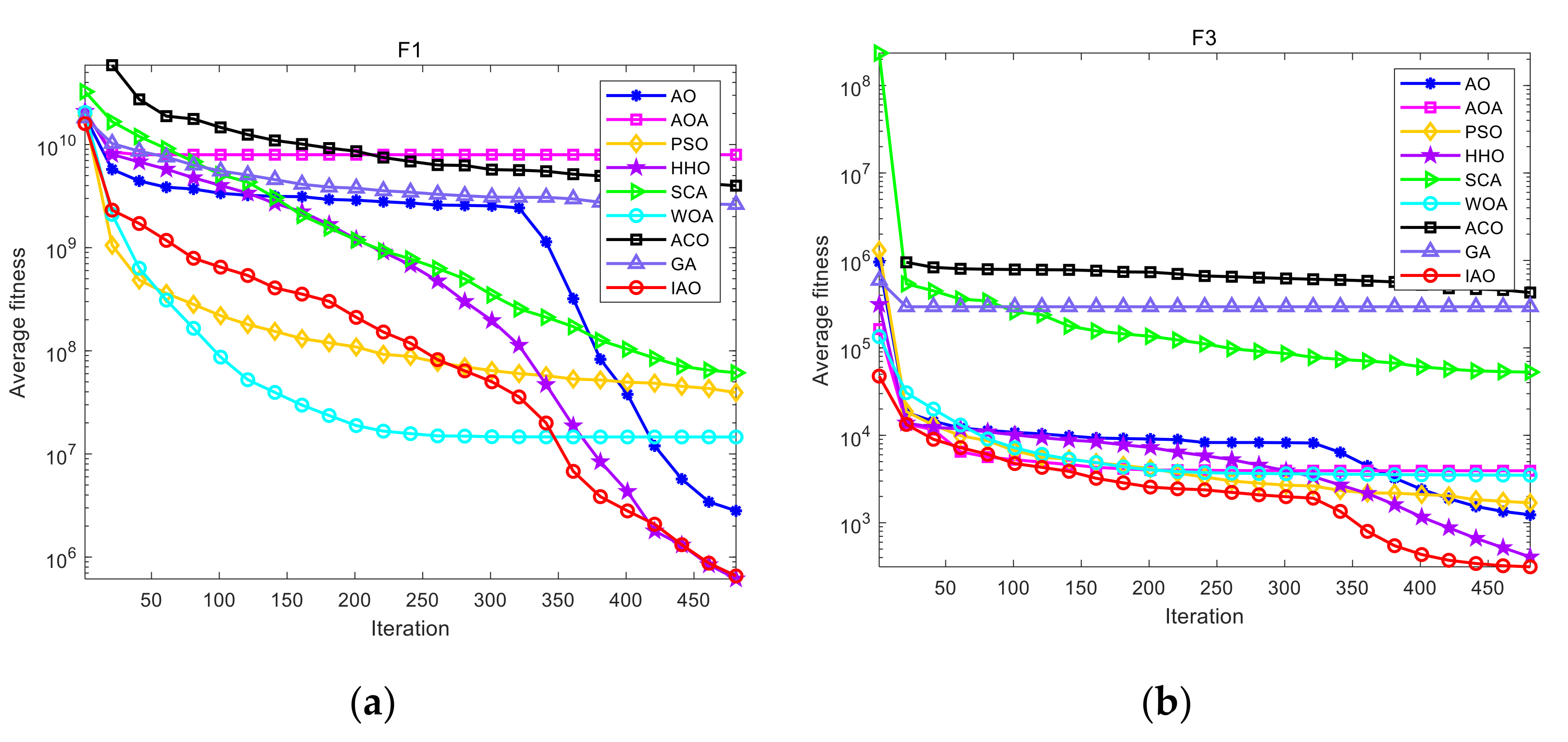
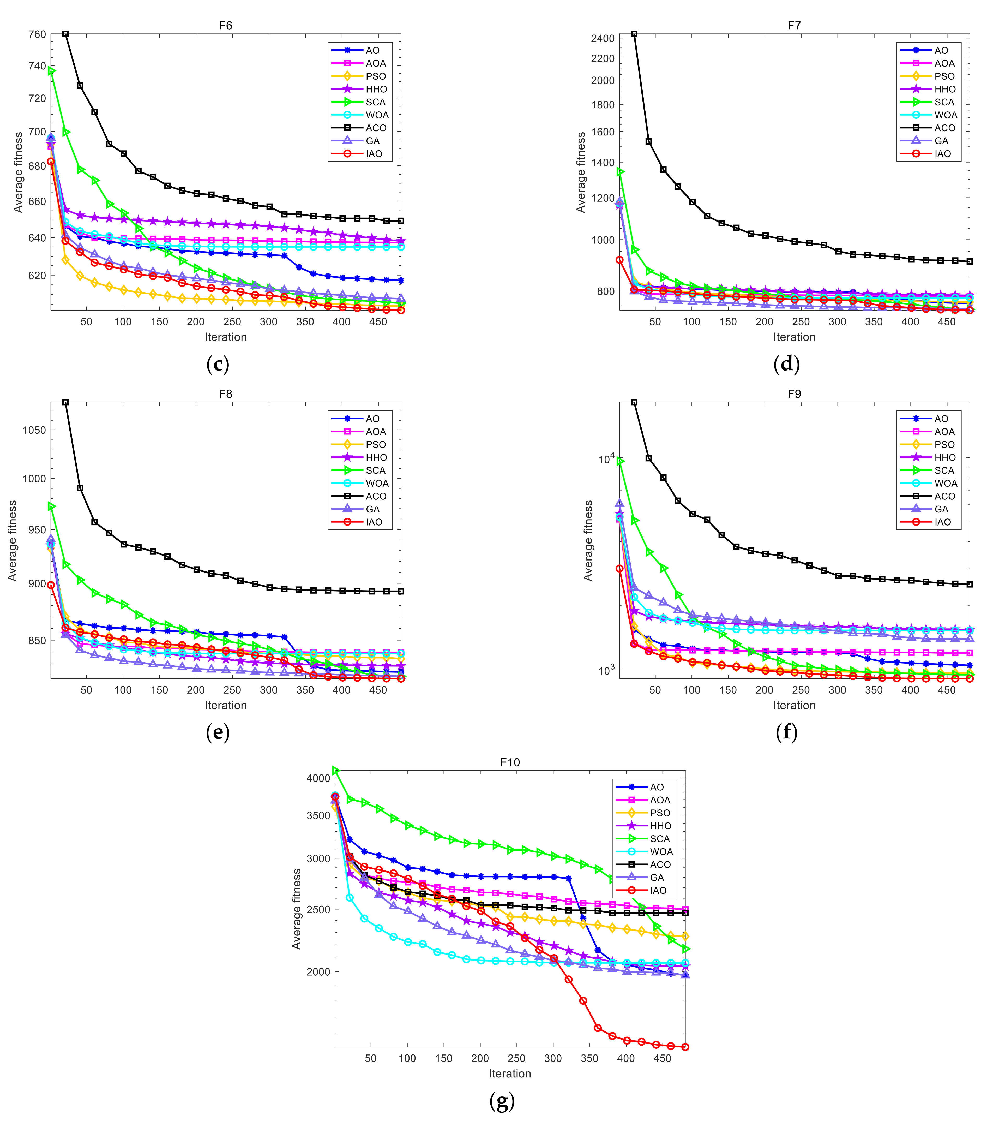
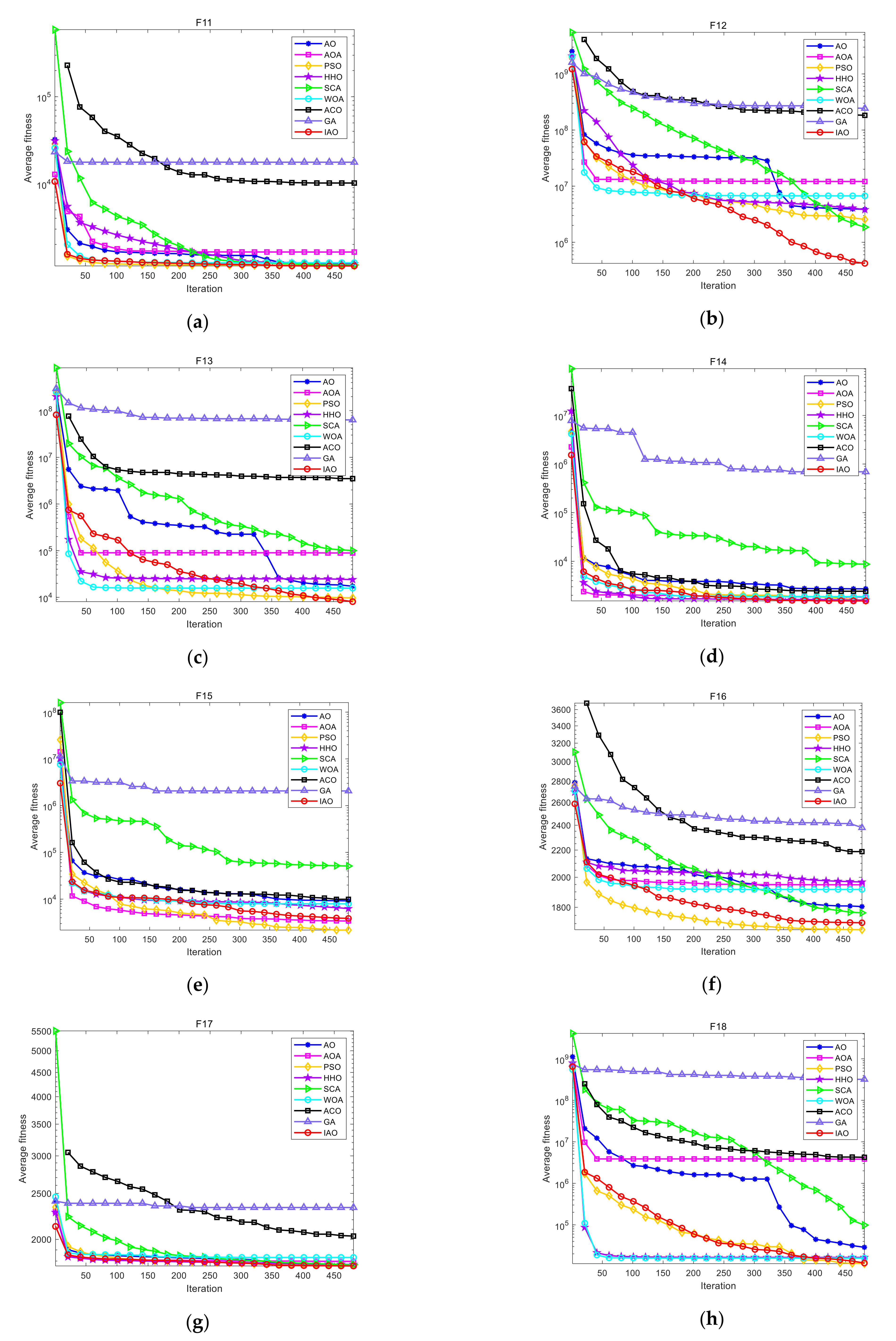
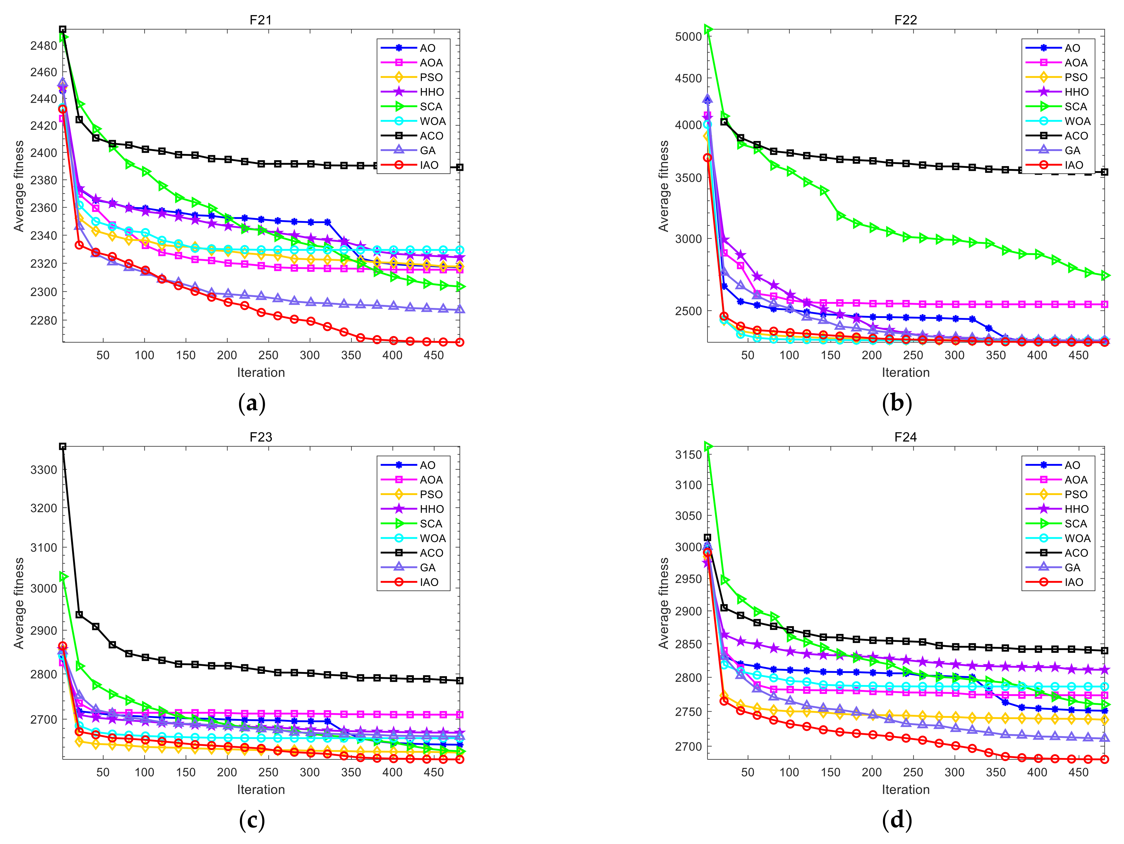
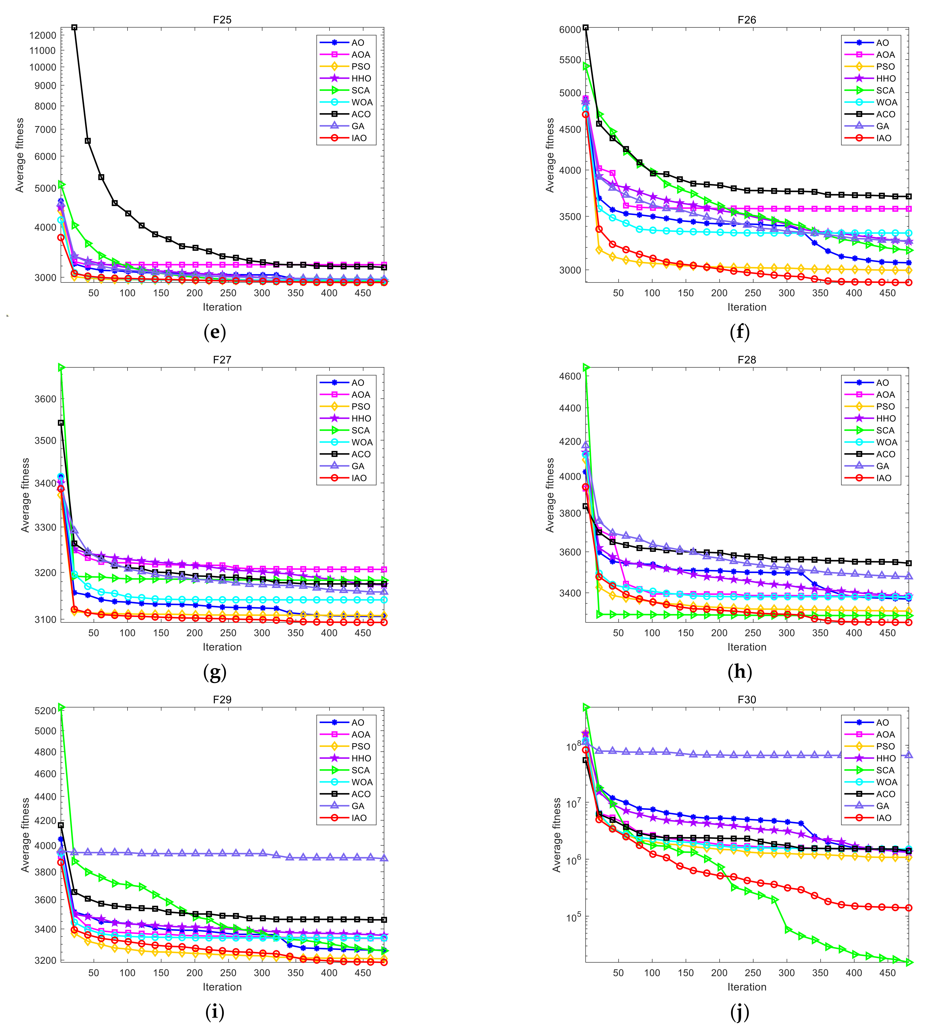
3. Comparison of Improved Aquila Optimizer with Other Algorithms

In this section, the validity of the proposed algorithm is verified by the CEC2017 test functions, which contain four types of functions: unimodal, multimodal, hybrid, and composite. The detailed description of these functions is presented in Table 1 [37], and the specific expression of the functions’ formula is shown in [38]. In order to evaluate the advantages and disadvantages of the proposed IAO, it was compared with the original Aquila Optimizer (AO) [33], Archimedes optimization algorithm (AOA) [39], particle swarm optimization (PSO) [15], Harris hawks optimization (HHO) [23], sine–cosine algorithm (SCA) [40], whale optimization algorithm (WOA) [19], ant colony optimization (ACO) [16], and Genetic algorithm (GA) [41], which are rather classical and have been widely used in practical engineering optimization problems. Related specific parameters of these algorithms were set as Table 2 shows. To obtain an unbiased experimental result, all the experiments were carried out on the same computer, the algorithms run on Windows 10(64-bit), Intel(R) Core(TM) i7-1165G7 (Santa Clara, CA, USA), CPU @2.80GHz (Santa Clara, CA, USA), MATLAB 2020a (Natick, MA, USA). In order to compare algorithms more fairly, the population size of all algorithms was 50, dimension D = 10, and the maximum number of iterations T = 500.
Table 3 shows the results of IAO and other optimization algorithms running 20 times for solving the 10-dimensional CEC2017 test set, including the best value, the mean value, the worst value, and the standard deviation. Meanwhile, according to the mean value on each function, the ranking of different algorithms was given to display the position of the IAO in all compared algorithms. As can be seen from Table 3, on the unimodal functions F1 and F3, the IAO algorithm was significantly better than other comparison algorithms, mainly because of the introduction of quasi-opposition learning strategy, which improves the solution accuracy of the algorithm. Comparing with the original population of the AO, the new initial population included more solutions closer to the optimum solution by selecting N elite individuals from the 2N individuals. That is, higher quality of the initial population ensured the accuracy of the algorithm on the unimodal functions. Thus, the IAO’s results ranked first among the nine comparison algorithms on F1 and F3.
For the multimodal functions F4–F10 with lots of local optimum, the wavelet mutation strategy was adopted to improve the ability of IAO to jump out of local optimum, which makes the algorithm more likely to find the global optimal solution. IAO ranked first on all multimodal functions, which confirmed the above hypothesis. Other traditional algorithms such as GA and ACO performed less well because of the disadvantage of falling into the local optimum easily.
For the hybrid functions F11–F20 and composite functions F21–F30, the algorithm must converge to the optimal solution in a more complex search space quickly, which is a challenge to the comprehensive performance of algorithms, and the IAO combining the quasi-opposition and wavelet mutation strategy achieved a better performance on F11–F30. Expect F15, F16, F19, and F30, the mean values of the IAO ranked first on all test functions. Overall, the IAO algorithm ranked first on 26 test functions, indicating that the IAO algorithm significantly outperformed other optimization algorithms on the CEC2017 test set. That is, by applying quasi-opposition learning and wavelet mutation strategy to the original AO algorithm, the IAO kept a better balance between exploration and exploitation, so as to improve the calculation accuracy of the original algorithm.
In the last two rows of Table 3, the average ranking and average running time are given. It can be seen that, for solving the CEC2017 test problem, the AO algorithm ranks third, and the IAO algorithm performs best. At the same time, the standard deviations of the IAO algorithm on 17 test functions were the smallest, which shows that the IAO algorithm was more stable in solving CEC2017 test functions. For the time cost, the time cost of IAO algorithm increased slightly due to the introduction of improvement strategies. The time cost of the IAO ranks seventh and the original AO ranks fifth. Thus, compared with the original AO algorithm, the slight increase in the cost of time is acceptable.
Moreover, the Wilcoxon rank-sum test was used to illustrate whether there was significant difference between the IAO and other compared algorithms. The statistical data are summarized in Table 4, where ‘−’ represents that the IAO algorithm was inferior to the comparison algorithm at the 95% significance level (α = 0.05), ‘=’ represents that there was no significant difference between the IAO algorithm and the comparison algorithm, and ‘+’ indicates that the IAO algorithm was significantly better than the comparison algorithm. According to the statistical result of the original AO algorithm 28/1/0, there was significant difference between the IAO and AO in the results on 28 test functions, which shows that the IAO algorithm had significantly improved computational accuracy compared with the original algorithm. This difference is also evident in comparison with other algorithms. According to the statistical results of the last line in Table 4, PSO had a better effect among all the comparison algorithms. It was superior to IAO in 8 test functions, but inferior to IAO in 20 test functions. Therefore, overall, IAO had a significant advantage in at least 20 test functions.
In order to compare the performance of the algorithms more intuitively, Figure 1, Figure 2, Figure 3 and Figure 4 show the average convergence curves of each algorithm on CEC2017 test functions. Due to the introduction of quasi-opposition learning strategy, the proposed IAO produced more excellent individuals in the initial population stage. Therefore, the IAO was able to close to the theoretical optimal solution with quicker speed at the beginning of the search on unimodal functions F1 and F3. PSO and WOA also showed excellent performance at the beginning, but with the increase in the number of iterations, the performance of other algorithms’ convergence speed gradually deteriorated. In functions F5, F10, F12, F13, F21, F24, F26, F28, and F30, IAO continued to search quickly and efficiently in the later stage of the search, while the convergence speed of other comparison algorithms gradually slowed down. That is, the improvement strategies in IAO overcame the defect of premature convergence which caused the terrible performance of other algorithms, especially for the traditional GA and ACO algorithms.
Therefore, the IAO algorithm may show its advantages in parameter optimization problems, combinatorial optimization problems, or path optimization and other aspects. Excellent performance in convergence speed, accuracy, and stability may help it ascertain competitiveness in practical application. Meanwhile, the convergence speed of PSO and WOA were also competitive in the early iteration stage such as F1, F18, and F19. Therefore, it would be an interesting study how to learn from the initial search methods of these two algorithms to further improve the convergence speed of IAO.

4. The Solving of China’s Rural Community Population Forecast Model Using Improved Aquila Optimizer

In recent years, with the development of population urbanization in China, and a large number of urban and rural population flows, the rural community population shows a trend of decreasing year by year. The effective prediction of China’s rural population is of great significance to the rational planning of rural construction. In this section, a mathematical model is established to forecast the rural population. Table 5, Table 6 and Table 7 show the rural population during 1990−1999, 2000−2009, and 2010−2019, respectively. In addition, when the rural population forecasting was carried out, the population of the first 25 years (1990−2014) was used to train the model, so as to obtain the specific parameter values of the model, and then the fitting effect of the model was tested with the population of the last 5 years (2015−2019). These rural community population data can be found in the “China Statistical Yearbook 2020” compiled by the National Bureau of Statistics of China. In the China Statistical Yearbook’ China’s total population can be divided into urban population and rural population according to urban and rural areas. This study was based on the prediction o’ China’s rural population.
In order to more intuitively observe the changing trend of the rural population, Figure 5 shows the bar chart of the rural population during 1990−2019. It can be seen that during 1990−1995, the rural population showed a slow growth trend, and after 1995, the rural population showed a declining trend year by year.

4.1. China’s Rural Population Forecasting Model

According to the changing trend of the rural community population, this paper used the consistent fractional accumulation nonhomogeneous grey Bernoulli model (called CFANGBM(1, 1, b, c) for short) to fit and forecast the above rural population. The model in this section is based on the consistent fractional accumulation and inverse accumulation operators.
Given the original data sequence:
X ( 0 ) = ( x ( 0 ) ( 1 ) , x ( 0 ) ( 2 ) , , x ( 0 ) ( n ) ) ,
then, its consistent r fractional order accumulative sequence is defined as:
X ( r ) = ( x ( r ) ( 1 ) , x ( r ) ( 2 ) , , x ( r ) ( n ) ) ,
where:
x ( r ) ( k ) = i = 1 k k i + [ r ] 1 k i x ( 0 ) ( i ) i [ r ] r , r R + , k = 1 , 2 , , n ,
The consistent r fractional order inverse accumulative sequence of Equation (22) is defined as:
X ( r ) = ( x ( r ) ( 1 ) , x ( r ) ( 2 ) , , x ( r ) ( n ) ) ,
where:
x ( r ) ( k ) = k [ r ] r i = 1 k ( 1 ) k i [ r ] k i x ( 0 ) ( i ) , k = 2 , 3 , , n , x ( r ) ( 1 ) = x ( 0 ) ( 1 ) .
Let the original sequence X(0) and its consistent r fractional order accumulation sequence X(r) be shown in Equations (22) and (23), respectively. Then, the CFANGBM(1, 1, b, c) is represented as the following differential equation:
d x ( r ) ( t ) d t + a x ( r ) ( t ) = ( b t + c ) ( x ( r ) ( t ) ) γ , γ R ,
which is often called the whitening equation of the CFANGBM(1, 1, b, c).
Multiply both sides of Equation (27) by ( x ( r ) ( t ) ) γ and obtain Equation (28).
d x ( r ) ( t ) d t ( x ( r ) ( t ) ) γ + a ( x ( r ) ( t ) ) 1 γ = b t + c ,
Let y ( r ) ( t ) = ( x ( r ) ( t ) ) 1 γ . Then, Equation (28) can be transformed into:
d y ( r ) ( t ) d t + ( 1 γ ) a y ( r ) ( t ) = ( 1 γ ) ( b t + c ) ,
The constant variation method is used to solve Equation (29), and y ( r ) ( t ) can be obtained:
y ( r ) ( t ) = y ( r ) ( 1 ) + b a 2 ( 1 γ ) b + c a e a ( 1 γ ) ( t 1 ) + b t + c a b a 2 ( 1 γ ) ,
Further, since y ( r ) ( t ) = ( x ( r ) ( t ) ) 1 γ , the x ( r ) ( t ) is given by:
x ( r ) ( t ) = ( x ( r ) ( 1 ) ) 1 γ + b a 2 ( 1 γ ) b + c a e a ( 1 γ ) ( t 1 ) + b t + c a b a 2 ( 1 γ ) 1 1 γ ,
From Equation (24), it can be deduced that x ( r ) ( 1 ) = x ( 0 ) ( 1 ) . Therefore, the time response function of Equation (27) is:
x ^ ( r ) ( k ) = ( x ( 0 ) ( 1 ) ) 1 γ + b a 2 ( 1 γ ) b + c a e a ( 1 γ ) ( k 1 ) + b k + c a b a 2 ( 1 γ ) 1 1 γ ,
where k = 2 , 3 , , n .
When the fractional order r is given to the model parameters a, b, c, and γ , Equation (32) can fit (kn) and forecast (k > n) the original sequence. a, b, and c are obtained by least-square estimation, and the expression is as follows:
( a , b , c ) T = ( B T B ) 1 B T Y ,
where, B and Y are as follows, respectively:
B = ( 1 γ ) z ( r ) ( 2 ) 3 2 1 z ( r ) ( 3 ) 5 2 1 z ( r ) ( n ) 2 n 1 2 1 ,   Y = y ( r ) ( 1 ) y ( r ) ( 2 ) y ( r ) ( 2 ) y ( r ) ( 3 ) y ( r ) ( n 1 ) y ( r ) ( n ) ,
where: z ( r ) ( k ) = 1 2 ( y ( r ) ( k 1 ) + y ( r ) ( k ) ) , k = 2 , 3 , , n .
Substitute y ( r ) ( t ) = ( x ( r ) ( t ) ) 1 γ into Equation (34). Then, B and Y are transformed into:
B = ( 1 γ ) 1 2 ( x ( r ) ( 1 ) ) 1 γ + ( x ( r ) ( 2 ) ) 1 γ 3 2 1 1 2 ( x ( r ) ( 2 ) ) 1 γ + ( x ( r ) ( 3 ) ) 1 γ 5 2 1 1 2 ( x ( r ) ( n 1 ) ) 1 γ + ( x ( r ) ( n ) ) 1 γ 2 n 1 2 1 ,  
Y = ( x ( r ) ( 1 ) ) 1 γ ( x ( r ) ( 2 ) ) 1 γ ( x ( r ) ( 2 ) ) 1 γ ( x ( r ) ( 3 ) ) 1 γ ( x ( r ) ( n 1 ) ) 1 γ ( x ( r ) ( n ) ) 1 γ ,
By substituting the obtained a, b, and c into Equation (32), x ^ ( r ) ( k ) , k = 1 , 2 , , n can be obtained, and the consistent fractional order inverse accumulation is performed on it. The predicted value of the CFANGBM(1, 1, b, c) model can be computed by Equation (37):
x ^ ( 0 ) ( k ) = k [ r ] r i = 1 k ( 1 ) k i [ r ] k i x ^ ( r ) ( i ) , k = 2 , 3 , , n , x ^ ( 0 ) ( 1 ) = x ^ ( r ) ( 1 ) .
It can be seen that the key to prediction by using the CFANGBM(1, 1, b, c) model is to find the optimal parameters r and γ, so this problem can be transformed into an optimization problem, and the optimization goal is to minimize the mean absolute percentage error between the predicted value and the real value. The objective function and constraint conditions of the optimization problem are:
minimize   arg ( f ( r , γ ) ) = 1 n 1 k = 2 n x ^ ( 0 ) ( k ) x ( 0 ) ( k ) x ( 0 ) ( k ) × 100 % ,
subject to:
( a , b , c ) T = ( B T B ) 1 B T Y , x ^ ( r ) ( k ) = ( x ( 0 ) ( 1 ) ) 1 γ + b a 2 ( 1 γ ) b + c a e a ( 1 γ ) ( k 1 ) + b k + c a b a 2 ( 1 γ ) 1 1 γ , x ^ ( 0 ) ( k ) = k [ r ] r i = 1 k ( 1 ) k i [ r ] k i x ^ ( r ) ( i ) , k = 2 , 3 , , n , x ^ ( 0 ) ( 1 ) = x ^ ( r ) ( 1 ) .

4.2. The Steps of Improved Aquila Optimizer Solving China’s Rural Population Forecasting Model

As the above model is nonlinear, it is difficult to solve it using conventional methods. Therefore, this study used the IAO algorithm to optimize the parameters of the above China rural population forecasting model, so as to predict China’s population data from 2015 to 2019 and calculate the model error. The detailed steps are described as follows:
Step1 Input the original rural population data X ( 0 ) = ( x ( 0 ) ( 1 ) , x ( 0 ) ( 2 ) , , x ( 0 ) ( n ) ) ;
Step2 Initialize the parameters of IAO, and initialize the individuals randomly by Equation (1);
Step3 Calculate quasi-opposition individual X q of current individual X based on Equation (17); and then take Equation (38) as the objective function, and select the N individuals with better fitness value from X X q as the current population;
Step4 When t < T, calculate the fitness value of each individual, record the best solution Xbest, and update the parameters x, y, QF, G1, and G2;
Step5 When t ( 2 / 3 ) T , perform the exploration operation of the algorithm. If the random number r a n d 0.5 , update the current solution by Equation (2); if the random number r a n d > 0.5 , update the current solution by Equation (4);
Step6 When t > ( 2 / 3 ) × T , perform the exploitation operation of the algorithm. If the random number r a n d 0.5 , update the current solution by Equation (11); if the random number r a n d > 0.5 , update the current solution by Equation (12);
Step7 When r a n d 0.5 , execute wavelet mutation by Equation (18);
Step8 Let t = t + 1. If t < T, return Step4; otherwise, output the minimum error value fit(Xbest) and the corresponding optimal parameter values r and γ.
Figure 6 shows the steps for the IAO to solve the China’s rural community population forecasting model.

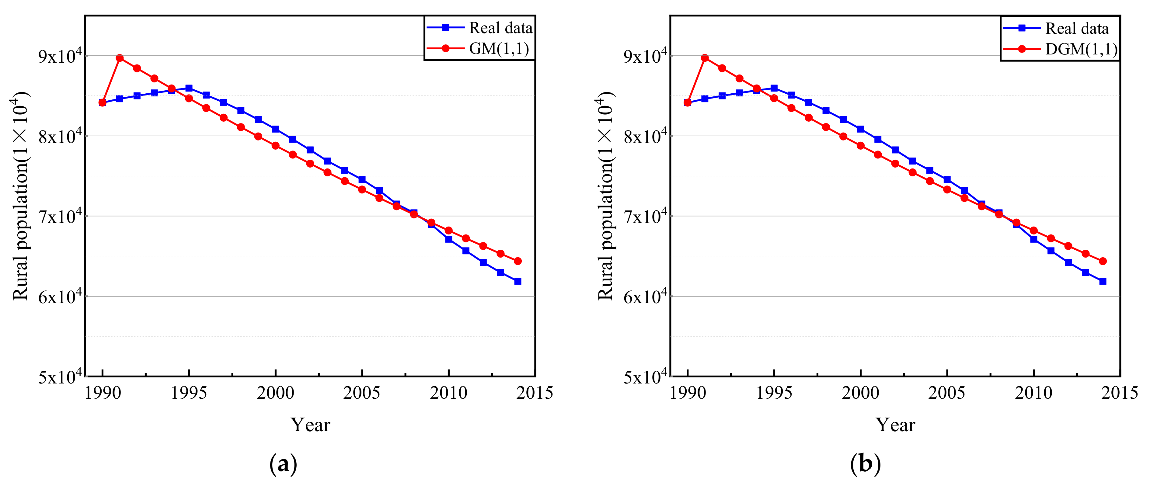
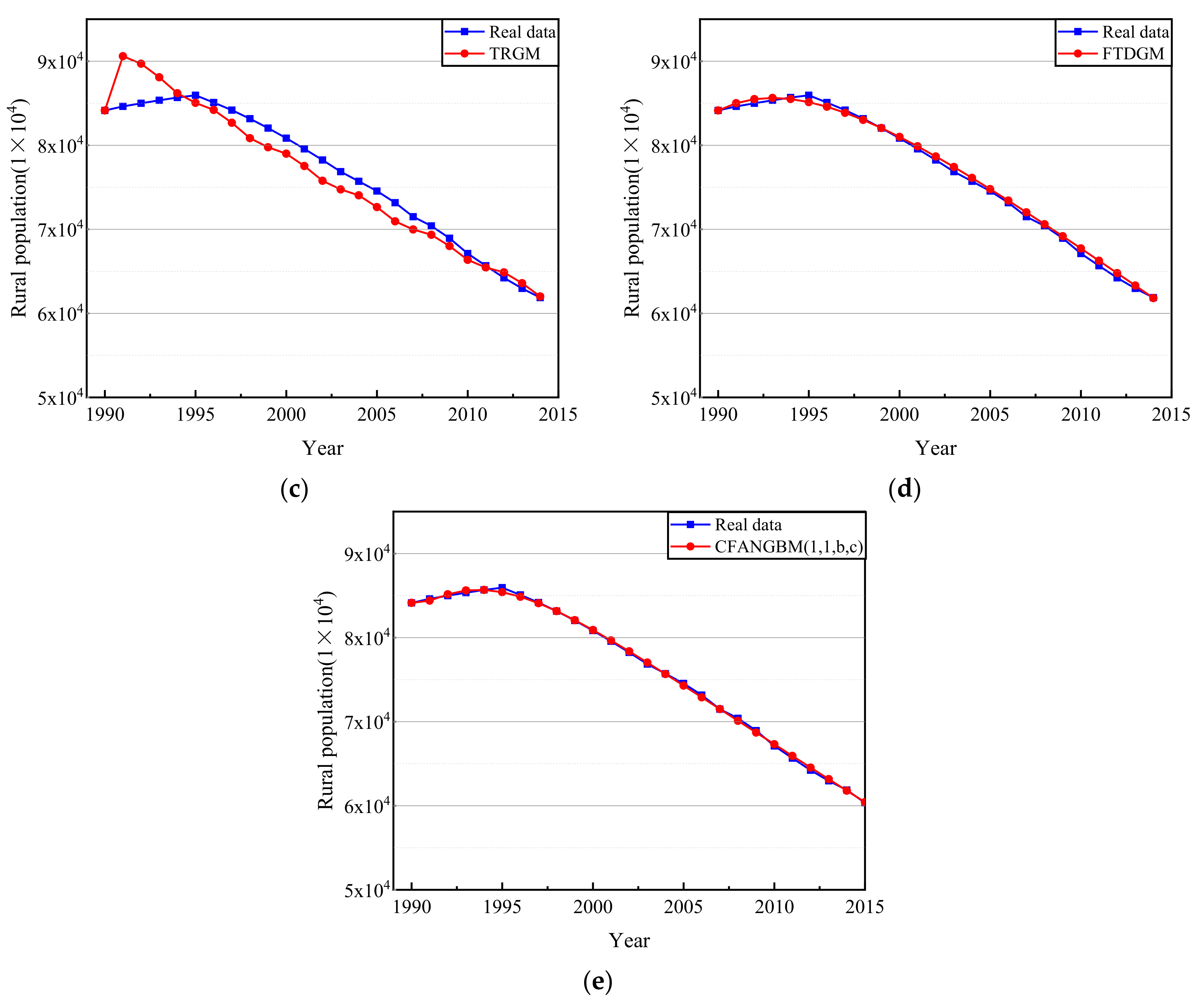
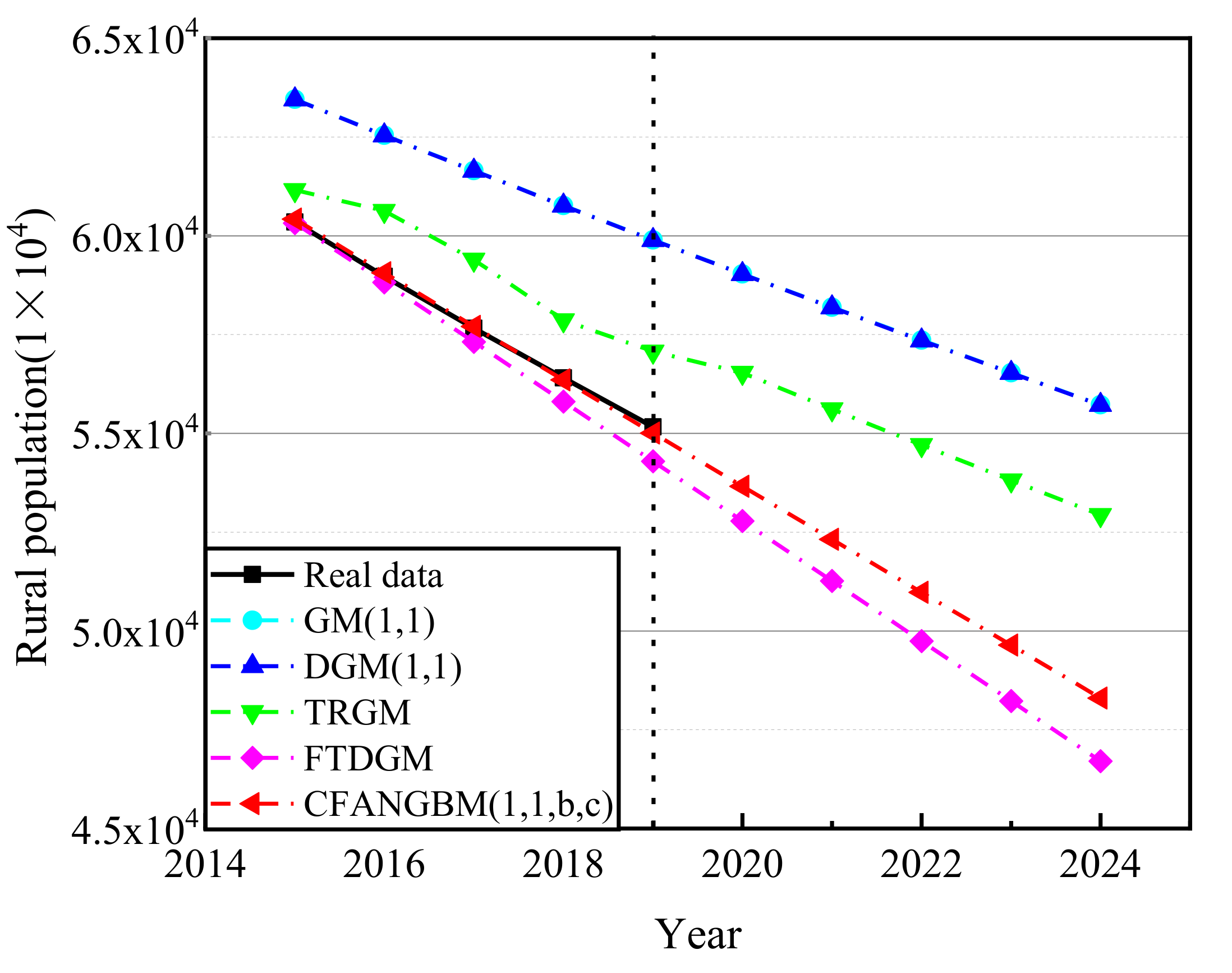
4.3. Experimental Result Analysis of China’s Rural Population Forecasting Model

In this section, the CFANGBM(1, 1, b, c) model is compared with the other four models to verify the effectiveness of the proposed model in forecasting China’s rural population. These four comparison models are GM(1, 1) [11], DGM(1, 1) [13], TRGM [12], and FTDGM [14], respectively. In order to compare the advantages and disadvantages of the five forecasting models, the evaluation criteria for the advantages and disadvantages of the models are firstly given. The specific expressions of the four evaluation criteria are shown in Table 8.
Table 9 displays the fitted China’s rural community population from 1990 to 2014 based on different models. Compared with the real data of rural population, the fitted error is given in Table 10 to measure the performance of different forecasting methods. As can be seen from Table 10, the results of the CFANGBM(1, 1, b, c) based on the IAO algorithm ranked first on all four evaluation criteria, and its fitted data of rural population in China were closest to the real data, which was better than the fitting effect of other comparison models. Among them, the predicted rural population based on GM(1, 1), DGM(1, 1), and TRGM deviated greatly from the real data.
Figure 7 shows the comparison between the predicted data of the five models and the real data, from which it can be seen that the rural population reached the maximum value in 1995, but the GM(1, 1) and DGM(1, 1) methods had a great error in fitting the data at this stage. That is, the GM(1, 1) and DGM(1, 1) models would face great challenges with data with volatility characteristics, though they are effective for monotonically increasing or decreasing data. By adding triangulation correction, the TRGM method had better performance than GM(1, 1) in the later stage. In Figure 7c, the fitted data based on TRGM are closer to the real data, especially after 2009. However, for the whole stage from 1990 to 2014, it could not obtain better results by triangulation correction. Furthermore, the FTDGM method obtains more reasonable fitted data around 1995. The fitting curve of it was closer to the real curve than GM(1, 1), DGM(1, 1), and TRGM. Finally, in Figure 7e, the fitted data obtained by the CFANGBM(1, 1, b, c) method almost coincide with the real data, which is consistent with the results in Table 10. That is, by introducing the linear correction and searching the suitable parameters by the proposed IAO, the CFANGBM(1, 1, b, c) was able to fit data with different characteristics. Especially around the turning point of the population data, the parameters could be adjusted intelligently by the IAO algorithm to accommodate rapid changes in data. Thus, the approach in this study can achieve better fitting effects for more complex data.
The best parameters could be obtained by regarding the data from 1990 to 2014 as the training data. Then, Table 11 shows China’s rural population predicted by the five prediction models from 2014 to 2019, which were compared with the real data. The forecasting errors of the five prediction models are listed in Table 12.
As can be seen from Table 11, besides the CFANGBM(1, 1, b, c) method, the other four methods had poorer performance in predicted error than fitted error. The MAPE of GM(1, 1), DGM(1, 1), and TRGM reached about 10%, which means the predicted data obtained by these methods was unreasonable. It is obvious that the CFANGBM(1, 1, b, c) method based on the IAO was effective for China’s rural population forecasting with the smallest predicted error. Next, all the fitted and predicted data were used to plot Figure 8. In the enlarged sub-figure in Figure 8, the predicted data obtained by the CFANGBM(1, 1, b, c) method were closest to the real data, while other methods deviated from the real data.
Finally, the predicted data in the next five years (2020−2024) are given in Table 13. Figure 9 is the trend line of the predicted data from 2014 to 2024 based on the different models. On the right side of the black vertical line in Figure 9 are the predicted data of China’s rural population in the next five years (2020−2024). It is obvious that the trend of the red curve most closely matched the population data from 2014 to 2019. However, the trend curves based on other models were higher or lower, which is not suitable for the future prediction. By optimizing the parameters in the CFANGBM(1, 1, b, c) model through the proposed IAO, the method can be used to data forecast with higher precision more widely.

5. Conclusions

In this study, the proposed IAO algorithm was used to optimize the parameters of the forecasting model CFANGBM(1, 1, b, c), and then to predict China’s rural population. Firstly, an improved Aquila Optimizer with higher computational accuracy and faster convergence speed was proposed. Based on the original AO algorithm, the following two strategies were introduced to improve it: (1) quasi-opposition learning strategy, which enhances population diversity and improves the quality of solution; (2) wavelet mutation strategy, which enhances the ability of the algorithm to jump out of the local optimum, and improves the calculation accuracy of the algorithm. The advantages of the proposed IAO algorithm were verified by comparison with other intelligent algorithms on CEC2017 test functions.
Secondly, the proposed IAO was applied to the CFANGBM(1, 1, b, c) model which is used to forecast the rural population in China, and the model was compared with GM(1, 1), DGM(1, 1), TRGM and FTDGM. The experimental results showed that the CFANGBM(1, 1, b, c) model had smaller fitting and prediction errors compared with the other four models, and its fitting effect and prediction results were closer to the real value. This illustrates the superiority of the CFANGBM(1, 1, b, c) model in predicting the rural population, and also verifies the effectiveness of using the IAO algorithm to solve the model parameters. In addition, the forecast data of China’s rural population from 2020 to 2024 were given.
In future work, the improved algorithm will be considered to be applied to other various applications, such as image processing, text and data mining, feature selection, task scheduling, and others. Further, the CFANGBM(1, 1, b, c) model is also likely to be used for forecast of economic growth, climate changing, and resource consumption, etc.

Supplementary Materials

Author Contributions

Conceptualization, L.M. and Y.Z.; data curation, L.M. and J.L.; formal analysis, L.M. and J.L.; funding acquisition, J.L. and Y.Z.; investigation, L.M. and J.L.; methodology, L.M., J.L. and Y.Z.; resources, L.M. and Y.Z.; software, L.M. and J.L.; supervision, J.L.; validation, L.M.; visualization, J.L. and Y.Z.; writing—original draft, L.M. and J.L.; writing—review and editing, L.M., J.L. and Y.Z. All authors have read and agreed to the published version of the manuscript.

Funding

This work was supported by the National Social Science Foundation Project Research on Cultural Landscape Protection of Ethnic Minority Traditional Villages in Western Hubei (Grant No. 19BSH097).

Institutional Review Board Statement

Not applicable.

Informed Consent Statement

Not applicable.

Data Availability Statement

All data generated or analyzed during this study were included in this published article (and its Supplementary Materials).

Conflicts of Interest

The authors declare that there is no conflict of interests regarding the publication of this paper.

References

  1. He, C.F.; Chen, T.M.; Mao, X.Y.; Zhou, Y. Economic transition, urbanization and population redistribution in China. Habitat Int. 2016, 51, 39–47. [Google Scholar] [CrossRef]
  2. Yan, J.H.; Zhu, S. Rural population transferring trend and spatial direction. China Popul. Resour. Environ. 2017, 27, 146–152. [Google Scholar]
  3. Lv, Z.; Xu, X.L.; Wan, X.R. Rural Population Prediction from the Perspective of “Rural-Urban” Dynamic Migration—Take Heilongjiang Province as an Example. J. Dalian Univ. 2019, 40, 87–95. [Google Scholar]
  4. Guan, Y.; Li, X.Y.; Zhu, J.M. Prediction and Analysis of Rural Population in China based on ARIMA Model. J. Shandong Agric. Eng. Univ. 2019, 36, 15–20. [Google Scholar]
  5. Xuan, H.Y.; Zhang, A.Q.; Yang, N.N. A Model in Chinese Population Growth Prediction. Applied Mechanics and Materials; Trans Tech Publications, Ltd.: Bäch, Switzerland, 2014; Volume 556–562, pp. 6811–6814. [Google Scholar]
  6. Zhang, Y.N.; Li, W.; Qiu, B.B.; Tan, H.Z.; Luo, Z.Y. UK population forecast using twice-pruning Chebyshev-polynomial WASD neuronet. In Proceedings of the 2016 Chinese Control and Decision Conference (CCDC), Yinchuan, China, 28–30 May 2016; pp. 3029–3034. [Google Scholar]
  7. Wang, C.Y.; Lee, S.J. Regional Population Forecast and Analysis Based on Machine Learning Strategy. Entropy 2021, 23, 656. [Google Scholar] [CrossRef]
  8. Fernandes, R.; Campos, P.; Gaio, A.R. An Agent-Based MicMac Model for Forecasting of the Portuguese Population, Portuguese Conference on Artificial Intelligence; Springer: Cham, Switzerland, 2015; pp. 702–707. [Google Scholar]
  9. Gao, H.; Yao, T.; Kang, X. Population forecast of Anhui province based on the GM (1, 1) model. Grey Syst. 2017, 7, 19–30. [Google Scholar] [CrossRef]
  10. Wei, Z. Study of Differential Equation Application in the Forecast of Population Growth. Comput. Simul. 2011, 28, 358–362. [Google Scholar]
  11. Wang, Z.X.; Li, D.D.; Zheng, H.H. Model comparison of GM (1, 1) and DGM (1, 1) based on Monte-Carlo simulation. Phys. A. 2020, 542, 123341. [Google Scholar] [CrossRef]
  12. Zhou, P.; Ang, B.W.; Poh, K.L. A trigonometric grey prediction approach to forecasting electricity demand. Energy 2006, 31, 2839–2847. [Google Scholar] [CrossRef]
  13. Xie, N.; Liu, S. Discrete grey forecasting model and its optimization. Appl. Math. Model. 2009, 33, 1173–1186. [Google Scholar] [CrossRef]
  14. Ma, X.; Mei, X.; Wu, W.Q.; Wu, X.X.; Zeng, B. A novel fractional time delayed grey model with Grey Wolf Optimizer and its applications in forecasting the natural gas and coal consumption in Chongqing China. Energy 2019, 178, 487–507. [Google Scholar] [CrossRef]
  15. Kennedy, J.; Eberhart, R.C. Particle swarm optimization. In Proceedings of the IEEE International Conference on Neural Networks, Perth, WA, Australia, 27 November–1 December 1995; pp. 1942–1948. [Google Scholar]
  16. Dorigo, M.; Birattari, M.; Stutzle, T. Ant colony optimization. IEEE Comput. Intell. Mag. 2006, 1, 28–39. [Google Scholar] [CrossRef]
  17. Yang, X.S.; Gandomi, A.H. Bat Algorithm: A Novel Approach for Global Engineering Optimization. Eng. Comput. 2012, 29, 464–483. [Google Scholar] [CrossRef] [Green Version]
  18. Mirjalili, S. Moth-flame optimization algorithm: A novel nature-inspired heuristic paradigm. Knowl.-Based Syst. 2015, 89, 228–249. [Google Scholar] [CrossRef]
  19. Mirjalili, S.; Lewis, A. The Whale Optimization Algorithm. Adv. Eng. Soft. 2016, 95, 51–67. [Google Scholar] [CrossRef]
  20. Mirjalili, S.; Mirjalili, S.M.; Lewis, A. Grey Wolf Optimizer. Adv. Eng. Soft. 2014, 69, 46–61. [Google Scholar] [CrossRef] [Green Version]
  21. Yang, X.S. Firefly Algorithm, Stochastic Test Functions and Design Optimization. Int. J. Bio-Inspir. Com. 2010, 2, 78–84. [Google Scholar] [CrossRef]
  22. Saremi, S.; Mirjalili, S.; Lewis, A. Grasshopper Optimisation Algorithm: Theory and application. Adv. Eng. Softw. 2017, 105, 30–47. [Google Scholar] [CrossRef] [Green Version]
  23. Heidari, A.; Mirjalili, S.; Farris, H.; Aljarah, I.; Mafarja, M.; Chen, H. Harris hawks optimization: Algorithm and applications. Future Gener. Comp. Syst. 2019, 97, 849–872. [Google Scholar] [CrossRef]
  24. Sulaiman, M.H.; Mustaffa, Z.; Saari, M.M.; Daniyal, H. Barnacles mating optimizer: A new bio-inspired algorithm for solving engineering optimization problems. Eng. Appl. Artif. Intell. 2020, 87, 103330. [Google Scholar] [CrossRef]
  25. Mirjalili, S.; Gandomi, A.H.; Mirjalili, S.Z.; Saremi, S.; Faris, H.; Mirjalili, S.M. Salp swarm algorithm: A bio-inspired optimizer for engineering design problems. Adv. Eng. Soft. 2017, 114, 163–191. [Google Scholar] [CrossRef]
  26. Zhao, W.G.; Zhang, Z.X.; Wang, L.Y. Manta ray foraging optimization: An effective bio-inspired optimizer for engineering applications. Eng. Appl. Artif. Intell. 2020, 87, 103300. [Google Scholar] [CrossRef]
  27. Faramarzi, A.; Heidarinejad, M.; Mirjalil, S.; Gandomi, A.H. Marine Predators Algorithm: A nature-inspired metaheuristic. Expert Syst. Appl. 2020, 152, 113377. [Google Scholar] [CrossRef]
  28. Khishe, M.; Mosavi, M.R. Chimp optimization algorithm. Expert Syst. Appl. 2020, 149, 113338. [Google Scholar] [CrossRef]
  29. Li, S.M.; Chen, H.L.; Wang, M.J.; Heidari, A.A.; Mirjalili, S. Slime mould algorithm: A new method for stochastic optimization. Future Gener. Comp. Syst. 2020, 111, 300–323. [Google Scholar] [CrossRef]
  30. Maciel, O.; Cuevas, E.; Navarro, M.A.; Zaldívar, D.; Hinojosa, S. Side-blotched lizard algorithm: A polymorphic population approach. Appl. Soft Comput. 2020, 88, 106039. [Google Scholar] [CrossRef]
  31. Abdollahzadeh, B.; Gharehchopogh, F.S.; Mirjalili, S. African vultures optimization algorithm: A new nature-inspired metaheuristic algorithm for global optimization problems. Comput. Ind. Eng. 2021, 158, 107408. [Google Scholar] [CrossRef]
  32. Abdollahzadeh, B.; Gharehchopogh, F.S.; Mirjalili, S. Artificial gorilla troops optimizer: A new nature-inspired metaheuristic algorithm for global optimization problems. Int. J. Intell. Syst. 2021, 36, 5887–5958. [Google Scholar] [CrossRef]
  33. Abualigah, L.; Yousri, D.; Elaziz, M.A.; Ewees, A.A.; Al-qaness, M.A.A.; Gandomi, A. Aquila Optimizer: A novel meta-heuristic optimization algorithm. Comput. Ind. Eng. 2021, 157, 107250. [Google Scholar] [CrossRef]
  34. Brezočnik, L.; Fister, I.; Podgorelec, V. Swarm Intelligence Algorithms for Feature Selection: A Review. Appl. Sci. 2018, 8, 1521. [Google Scholar] [CrossRef] [Green Version]
  35. Rahnamayan, S.; Tizhoosh, H.R.; Salama, M.M.A. Quasi-oppositional Differential Evolution. In Proceedings of the 2007 IEEE Congress on Evolutionary Computation, Singapore, 25 September 2021; IEEE: Singapore, 2007; pp. 2229–2236. [Google Scholar]
  36. Chatterjee, A.; Ghoshal, S.P.; Mukherjee, V. Craziness-based PSO with wavelet mutation for transient performance augmentation of thermal system connected to grid. Expert Syst Appl. 2011, 38, 7784–7794. [Google Scholar] [CrossRef]
  37. Hu, G.; Zhu, X.N.; Wei, G.; Chang, C.T. An improved marine predators algorithm for shape optimization of developable Ball surfaces. Eng. Appl. Artif. Intell. 2021, 105, 104417. [Google Scholar] [CrossRef]
  38. Awad, N.H.; Ali, M.Z.; Liang, J.J.; Qu, B.Y.; Suganthan, P.N. Problem Definitions and Evaluation Criteria for the CEC 2017 Special Session and Competition on Single Objective Real-Parameter Numerical Optimization; Nanyang Technological Univ.: Singapore, 2016. [Google Scholar]
  39. Hashim, F.A.; Hussain, K.; Houssein, E.H.; Mai, S.M.; Ai-Atabany, W. Archimedes optimization algorithm: A new metaheuristic algorithm for solving optimization problems. Appl. Intell. 2021, 51, 1531–1551. [Google Scholar] [CrossRef]
  40. Mirjalili, S. SCA: A Sine Cosine Algorithm for Solving Optimization Problems. Knowl.-Based Syst. 2016, 96, 120–133. [Google Scholar] [CrossRef]
  41. Holland, J.H. Genetic algorithms. Sci. Am. 1992, 267, 66–73. [Google Scholar] [CrossRef]
Figure 1. Convergence curves of the IAO and other algorithms on unimodal functions. (a) Convergence curve of F1, (b) Convergence curve of F3.
Fractalfract 05 00190 g001
Figure 2. Convergence curves of the IAO and other algorithms on simple multimodal functions. (a) Convergence curve of F4, (b) Convergence curve of F5, (c) Convergence curve of F6, (d) Convergence curve of F7, (e) Convergence curve of F8, (f) Convergence curve of F9, (g) Convergence curve of F10.
Fractalfract 05 00190 g002aFractalfract 05 00190 g002b
Figure 3. Convergence curves of the IAO and other algorithms on hybrid functions. (a) Convergence curve of F11, (b) Convergence curve of F12, (c) Convergence curve of F13, (d) Convergence curve of F14, (e) Convergence curve of F15, (f) Convergence curve of F16, (g) Convergence curve of F17, (h) Convergence curve of F18, (i) Convergence curve of F19, (j) Convergence curve of F20.
Fractalfract 05 00190 g003aFractalfract 05 00190 g003b
Figure 4. Convergence curves of the IAO and other algorithms on composition functions. (a) Convergence curve of F21, (b) Convergence curve of F22, (c) Convergence curve of F23, (d) Convergence curve of F24, (e) Convergence curve of F25, (f) Convergence curve of F26, (g) Convergence curve of F27, (h) Convergence curve of F28, (i) Convergence curve of F29, (j) Convergence curve of F30.
Fractalfract 05 00190 g004aFractalfract 05 00190 g004b
Figure 5. The bar chart of the rural community population during 1990−2019.
Fractalfract 05 00190 g005
Figure 6. The process of the IAO solving the China’s rural population forecasting model.
Fractalfract 05 00190 g006
Figure 7. Comparison between the predicted data and real data based on different models. (a) Fitted data based on GM(1, 1), (b) Fitted data based on DGM(1, 1), (c) Fitted data based on TRGM, (d) Fitted data based on FTDGM, (e) Fitted data based on CFANGBM(1, 1, a, b).
Fractalfract 05 00190 g007aFractalfract 05 00190 g007b
Figure 8. Comparison of the fitted data based on different models.
Fractalfract 05 00190 g008
Figure 9. Comparison of forecasting data from 2020 to 2024 based on the five models.
Fractalfract 05 00190 g009
Table 1. CEC2017 test functions.
FunctionNo.Function NameOptimal Value
Unimodal
Functions
F1Shifted and Rotated Bent Cigar Function 100
F3Shifted and Rotated Zakharov Function 300
Multimodal
Functions
F4Shifted and Rotated Rosenbrock’s Function 400
F5Shifted and Rotated Rastrigin’s Function 500
F6Shifted and Rotated Expanded Scaffer’s F6 Function 600
F7Shifted and Rotated Lunacek Bi_Rastrigin Function 700
F8Shifted and Rotated Non-Continuous Rastrigin’s Function 800
F9Shifted and Rotated Levy Function900
F10Shifted and Rotated Schwefel’s Function1000
Hybrid
Functions
F11Hybrid Function of Zakharov, Rosenbrock, and Rastrigin’s1100
F12Hybrid Function of High Conditioned Elliptic, Modified Schwefel, and Bent Cigar1200
F13Hybrid Function of Bent Cigar, Rosenbrock, and Lunacek Bi_Rastrigin1300
F14Hybrid Function of Elliptic, Ackley, Schaffer, and Rastrigin1400
F15Hybrid Function of Bent Cigar, HGBat, Rastrigin, and Rosenbrock1500
F16Hybrid Function of Expanded Schaffer, HGBat, Rosenbrock, and Modified Schwefel1600
F17Hybrid Function of Katsuura, Ackley, Expanded Griewank plus Rosenbrock, Modified Schwefel, and Rastrigin1700
F18Hybrid Function of high conditioned Elliptic, Ackley, Rastrigin, HGBat, and Discus1800
F19Hybrid Function of Bent Cigar, Rastrigin, Expanded Griewank plus Rosenbrock, Weierstrass, and expanded Schaffer1900
F20Hybrid Function of HappyCat, Katsuura, Ackley, Rastrigin, Modified Schwefel, and Schaffer2000
Composition
Functions
F21Composition Function of Rosenbrock, High Conditioned Elliptic, and Rastrigin2100
F22Composition Function of Rastrigin, Griewank, and Modified Schwefel2200
F23Composition Function of Rosenbrock, Ackley, Modified Schwefel, and Rastrigin 2300
F24Composition Function of Ackley, High Conditioned Elliptic, Griewank, and Rastrigin2400
F25Composition Function of Rastrigin, HappyCat, Ackley, Discus, and Rosenbrock2500
F26Composition Function of Expanded Scaffer, Modified Schwefel, Griewank, Rosenbrock, and Rastrigin2600
F27Composition Function of HGBat, Rastrigin, Modified Schwefel, Bent-Cigar, High Conditioned Elliptic, and Expanded Scaffer2700
F28Composition Function of Ackley, Griewank, Discus, Rosenbrock, HappyCat, and Expanded Scaffer2800
F29Composition Function of shifted and rotated Rastrigin, Expanded Scaffer, and Lunacek Bi_Rastrigin2900
F30Composition Function of shifted and rotated Rastrigin, Non-Continuous Rastrigin, and Levy Function3000
Search Range: [−100, 100]D
Table 2. The parameter settings of all comparison algorithms.
AlgorithmParameter Value
AOExploitation adjustment parameters: α 0.1, δ = 0.1
AOAConstant parameters: C1 = 2, C2 = 6, C3 = 1, C4 = 2
PSOVelocity range: 0.5 times the variable range
Cognitive and social factors: c1 = 2, c2 = 2.5
HHOThe value of E0 = [−1,1]
SCAConstant value a = 2
WOA a variable linearly decreases from 2 to 0
ACOPheromone evaporation coefficient: Rho = 0.95
Pheromones increase intensity: Q = 1
Speed of ant: Lambda = 0.5
GACrossover probability: Pc = 0.95
Mutation probability: Pm = 0.001
Select probability: Er = 0.2
IAOMutation probability is 0.5, constant s = 10,000
Table 3. Results of the comparative algorithms on CEC2017 test functions.
ResultAlgorithms
IAOAOAOAPSOHHOSCAWOAACOGA
F1Best2.05E+056.55E+053.83E+092.91E+061.48E+053.20E+062.38E+061.62E+091.43E+09
Mean4.25E+052.48E+067.97E+093.62E+075.32E+056.07E+071.46E+073.99E+092.61E+09
Worst7.26E+051.04E+071.45E+107.68E+071.52E+064.06E+088.05E+077.45E+094.46E+09
Std1.52E+052.10E+062.85E+092.03E+073.39E+051.19E+081.91E+071.58E+097.32E+08
Rank139526487
F3Best3.01E+023.26E+021.49E+035.23E+023.04E+027.66E+036.87E+021.07E+051.17E+04
Mean3.08E+021.19E+033.94E+031.64E+033.54E+025.27E+043.49E+034.17E+052.95E+05
Worst3.28E+023.05E+039.15E+032.78E+035.77E+022.03E+051.46E+041.08E+061.83E+06
Std8.61E+007.11E+021.98E+036.00E+027.12E+014.90E+044.23E+032.23E+055.91E+05
Rank136427598
F4Best4.03E+024.04E+025.81E+024.07E+024.00E+024.05E+024.06E+025.13E+025.40E+02
Mean4.05E+024.32E+027.79E+024.16E+024.19E+024.14E+024.56E+027.33E+027.67E+02
Worst4.08E+024.85E+021.10E+034.89E+024.89E+024.47E+025.78E+021.26E+031.23E+03
Std1.20E+003.46E+011.60E+021.80E+012.69E+019.81E+005.67E+011.95E+021.72E+02
Rank159342678
F5Best5.05E+025.12E+025.58E+025.22E+025.17E+025.16E+025.30E+025.63E+025.20E+02
Mean5.13E+025.31E+025.70E+025.31E+025.52E+025.27E+025.51E+025.85E+025.32E+02
Worst5.28E+025.46E+025.81E+025.44E+025.83E+025.40E+026.02E+026.04E+025.53E+02
Std6.44E+009.69E+007.18E+005.35E+001.66E+018.28E+001.81E+011.08E+017.74E+00
Rank148372695
F6Best6.00E+026.07E+026.29E+026.02E+026.14E+026.02E+026.11E+026.34E+026.02E+02
Mean6.02E+026.17E+026.37E+026.04E+026.38E+026.05E+026.35E+026.49E+026.08E+02
Worst6.06E+026.37E+026.47E+026.06E+026.60E+026.11E+026.70E+026.67E+026.19E+02
Std1.63E+007.39E+005.63E+001.26E+001.29E+012.47E+001.57E+019.59E+004.85E+00
Rank157283694
F7Best7.21E+027.34E+027.58E+027.42E+027.42E+027.26E+027.31E+028.32E+027.27E+02
Mean7.34E+027.57E+027.82E+027.62E+027.84E+027.38E+027.77E+029.05E+027.40E+02
Worst7.59E+027.86E+028.16E+027.87E+028.27E+027.55E+028.29E+029.64E+027.59E+02
Std1.15E+011.46E+011.50E+011.42E+012.55E+018.63E+002.51E+013.19E+018.44E+00
Rank147582693
F8Best8.07E+028.11E+028.26E+028.24E+028.13E+028.11E+028.17E+028.72E+028.12E+02
Mean8.18E+028.23E+028.39E+028.34E+028.28E+028.20E+028.39E+028.93E+028.20E+02
Worst8.40E+028.36E+028.50E+028.51E+028.42E+028.27E+028.70E+029.06E+028.29E+02
Std9.02E+006.83E+006.85E+007.08E+009.24E+004.72E+001.47E+018.24E+004.68E+00
Rank148652793
F9Best9.00E+029.17E+029.98E+029.12E+021.02E+039.02E+021.00E+031.80E+031.02E+03
Mean9.00E+021.03E+031.19E+039.55E+021.50E+039.39E+021.52E+032.48E+031.38E+03
Worst9.01E+021.26E+031.39E+031.04E+031.90E+031.12E+033.72E+033.53E+032.31E+03
Std2.50E-019.56E+019.51E+013.83E+012.45E+025.16E+016.03E+025.27E+023.34E+02
Rank145372896
F10Best1.24E+031.53E+031.99E+031.70E+031.48E+031.50E+031.32E+032.25E+031.55E+03
Mean1.52E+031.97E+032.50E+032.26E+032.03E+032.15E+032.06E+032.46E+031.97E+03
Worst1.82E+032.55E+032.86E+032.60E+032.46E+032.89E+032.81E+033.32E+032.52E+03
Std1.93E+022.73E+022.15E+022.60E+022.91E+023.80E+024.46E+021.28E+032.70E+02
Rank129746583
F11Best1.11E+031.13E+031.20E+031.12E+031.13E+031.12E+031.13E+033.89E+032.62E+03
Mean1.13E+031.18E+031.63E+031.14E+031.19E+031.16E+031.23E+039.97E+031.76E+04
Worst1.16E+031.34E+033.44E+031.36E+031.31E+031.33E+031.52E+032.55E+046.86E+04
Std1.50E+016.16E+015.66E+025.20E+015.18E+014.66E+019.11E+015.53E+031.48E+04
Rank147253689
F12Best1.70E+048.54E+044.25E+052.71E+058.13E+032.10E+048.48E+042.53E+072.99E+07
Mean3.92E+053.83E+061.21E+072.20E+063.53E+061.82E+066.73E+061.83E+082.37E+08
Worst2.50E+061.69E+075.72E+078.49E+061.31E+071.49E+071.92E+074.76E+084.78E+08
Std6.11E+054.42E+061.64E+072.03E+063.40E+063.67E+065.98E+061.23E+081.30E+08
Rank157342689
F13Best2.34E+033.60E+038.60E+031.69E+031.83E+035.30E+031.84E+031.69E+051.56E+06
Mean7.70E+031.69E+048.92E+049.69E+032.39E+049.98E+041.58E+043.49E+066.33E+07
Worst1.98E+044.86E+049.36E+052.78E+048.49E+042.98E+053.89E+049.28E+062.98E+08
Std4.31E+031.23E+042.09E+058.43E+031.78E+047.66E+041.19E+042.60E+066.74E+07
Rank146257389
F14Best1.47E+031.49E+031.46E+031.43E+031.47E+031.72E+031.47E+031.61E+032.40E+03
Mean1.53E+032.72E+031.85E+031.57E+031.59E+038.68E+031.88E+032.42E+036.93E+05
Worst1.75E+037.25E+035.26E+032.44E+031.90E+033.55E+042.58E+034.48E+033.17E+06
Std6.32E+011.40E+038.61E+022.27E+021.16E+028.83E+033.71E+028.62E+029.86E+05
Rank174238569
F15Best1.62E+032.06E+031.70E+031.58E+031.72E+038.67E+031.63E+033.09E+032.51E+04
Mean3.84E+039.12E+033.42E+032.16E+036.15E+035.11E+047.96E+039.81E+032.06E+06
Worst7.53E+033.43E+047.43E+033.36E+031.08E+044.04E+051.57E+042.68E+041.84E+07
Std2.02E+036.82E+031.65E+035.40E+023.23E+039.75E+043.97E+036.31E+034.07E+06
Rank362148579
F16Best1.60E+031.64E+031.73E+031.60E+031.77E+031.63E+031.65E+031.83E+032.05E+03
Mean1.70E+031.80E+031.95E+031.66E+031.96E+031.76E+031.92E+032.19E+032.37E+03
Worst1.97E+032.04E+032.17E+031.76E+032.15E+031.93E+032.22E+032.51E+032.76E+03
Std1.32E+021.19E+021.24E+026.15E+011.06E+029.19E+011.67E+021.73E+021.85E+02
Rank246173589
F17Best1.72E+031.73E+031.76E+031.73E+031.75E+031.74E+031.76E+031.88E+031.87E+03
Mean1.76E+031.77E+031.80E+031.77E+031.77E+031.77E+031.83E+032.02E+032.33E+03
Worst1.81E+031.85E+031.85E+031.86E+031.82E+031.89E+031.99E+032.25E+032.81E+03
Std2.05E+012.90E+012.42E+013.91E+012.16E+013.08E+016.87E+011.04E+022.61E+02
Rank156243789
F18Best2.88E+035.32E+033.29E+033.10E+034.27E+035.66E+032.26E+034.35E+058.26E+06
Mean1.09E+042.69E+043.83E+061.15E+041.64E+048.98E+041.58E+043.83E+063.12E+08
Worst2.29E+047.29E+044.55E+072.68E+043.76E+045.92E+053.90E+047.79E+068.05E+08
Std6.28E+031.50E+041.11E+078.09E+031.05E+041.31E+051.27E+042.11E+062.99E+08
Rank157246389
F19Best1.93E+032.13E+032.15E+031.92E+032.38E+032.04E+032.17E+031.22E+045.22E+04
Mean3.60E+032.24E+044.80E+043.00E+031.11E+042.24E+047.51E+042.44E+051.88E+07
Worst1.59E+042.22E+054.18E+059.67E+033.81E+041.43E+054.69E+051.38E+066.09E+07
Std3.14E+034.78E+049.84E+041.92E+031.06E+043.40E+041.21E+053.32E+051.88E+07
Rank246135789
F20Best2.02E+032.04E+032.09E+032.02E+032.05E+032.04E+032.07E+032.14E+032.01E+03
Mean2.04E+032.12E+032.14E+032.05E+032.17E+032.08E+032.18E+032.25E+032.06E+03
Worst2.06E+032.20E+032.24E+032.19E+032.34E+032.20E+032.34E+032.33E+032.16E+03
Std1.18E+014.80E+014.13E+014.39E+017.71E+014.46E+016.90E+015.59E+015.07E+01
Rank156274893
F21Best2.20E+032.20E+032.22E+032.20E+032.20E+032.21E+032.22E+032.37E+032.21E+03
Mean2.26E+032.32E+032.32E+032.32E+032.32E+032.30E+032.33E+032.39E+032.29E+03
Worst2.33E+032.35E+032.38E+032.34E+032.39E+032.33E+032.38E+032.40E+032.35E+03
Std5.88E+013.71E+015.62E+013.94E+016.13E+014.28E+014.92E+017.09E+005.00E+01
Rank154673892
F22Best2.30E+032.27E+032.35E+032.31E+032.31E+032.30E+032.31E+032.31E+032.31E+03
Mean2.31E+032.31E+032.54E+032.32E+032.32E+032.73E+032.32E+033.52E+032.32E+03
Worst2.31E+032.32E+032.88E+032.33E+032.33E+034.20E+032.34E+034.69E+032.34E+03
Std1.22E+001.11E+011.44E+025.09E+005.05E+006.30E+029.05E+001.81E+038.82E+00
Rank127438695
F23Best2.61E+032.62E+032.67E+032.62E+032.62E+032.62E+032.62E+032.70E+032.62E+03
Mean2.61E+032.65E+032.71E+032.63E+032.67E+032.63E+032.66E+032.78E+032.66E+03
Worst2.62E+032.67E+032.75E+032.64E+032.71E+032.66E+032.72E+032.86E+032.74E+03
Std4.33E+001.49E+012.35E+017.11E+003.01E+019.60E+002.87E+013.39E+012.89E+01
Rank148273596
F24Best2.50E+032.50E+032.59E+032.53E+032.50E+032.74E+032.56E+032.74E+032.54E+03
Mean2.68E+032.75E+032.77E+032.74E+032.81E+032.76E+032.79E+032.84E+032.71E+03
Worst2.75E+032.81E+032.89E+032.76E+032.91E+032.78E+032.83E+032.87E+032.83E+03
Std1.07E+028.65E+018.92E+016.78E+018.02E+011.03E+015.67E+012.59E+011.13E+02
Rank146385792
F25Best2.90E+032.90E+033.06E+032.90E+032.90E+032.91E+032.90E+033.00E+032.92E+03
Mean2.91E+032.93E+033.22E+032.94E+032.94E+032.93E+032.95E+033.17E+032.96E+03
Worst2.94E+032.96E+033.43E+032.95E+033.03E+032.95E+033.03E+033.30E+033.03E+03
Std2.12E+012.28E+011.03E+021.98E+012.95E+011.09E+013.13E+017.29E+012.34E+01
Rank139452687
F26Best2.82E+032.62E+033.27E+032.92E+032.82E+032.84E+032.96E+033.33E+032.87E+03
Mean2.89E+033.06E+033.58E+033.00E+033.25E+033.17E+033.34E+033.70E+033.25E+03
Worst2.95E+033.75E+033.93E+034.13E+034.15E+033.47E+034.46E+034.09E+034.11E+03
Std3.13E+012.16E+021.93E+022.66E+023.68E+021.76E+024.36E+021.81E+023.19E+02
Rank138254796
F27Best3.09E+033.09E+033.14E+033.10E+033.10E+033.08E+033.10E+033.15E+033.11E+03
Mean3.09E+033.11E+033.21E+033.11E+033.17E+033.18E+033.14E+033.18E+033.16E+03
Worst3.10E+033.12E+033.32E+033.17E+033.27E+033.20E+033.22E+033.21E+033.23E+03
Std2.37E+007.78E+003.54E+011.50E+014.08E+013.92E+014.37E+011.73E+013.24E+01
Rank129368475
F28Best3.10E+033.10E+033.28E+033.13E+033.10E+033.27E+033.18E+033.47E+033.12E+03
Mean3.26E+033.37E+033.39E+033.31E+033.38E+033.29E+033.38E+033.54E+033.48E+03
Worst3.41E+033.48E+033.77E+033.45E+033.75E+033.30E+033.74E+033.63E+033.72E+03
Std1.50E+021.18E+021.74E+021.34E+021.79E+029.88E+001.37E+024.45E+012.02E+02
Rank147352698
F29Best3.15E+033.18E+033.26E+033.17E+033.24E+033.15E+033.22E+033.35E+033.55E+03
Mean3.18E+033.26E+033.34E+033.21E+033.35E+033.26E+033.34E+033.46E+033.90E+03
Worst3.24E+033.38E+033.49E+033.35E+033.52E+033.36E+033.53E+033.56E+034.36E+03
Std2.17E+015.39E+015.67E+014.11E+017.74E+014.75E+018.17E+016.86E+012.06E+02
Rank145273689
F30Best6.82E+034.65E+031.12E+042.56E+047.54E+033.26E+031.67E+044.94E+051.19E+07
Mean1.37E+051.37E+061.46E+061.07E+061.28E+061.53E+041.51E+061.39E+066.63E+07
Worst1.45E+063.66E+064.30E+062.95E+065.13E+067.42E+047.17E+062.20E+061.42E+08
Std3.59E+051.28E+061.19E+061.14E+061.48E+061.77E+041.81E+065.67E+053.75E+07
Rank257341869
Mean Rank1.17244.1034 6.7241 3.0345 5.1724 4.1379 5.8966 8.2069 6.5517
Runtime(s)0.4300 0.2980 0.1404 0.05510.3092 0.0848 0.1146 1.3843 15.2474
Table 4. Wilcoxon rank-sum test p-values of comparison algorithms.
AOAOAPSOHHOSCAWOAACOGA
F19.17E-08/+6.80E-08/+6.80E-08/+4.25E-01/=6.80E-08/+6.80E-08/+6.80E-08/+6.80E-08/+
F39.17E-08/+6.80E-08/+6.80E-08/+9.28E-05/+6.80E-08/+6.80E-08/+6.80E-08/+6.80E-08/+
F48.36E-04/+6.80E-08/+9.17E-08/+6.01E-02/=9.13E-07/+1.20E-06/+6.80E-08/+6.80E-08/+
F53.07E-06/+6.80E-08/+2.22E-07/+1.66E-07/+1.41E-05/+6.80E-08/+6.80E-08/+2.56E-07/+
F66.80E-08/+6.80E-08/+4.68E-05/+6.80E-08/+1.41E-05/+6.80E-08/+6.80E-08/+2.69E-06/+
F71.41E-05/+7.90E-08/+1.80E-06/+3.94E-07/+1.26E-01/=2.06E-06/+6.80E-08/+3.85E-02/+
F81.33E-02/+1.20E-06/+8.60E-06/+2.34E-03/+1.26E-01/=1.81E-05/+6.80E-08/+1.14E-01/=
F96.80E-08/+6.80E-08/+6.80E-08/+6.80E-08/+6.80E-08/+6.80E-08/+6.80E-08/+6.80E-08/+
F101.60E-05/+6.80E-08/+2.22E-07/+2.69E-06/+1.80E-06/+1.29E-04/+1.22E-03/+3.50E-06/+
F112.75E-04/+6.80E-08/+5.79E-01/=1.10E-05/+3.34E-03/+2.06E-06/+6.80E-08/+6.80E-08/+
F125.87E-06/+2.96E-07/+1.25E-05/+7.41E-05/+2.75E-02/+2.69E-06/+6.80E-08/+6.80E-08/+
F131.78E-03/+3.07E-06/+7.76E-01/=7.41E-05/+3.50E-06/+6.79E-02/=6.80E-08/+6.80E-08/+
F141.20E-06/+1.48E-01/=1.64E-01/=4.39E-02/+7.90E-08/+2.47E-04/+1.92E-07/+6.80E-08/+
F151.44E-04/+7.56E-01/=9.05E-03/−2.23E-02/+6.80E-08/+3.75E-04/+9.28E-05/+6.80E-08/+
F164.70E-03/+4.68E-05/+3.51E-01/=4.54E-06/+1.33E-02/+1.29E-04/+1.92E-07/+6.80E-08/+
F172.85E-01/=3.99E-06/+8.60E-01/=9.62E-02/=2.18E-01/=2.36E-06/+6.80E-08/+6.80E-08/+
F185.90E-05/+3.85E-02/+9.46E-01/=8.59E-02/=9.75E-06/+5.25E-01/=6.80E-08/+6.80E-08/+
F194.68E-05/+9.28E-05/+2.62E-01/=8.36E-04/+5.25E-05/+2.36E-06/+7.90E-08/+6.80E-08/+
F202.06E-06/+6.80E-08/+8.82E-01/=2.96E-07/+1.79E-04/+6.80E-08/+6.80E-08/+8.60E-01/=
F216.04E-03/+1.04E-04/+6.87E-04/+7.41E-05/+8.36E-04/+1.67E-02/+8.35E-04/+2.56E-03/+
F222.00E-04/+6.80E-08/+6.80E-08/+6.92E-07/+4.60E-04/+1.06E-07/+1.22E-03/+1.38E-06/+
F231.66E-07/+6.80E-08/+5.23E-07/+6.80E-08/+2.22E-07/+1.92E-07/+6.80E-08/+1.43E-07/+
F241.41E-05/+2.75E-02/+6.67E-06/+6.92E-07/+6.01E-07/+6.01E-07/+1.23E-07/+3.15E-02/+
F255.90E-05/+6.80E-08/+2.04E-05/+4.68E-05/+3.34E-03/+4.54E-06/+6.80E-08/+9.13E-07/+
F268.29E-05/+6.80E-08/+6.92E-07/+2.04E-05/+9.13E-07/+6.80E-08/+6.80E-08/+9.13E-07/+
F276.92E-07/+6.80E-08/+6.80E-08/+6.80E-08/+4.54E-06/+6.80E-08/+6.80E-08/+6.80E-08/+
F281.12E-03/+2.85E-01/=4.11E-02/+2.94E-02/+1.00E+00/=3.97E-03/+6.80E-08/+2.75E-04/+
F296.67E-06/+6.80E-08/+3.15E-02/+7.90E-08/+3.07E-06/+7.90E-08/+6.80E-08/+6.80E-08/+
F308.29E-05/+1.10E-05/+5.17E-06/+1.81E-05/+2.80E-03/+5.17E-06/+5.23E-07/+6.80E-08/+
+/=/−28/1/026/3/020/8/125/4/025/4/027/2/029/0/027/2/0
Table 5. The rural community population in China from 1990 to 1999.
Year1990199119921993199419951996199719981999
Rural population
(×104)
84,13884,62084,99685,34485,68185,94785,08584,17783,15382,038
Table 6. The rural community population in China from 2000 to 2009.
Year2000200120022003200420052006200720082009
Rural population
(×104)
80,83779,56378,24176,85175,70574,54473,16071,49670,39968,938
Table 7. The rural community population in China from 2010 to 2019.
Year2010201120122013201420152016201720182019
Rural population
(×104)
67,11365,65664,22262,96161,86660,34658,97357,66156,40155,162
Table 8. The four evaluation criteria of the models.
ErrorAbbreviationConcrete Expression
Mean Absolute Percentage ErrorMAPE 1 n 1 k = 1 n x ^ ( 0 ) ( k ) x ( 0 ) ( k ) x ( 0 ) ( k ) × 100 %
Root Mean Square Percentage ErrorRMSPE 1 n k = 1 n x ^ ( 0 ) ( k ) x ( 0 ) ( k ) x ( 0 ) ( k ) 2 × 100 %
Mean Square ErrorMSE 1 n k = 1 n ( x ^ ( 0 ) ( k ) x ( 0 ) ( k ) ) 2
Mean Absolute Error MAE 1 n k = 1 n x ^ ( 0 ) ( k ) x ( 0 ) ( k )
Table 9. The fitted China’s rural population based on different models (×104).
YearReal DataGM(1, 1)DGM(1, 1)TRGMFTDGMCFANGBM
(1, 1, b, c)
199084,13884,138.084,138.084,138.0 84,138.0 84,138.0
199184,62089,704.789,712.590,599.5 85009.1 84,405.9
199284,99688,419.988,427.089,696.5 85,484.0 85,157.3
199385,34487,153.587,159.888,090.9 85,628.4 85,609.5
199485,68185,905.285,910.886,194.6 85,496.6 85,681.0
199585,94784,674.884,679.885,037.3 85,134.4 85,411.9
199685,08583,462.083,466.384,206.5 84,579.8 84,863.5
199784,17782,266.682,270.282,671.9 83,864.6 84,094.0
199883,15381,088.381,091.380,845.7 83,015.3 83,153.1
199982,03879,926.979,929.379,757.5 82,054.0 82,081.1
200080,83778,782.178,783.978,994.7 80,999.3 80,910.3
200179,56377,653.777,655.077,527.3 79,866.5 79,666.1
200278,24176,541.576,542.275,767.2 78,668.7 78,368.2
200376,85175,445.275,445.374,744.1 77,416.4 77,032.0
200475,70574,364.674,364.274,045.6 76,118.7 75,669.4
200574,54473,299.573,298.672,641.5 74,783.2 74,289.4
200673,16072,249.672,248.270,943.8 73,416.0 72,898.8
200771,49671,214.871,212.969,982.3 72,022.3 71,502.8
200870,39970,194.870,192.569,344.5 70,606.7 70,105.1
200968,93869,189.469,186.668,000.1 69,172.6 68,708.6
201067,11368,198.468,195.266,361.4 67,723.1 67,315.0
201165,65667,221.667,217.965,458.0 66,260.8 65,925.7
201264,22266,258.866,254.764,877.3 64,787.8 64,541.6
201362,96165,309.865,305.363,589.4 63,305.9 63,162.9
201461,86664,374.464,369.562,006.3 61,816.5 61,790.0
Table 10. The comparison of fitting errors of five forecasting models.
ErrorGM(1, 1)DGM(1, 1)TRGMFTDGMCFANGBM
(1, 1, b, c)
MAE1.6148E+071.3233E+071.6143E+073.4565E+061.6636E+06
MAPE(%)2.1986261.7386192.1977250.4779280.231867
MSE3.7681E+142.6103E+143.7681E+141.6026E+134.3480E+12
RMSPE(%)2.5100642.0017812.5093590.5352740.277700
Table 11. The predicted China’s rural population based on different models (×104).
YearReal DataGM(1, 1)DGM(1, 1)TRGMFTDGMCFANGBM
(1, 1, b, c)
201560,34663,452.463,447.161,157.760,320.960,422.7
201658,97362,543.562,537.960,631.158,820.059,060.7
201757,66161,647.761,641.759,396.557,314.857,703.8
201856,40160,764.860,758.457,865.955,806.056,351.4
201955,16259,894.459,887.857,069.054,294.255,003.1
Table 12. The comparison of forecasting errors of five forecasting models.
ErrorGM(1, 1)DGM(1, 1)TRGMFTDGMCFANGBM
(1, 1, b, c)
MAE3.9520E+075.5452E+073.9460E+073.9743E+068.3145E+05
MAPE(%)8.60810510.3038988.5950820.8824130.181523
MSE1.5946E+153.2963E+151.5898E+152.5021E+138.6257E+11
RMSPE(%)6.9917629.7551376.9812940.8963810.164034
Table 13. The predicted data from 2020 to 2024 based on different models (×104).
YearGM(1, 1)DGM(1, 1)TRGMFTDGMCFANGBM
(1, 1, b, c)
202059,036.6 59,029.6 56,532.6 52,779.8 53,658.2
202158,191.0 58,183.7 55,611.3 51,263.3 52,316.1
202257,357.6 57,349.9 54,705.0 49,745.1 50,976.3
202356,536.0 56,528.1 53,813.4 48,225.4 49,638.1
202455,726.3 55,718.1 52,936.4 46,704.4 48,300.7
Publisher’s Note: MDPI stays neutral with regard to jurisdictional claims in published maps and institutional affiliations.

