Article

A Variety of New Traveling Wave Packets and Conservation Laws to the Nonlinear Low-Pass Electrical Transmission Lines via Lie Analysis

by
Muhammad Bilal Riaz
1,2,*,
Jan Awrejcewicz
1,
Adil Jhangeer
3 and
Muhammad Junaid-U-Rehman
4
1
Department of Automation, Biomechanics and Mechatronics, Lodz University of Technology, 1/15 Stefanowskiego St., 90-924 Lodz, Poland
2
Department of Mathematics, University of Management and Technology, Lahore 54770, Pakistan
3
Department of Mathematics, Namal University, Talagang Road, Mianwali 42250, Pakistan
4
Department of Mathematics, Quaid-I-Azam University 45320, Islamabad 44000, Pakistan
*
Author to whom correspondence should be addressed.
Fractal Fract. 2021, 5(4), 170; https://doi.org/10.3390/fractalfract5040170
Submission received: 9 September 2021 / Revised: 11 October 2021 / Accepted: 11 October 2021 / Published: 18 October 2021
(This article belongs to the Special Issue Recent Advances in Computational Physics with Fractional Application)

Abstract

:
This research is based on computing the new wave packets and conserved quantities to the nonlinear low-pass electrical transmission lines (NLETLs) via the group-theoretic method. By using the group-theoretic technique, we analyse the NLETLs and compute infinitesimal generators. The resulting equations concede two-dimensional Lie algebra. Then, we have to find the commutation relation of the entire vector field and observe that the obtained generators make an abelian algebra. The optimal system is computed by using the entire vector field and using the concept of abelian algebra. With the help of an optimal system, NLETLs convert into nonlinear ODE. The modified Khater method (MKM) is used to find the wave packets by using the resulting ODEs for a supposed model. To represent the physical importance of the considered model, some 3 D , 2 D , and density diagrams of acquired results are plotted by using Mathematica under the suitable choice of involving parameter values. Furthermore, all derived results were verified by putting them back into the assumed equation with the aid of Maple software. Further, the conservation laws of NLETLs are computed by the multiplier method.

1. Introduction

The nonlinear evolution equations (NLEEs) explain the physical problems in different branches of engineering and nonlinear science, for example, plasma physics, biology, fluid mechanics, optics, solid-state physics, etc. [1,2]. Numerical and analytical solutions of NLEEs play a significant role in understanding the nonlinear physical models that are appearing in nonlinear sciences as well as many other branches of science, including natural sciences. Furthermore, the effort in computing the exact travelling wave patterns of NLEEs through different methods has developed speedily in the last few years, which is one of the important and advanced subjects of nonlinear science, engineering, and theoretical physics. Subsequently, we know the hypothesis of the exceptional waves in a particular soliton. Solitons have an important role in several physical phenomena and they show up in different shapes, for example, kink, bright breather, pulse, dark, envelope, and many others.
Many numbers of significant techniques for the analytical and stable soliton and wave patterns of physical models have presently been created with the help of Matlab, Mathematica, etc., such as the differential transformation technique [3], the modified exponential-function [4] method, the ( G / G ) -expansion [5] technique, the improved ( G / G ) -expansion [6] technique, the rational ( G / G ) [7] technique, the generalized Kudryashov [8] method, the homotopy analysis [9] scheme, the mean finite difference Monte-Carlo [10] technique, the Hirota’s bilinear technique [11], the approach of modified simple [12] equation, the F-expansion [13] technique, the Exp-function [14] scheme, the sine-Gordon expansion [15] scheme, the modified Kudryashov [16] method, the extended trial Equation [17] scheme, the improved tan ( Ψ ( η ) / 2 ) -expansion [18] scheme, the first integral [19] technique, the Adomian decomposition [20] method, the exponential rational function [21] technique, the rational function [22] technique, the unified scheme [23], the generalized projective Riccati [24] scheme, the multi-symplectic Runge-Kutta [25] technique, the modified extended tanh [26] scheme, the generalized unified technique [27], the modified auxiliary [28] technique, and other many methods and details are described in [29,30,31,32,33,34,35,36,37,38,39,40,41,42,43,44,45].
Many kinds of solutions are computed by using different analytical schemes such as e homogeneous balance technique, the auxiliary equation technique and the Jacobi elliptic expansion scheme, and many other techniques which are described and cited here. In this research, we are using the MKM, which has not been used previously for this model. Using this useful method on our supposed equation, we find some new kinds of wave patterns which are fruitful and very interesting results. We have used a MKM to get the required results and we obtain bright solutions, soliton-like solutions, singular bright solutions, periodic soliton solutions, and combined soliton solutions. These results are in the form of trigonometric and hyperbolic functions. There are different kinds of solutions for low pass electrical transmission lines that are computed in [46,47,48,49,50] and many other related data of this model can be seen in the literature which is cited in this article. As far as we know, the outcomes represented in this paper generally have not been described in the literature. The solutions we have developed here are new and very useful in the different branches of science.
Lie method [51,52,53,54] is employed to analyse the NLETLs. We have to construct the classical symmetries of the assumed model. We see that the obtained vector field forms an abelian algebra. We find some new travelling wave results for the NLETLs by utilizing an optimal system of Lie symmetry vectors by using the concept of abelian algebra. With the help of an optimal system, NLETLs convert into nonlinear ODE. Using the theory of the Lie symmetry method [55,56,57], we get the various forms of significant results to the assumed PDE. Then, we explore the wave solutions with the help of the integration technique, namely the modified Khater method [58,59], to solve the NLPDEs depicting the wave proliferation in the NLETLs. By using the translational vectors and their linear combinations, the NLETLs are converted to an equation wave proliferation in ordinary differential equation NLETLs. MKM is employed to find some new trigonometric and hyperbolic results which represent the consistency by Maple. To represent the physical importance of the considered model, some 3 D , 2 D , and density diagrams of the acquired results are plotted by using Mathematica under the suitable choice of involving parameters values. Furthermore, all derived results were verified by putting them back into the assumed equation with the aid of Maple software. Further, the conservation laws of NLPETLs are computed by the multiplier method. In recent years, many scientists have developed the use of the Lie theory, including Ibragimov [60], Olver [61], A.F Cheviakov [62] and Bluman [63].
In this article, we will discuss the nonlinear low-pass electrical transmission line (NLPETL) Equation [64,65] of the following form:
U τ τ l 1 ( U 2 ) τ τ + l 2 ( U 3 ) τ τ δ 2 U θ θ δ 4 12 U θ θ θ θ = 0 ,
where U = U ( θ , τ ) is the voltage and l 1 , l 2 , δ are the constants. Spatial component θ and temporal component τ represent the proliferation distance and slow time, respectively. The actual parts of the derivation of Equation (1) applying Kirchhoff’s laws are presented in [47], which are precluded here for brevity. The travelling wave and soliton solutions of Equation (1) are derived in [48]. The expansion method for describing given model and the generalized projective Riccati equations method and its applications to non-linear PDEs describing the given equation are in [49,50].
The investigation of NLETLs and their care arrangements are significant for different applied fields, for example, interfacing radio transmitters and collectors with their receiving wires, appropriating satellite TV signals, trunk lines directing calls between phone exchanging focuses, PC network associations, and rapid PC information transports. Furthermore, in interchanges and electronic designing, a transmission line is a specific medium or other construction intended to convey exchanging current of radio recurrence. NLTLs are additionally given a valuable method to check how the nonlinear excitations act inside the medium and to show the colourful properties of new frameworks [66].
Conservation laws play a very important role in constructing the analytical results of different types of nonlinear physical models. Furthermore, conservation laws are used for the reduction of PDEs, to construct the numerical, analytical, and solitary wave results. Various methods are developed to find the conservation laws, including Naz et al. [67], Herman et al. [68] and A.F. Cheviakov [69], who constructed the package GeM on Maple to find the conservation laws for PDEs. Here, we are using the multiplier scheme [70] to find the conservation laws for the assumed model. To the best of our knowledge, the supposed equation is not described by the MKM and no one has computed the conservation laws of this physical model. The pattern of this paper is as follows, in Section 2, preliminaries are presented. Classical symmetries are computed in Section 3. The optimal system, wave patterns, and graphical diagrams are described in Section 4. Conservation laws of the NLETLs are constructed in Section 5. At the end of this article, the conclusion is stated.

2. Preliminaries

2.1. Modified Khater Method

We describe the modified Khater method [71,72] to construct a new wave pattern for a supposed model. In this regard, some details of this method are given below;
(Step 1): Suppose a general nth order PDE:
H ( U , U θ , U θ θ , . . . , U τ , U τ τ , . . . ) = 0 ,
where U = U ( θ , τ ) is unknown and H is a polynomial function w.r.t specified variables.
(Step 2): Introducing the wave transformation
ϱ = τ a θ , U ( θ , τ ) = Q ( ϱ ) ,
using above transformation (3) to convert the partial differential Equation (2) into ordinary differential equation below:
F ( Q , Q , Q , . . . ) = 0 .
(Step 3): It is assumed that the general solution of nonlinear ODE (4) can be written as:
Q ( ϱ ) = j = 0 m k j B j ( ϱ ) ,
where k j ( 0 < j n ) are the arbitrary constants and B ( ϱ ) is the solution of the equation:
B ( ϱ ) = l n ( ϑ ) ( γ 1 + γ 2 B ( ϱ ) + γ 3 B 2 ( ϱ ) ) ,
where ϑ 0 , 1 and γ 1 , γ 2 , and γ 3 are the constants.
After assuming Δ = γ 2 2 4 γ 3 γ 1 , the solutions of Equation (6) represented as:
1: If Δ < 0 and γ 3 0 , then
B 1 ( ϱ ) = γ 2 2 γ 3 + Δ 2 γ 3 tan ϑ ( Δ 2 ϱ ) , B 2 ( ϱ ) = γ 2 2 γ 3 Δ 2 γ 3 cot ϑ ( Δ 2 ϱ ) , B 3 ( ϱ ) = γ 2 2 γ 3 + Δ 2 γ 3 ( tan ϑ ( Δ ϱ ) ± r s sec ϑ ( Δ ϱ ) ) , B 4 ( ϱ ) = γ 2 2 γ 3 Δ 2 γ 3 ( cot ϑ ( Δ ϱ ) ± r s csc ϑ ( Δ ϱ ) ) , B 5 ( ϱ ) = γ 2 2 γ 3 + Δ 4 γ 3 ( tan ϑ ( Δ 4 ϱ ) cot ϑ ( Δ 4 ϱ ) ) .
2: If Δ > 0 and γ 3 0 , then
B 6 ( ϱ ) = γ 2 2 γ 3 Δ 2 γ 3 tanh ϑ ( Δ 2 ϱ ) , B 7 ( ϱ ) = γ 2 2 γ 3 Δ 2 γ 3 coth ϑ ( Δ 2 ϱ ) , B 8 ( ϱ ) = γ 2 2 γ 3 Δ 2 γ 3 ( tanh ϑ ( Δ ϱ ) ± ι r s sech ϑ ( Δ ϱ ) ) , B 9 ( ϱ ) = γ 2 2 γ 3 Δ 2 γ 3 ( coth ϑ ( Δ ϱ ) ± r s csch ϑ ( Δ ϱ ) ) , B 10 ( ϱ ) = γ 2 2 γ 3 Δ 4 γ 3 ( tanh ϑ ( Δ 4 ϱ ) + coth ϑ ( Δ 4 ϱ ) ) .
3: If γ 3 γ 1 > 0 and γ 2 = 0 , then
B 11 ( ϱ ) = γ 1 γ 3 tan ϑ ( γ 3 γ 1 ϱ ) , B 12 ( ϱ ) = γ 1 γ 3 cot ϑ ( γ 3 γ 1 ϱ ) , B 13 ( ϱ ) = γ 1 γ 3 ( tan ϑ ( 2 γ 3 γ 1 ϱ ) ± r s sec ϑ ( 2 γ 3 γ 1 ϱ ) ) , B 14 ( ϱ ) = γ 1 γ 3 ( cot ϑ ( 2 γ 3 γ 1 ϱ ) ± r s csc ϑ ( 2 γ 3 γ 1 ϱ ) ) , B 15 ( ϱ ) = 1 2 γ 1 γ 3 ( tan ϑ ( γ 3 γ 1 2 ϱ ) cot ϑ ( γ 3 γ 1 2 ϱ ) ) .
4: If γ 3 γ 1 < 0 and γ 2 = 0 , then
B 16 ( ϱ ) = γ 1 γ 3 tanh ϑ ( γ 3 γ 1 ϱ ) , B 17 ( ϱ ) = γ 1 γ 3 coth ϑ ( γ 3 γ 1 ϱ ) , B 18 ( ϱ ) = γ 1 γ 3 ( tanh ϑ ( 2 γ 3 γ 1 ϱ ) ± ι r s sech ϑ ( 2 γ 3 γ 1 ϱ ) ) , B 19 ( ϱ ) = γ 1 γ 3 ( coth ϑ ( 2 γ 3 γ 1 ϱ ) ± r s csch ϑ ( 2 γ 3 γ 1 ϱ ) ) , B 20 ( ϱ ) = 1 2 γ 1 γ 3 ( tanh ϑ ( γ 3 γ 1 2 ϱ ) + coth ϑ ( γ 3 γ 1 2 ϱ ) ) .
5: If γ 2 = 0 and γ 3 = γ 1 , then
B 21 ( ϱ ) = tan ϑ ( γ 1 ϱ ) , B 22 ( ϱ ) = cot ϑ ( γ 1 ϱ ) , B 23 ( ϱ ) = tan ϑ ( 2 γ 1 ϱ ) ± r s sec ϑ ( 2 γ 1 ϱ ) , B 24 ( ϱ ) = cot ϑ ( 2 γ 1 ϱ ) ± r s csc ϑ ( 2 γ 1 ϱ ) , B 25 ( ϱ ) = 1 2 ( tan ϑ ( γ 1 2 ϱ ) cot ϑ ( γ 1 2 ϱ ) ) .
6: If γ 2 = 0 and γ 3 = γ 1 , then
B 26 ( ϱ ) = tanh ϑ ( γ 1 ϱ ) , B 27 ( ϱ ) = coth ϑ ( γ 1 ϱ ) , B 28 ( ϱ ) = tanh ϑ ( 2 γ 1 ϱ ) ± ι r s sech ϑ ( 2 γ 1 ϱ ) , B 29 ( ϱ ) = coth ϑ ( 2 γ 1 ϱ ) ± r s csch ϑ ( 2 γ 1 ϱ ) , B 30 ( ϱ ) = 1 2 ( tanh ϑ ( γ 1 2 ϱ ) + coth ϑ ( γ 1 2 ϱ ) ) .
7: If γ 2 2 = 4 γ 3 γ 1 , then
B 31 ( ϱ ) = 2 γ 1 ( γ 2 ϱ ln ( ϑ ) + 2 ) γ 2 2 ϱ ln ( ϑ ) .
8: If γ 2 = λ , γ 1 = p λ ( p 0 ) and γ 3 = 0 , then
B 32 ( ϱ ) = ϑ λ ϱ p .
9: If γ 2 = γ 3 = 0 , then
B 33 ( ϱ ) = γ 1 ϱ ln ( ϑ ) .
10: If γ 2 = γ 1 = 0 , then
B 34 ( ϱ ) = 1 γ 3 ϱ ln ( ϑ ) .
11: If γ 1 = 0 and γ 2 0 , then
B 35 ( ϱ ) = r γ 2 γ 3 ( cosh ϑ ( γ 2 ϱ ) sinh ϑ ( γ 2 ϱ ) + r ) , B 36 ( ϱ ) = γ 2 ( sinh ϑ ( γ 2 ϱ ) + cosh ϑ ( γ 2 ϱ ) ) γ 3 ( sinh ϑ ( γ 2 ϱ ) + cosh ϑ ( γ 2 ϱ ) + s ) .
12: If γ 2 = λ , γ 3 = p λ ( p 0 ) and γ 1 = 0 , then
B 37 ( ϱ ) = r ϑ λ ϱ s p r ϑ λ ϱ .
Here, we define the hyperbolic and trigonometric functions as follows:
sinh ϑ ( ϱ ) = r ϑ ϱ s ϑ ϱ 2 , cosh ϑ ( ϱ ) = r ϑ ϱ + s ϑ ϱ 2 , tanh ϑ ( ϱ ) = r ϑ ϱ s ϑ ϱ r ϑ ϱ + s ϑ ϱ , coth ϑ ( ϱ ) = r ϑ ϱ + s ϑ ϱ r ϑ ϱ s ϑ ϱ , csch ϑ ( ϱ ) = 2 r ϑ ϱ s ϑ ϱ , sech ϑ ( ϱ ) = 2 r ϑ ϱ + s ϑ ϱ , sin ϑ ( ϱ ) = r ϑ ι ϱ s ϑ ι ϱ 2 ι , cos ϑ ( ϱ ) = r ϑ ι ϱ + s ϑ ι ϱ 2 , tan ϑ ( ϱ ) = ι r ϑ ι ϱ s ϑ ι ϱ r ϑ ι ϱ + s ϑ ι ϱ , cot ϑ ( ϱ ) = ι r ϑ ι ϱ + s ϑ ι ϱ r ϑ ι ϱ s ϑ ι ϱ , csc ϑ ( ϱ ) = 2 ι r ϑ ι ϱ s ϑ ι ϱ , sech ϑ ( ϱ ) = 2 r ϑ ι ϱ + s ϑ ι ϱ ,
where r and s are arbitrary constants.
(Step 4): By using the balancing method to find the value of m by comparing the highest order linear and nonlinear term in ODE (4), the value of j is always positive.
(Step 5): Plugging Equations (5) and (6) into Equation (4) and equating the coefficients of powers of B ( ϱ ) to zero, which gives us the system of algebraic equations which can be solved by Mathematica.

2.2. Multiplier Approach

In this portion, we will portray the technique in detail:
1. The total differential operator defined as:
D i = θ i + U i U + U i j U j + . . . , i = 1 , 2 , 3 . . . m ,
where U i denotes the derivative w.r.t θ i and U i j shows the derivative w.r.t θ i and θ j .
2. We define the Euler operator is of the form:
δ δ U = U D i U i + D i j U i j D i j k U i j k + . . . ,
3. An n-tuple F = ( F 1 , F 2 , F 3 , . . . , F m ) , i = 1 , 2 , . . . m , we have
D i F i = 0 ,
fulfils the all solutions of (2). Equation (22) is called the local conservation law.
4. The property of multiplier Λ ( θ , τ , G ) of the Equation (2):
D i F i = Λ H ,
for some function U ( μ 1 , μ 2 , . . . , μ m ) [61].
5. We get the determining equations for multiplier Λ ( θ , τ , U ) when we take the derivative of Equation (23) (see [61]):
δ δ U ( Λ ( θ , τ , U ) H ) = 0 .
Equation (24) consists for some function U ( μ 1 , μ 2 , . . . , μ m ) not only for solutions of Equation (2).
When the multiplier Λ ( θ , τ , U ) are obtained with help of (24), the conservation laws can be determined by Equation (23) as the determining equation.

3. Lie Symmetry Analysis

Lie algebra of Equation (1) is generated by the vector field below:
F = ξ 1 ( θ , τ , U ) θ + ξ 2 ( θ , τ , U ) τ + η ( θ , τ , U ) U ,
we define the fourth prolongation of F as the form:
F [ 4 ] = F + η τ U τ + η τ τ U τ τ + η θ θ U θ θ + η θ θ θ θ U θ θ θ θ ,
applying F [ 4 ] to Equation (1), which gives:
F [ 4 ] U τ τ l 1 ( U 2 ) τ τ + l 2 ( U 3 ) τ τ δ 2 U θ θ δ 4 12 U θ θ θ θ | E q u a t i o n ( 1 ) = 0 ,
2 l 1 U τ τ + 6 l 2 U τ 2 + 6 l 2 U U τ τ 4 l 1 η τ U τ + 12 l 2 η τ U U τ + η τ τ 2 l 1 η τ τ U + 3 l 2 η τ τ U 2 δ 2 η θ θ δ 4 12 η θ θ θ θ = 0 ,
where U τ τ = 2 U τ 2 , U θ θ = 2 U θ 2 , and η τ , η τ τ , η θ θ , and η θ θ θ θ , etc., are the coefficients of F 4 . Furthermore, we have
η τ = D τ ( η ) U θ D τ ( ξ 1 ) U τ D τ ( ξ 2 ) , η θ = D θ ( η ) U θ D θ ( ξ 1 ) U τ D θ ( ξ 2 ) , η θ θ = D θ ( η θ ) U θ θ D θ ( ξ 1 ) U τ θ D θ ( ξ 2 ) , η τ τ = D τ ( η τ ) U τ τ D τ ( ξ 1 ) U θ τ D τ ( ξ 2 ) , η θ θ = D θ ( η θ θ ) U θ θ θ D θ ( ξ 1 ) U τ θ θ D θ ( ξ 2 ) , η θ θ θ θ = D θ ( η θ θ θ ) U θ θ θ θ D θ ( ξ 1 ) U τ θ θ θ D θ ( ξ 2 ) .
Let ( x 1 , x 2 ) = ( θ , τ ) , we define the derivative operator D i as the form:
D i = x θ i + U i U + U i j U j + . . . , i = 1 , 2 .
Put (29) into (28), we obtain the following determining equations:
ξ τ 1 = 0 , ξ θ 1 = 0 , ξ U 1 = 0 , η ( θ , τ , U ) U = 0 , ξ τ 2 = 0 , ξ θ 2 = 0 , ξ U 2 = 0 ,
where η U = η U , ξ θ = ξ θ , ξ τ = ξ τ , etc. Solving the system (30), gives:
ξ 1 = C 2 , ξ 2 = C 1 , η ( θ , τ , U ) = 0 ,
where C i , i = 1 , 2 are all constants.
Equation (31) gives the entire vector field of Equation (1):
Z 1 = τ , Z 2 = θ .
We note that
[ Z r , Z s ] = 0 , w h e r e r , s = 1 , 2 .

4. Optimal System

We observe that P = { Z 1 , Z 2 } make an abelian subalgebra. So the one-dimensional optimal system for the entire vector field (32) is:
£ 1 = < Z 1 > , £ 2 = < Z 1 + κ Z 2 > .

4.1. Similarity Reduction of Equation (1)

In this portion, we aim to find the similarity variables for (33), obtained similarity variables are used to convert the considered PDE into nonlinear ODE and help us to compute the analytical solution for Equation (1).

4.2. £ 1 = < Z 1 >

The characteristic equation for this vector field can be written as:
d t 1 = d x 0 = d U 0 ,
after solving the above characteristic equation, we obtain
U ( θ , τ ) = Q ( ϱ ) , w h e r e ϱ = θ ,
putting Equation (34) into Equation (1), which gives us the following ODE below:
δ 2 Q ( ϱ ) + δ 4 12 Q ( ϱ ) = 0 ,
integrating (35) once w.r.t ϱ , we get the following solution:
U ( θ , τ ) = C 1 + C 2 θ + C 3 sin 2 3 θ δ + C 4 cos 2 3 θ δ ,
where C 1 , C 2 , C 3 , and C 4 are all integration constants.

4.3. £ 2 = < Z 1 + κ Z 2 >

In this case, we have the transformation
U ( θ , τ ) = Q ( ϱ ) , w h e r e ϱ = τ κ θ ,
plugging Equation (37) into Equation (1), which gives us the following ODE:
Q 2 l 1 ( Q ) 2 2 l 1 Q Q + 6 l 2 Q ( Q ) 2 + 3 l 2 Q 2 Q δ 2 κ 2 Q δ 4 κ 4 12 Q = 0 .

4.4. Travelling Wave Solutions of Equation (1)

In this portion, wave patterns are computed by MKM for the NLETLs from Equation (38).
Using the balancing scheme described in preliminaries to find the value of m, choosing the linear and nonlinear terms Q and Q 2 Q from Equation (38), we get m = 1 , substituting in Equation (5), and we get:
Q ( ϱ ) = k o + k 1 B ( ϱ ) .
Assume that the B ( ϱ ) is the solution of the ODE:
B ( ϱ ) = l n ( ϑ ) ( γ 1 + γ 2 B ( ϱ ) + γ 3 B 2 ( ϱ ) ) ,
plugging Equations (39) and (40) into an (38), after some routine calculations we acquired a system of equations which gives us the following set of solutions:
κ = 2 m 1 12 γ 3 2 m 2 δ , k o = γ 2 δ γ 3 ln ( ϑ ) 12 γ 3 2 + 2 m 1 + m 2 l 2 ( 16 γ 1 2 γ 3 2 8 γ 1 γ 2 2 γ 3 + γ 2 4 ) , k 1 = 2 δ ln ( ϑ ) 12 γ 3 2 + 2 m 1 + m 2 l 2 ( 16 γ 1 2 γ 3 2 8 γ 1 γ 2 2 γ 3 + γ 2 4 ) ,
where
m 1 = 24 γ 3 5 ln ( ϑ ) 2 γ 1 δ 2 6 γ 3 4 ln ( ϑ ) 2 γ 2 2 δ 2 + 36 γ 3 4 1 2 ,
and
m 2 = 4 γ 3 3 ln ( ϑ ) 2 γ 1 δ 2 γ 3 2 ln ( ϑ ) 2 γ 2 2 δ 2 ,
we get the following set of solutions for Equation (1) with the use of Equation (41):
1: If Δ < 0 and γ 3 0 , then
U 1 ( θ , τ ) = 1 δ γ 3 ln ( ϑ ) Δ ( 12 γ 3 2 + 2 m 1 + m 2 ) l 2 ( 16 γ 1 2 γ 3 2 8 γ 1 γ 2 2 γ 3 + γ 2 4 ) tan ϑ ( Δ 2 ϱ ) , U 2 ( θ , τ ) = 1 δ γ 3 ln ( ϑ ) Δ ( 12 γ 3 2 + 2 m 1 + m 2 ) l 2 ( 16 γ 1 2 γ 3 2 8 γ 1 γ 2 2 γ 3 + γ 2 4 ) cot ϑ ( Δ 2 ϱ ) , U 3 ( θ , τ ) = 1 δ γ 3 ln ( ϑ ) Δ ( 12 γ 3 2 + 2 m 1 + m 2 ) l 2 ( 16 γ 1 2 γ 3 2 8 γ 1 γ 2 2 γ 3 + γ 2 4 ) tan ϑ ( Δ ϱ ) ± r s sec ϑ ( Δ ϱ ) , U 4 ( θ , τ ) = 1 δ γ 3 ln ( ϑ ) Δ ( 12 γ 3 2 + 2 m 1 + m 2 ) l 2 ( 16 γ 1 2 γ 3 2 8 γ 1 γ 2 2 γ 3 + γ 2 4 ) cot ϑ ( Δ ϱ ) ± r s csc ϑ ( Δ ϱ ) , U 5 ( θ , τ ) = 1 2 δ γ 3 ln ( ϑ ) Δ ( 12 γ 3 2 + 2 m 1 + m 2 ) l 2 ( 16 γ 1 2 γ 3 2 8 γ 1 γ 2 2 γ 3 + γ 2 4 ) tan ϑ ( Δ 4 ϱ ) cot ϑ ( Δ 4 ϱ ) .
2: If Δ > 0 and γ 3 0 , then
U 6 ( θ , τ ) = 1 δ γ 3 ln ( ϑ ) Δ ( 12 γ 3 2 + 2 m 1 + m 2 ) l 2 ( 16 γ 1 2 γ 3 2 8 γ 1 γ 2 2 γ 3 + γ 2 4 ) tanh ϑ ( Δ 2 ϱ ) , U 7 ( θ , τ ) = 1 δ γ 3 ln ( ϑ ) Δ ( 12 γ 3 2 + 2 m 1 + m 2 ) l 2 ( 16 γ 1 2 γ 3 2 8 γ 1 γ 2 2 γ 3 + γ 2 4 ) coth ϑ ( Δ 2 ϱ ) , U 8 ( θ , τ ) = 1 δ γ 3 ln ( ϑ ) Δ ( 12 γ 3 2 + 2 m 1 + m 2 ) l 2 ( 16 γ 1 2 γ 3 2 8 γ 1 γ 2 2 γ 3 + γ 2 4 ) tanh ϑ ( Δ ϱ ) ± ι r s sech ϑ ( Δ ϱ ) , U 9 ( θ , τ ) = 1 δ γ 3 ln ( ϑ ) Δ ( 12 γ 3 2 + 2 m 1 + m 2 ) l 2 ( 16 γ 1 2 γ 3 2 8 γ 1 γ 2 2 γ 3 + γ 2 4 ) coth ϑ ( Δ ϱ ) ± r s csch ϑ ( Δ ϱ ) , U 10 ( θ , τ ) = 1 2 δ γ 3 ln ( ϑ ) Δ ( 12 γ 3 2 + 2 m 1 + m 2 ) l 2 ( 16 γ 1 2 γ 3 2 8 γ 1 γ 2 2 γ 3 + γ 2 4 ) tanh ϑ ( Δ 4 ϱ ) + coth ϑ ( Δ 4 ϱ ) .
3: If γ 3 γ 1 > 0 and γ 2 = 0 , then
U 11 ( θ , τ ) = 1 δ ln ( ϑ ) 12 γ 3 2 + 2 m 1 + m 2 l 2 ( 16 γ 1 2 γ 3 2 8 γ 1 γ 2 2 γ 3 + γ 2 4 ) γ 2 γ 3 + 2 γ 1 γ 3 tan ϑ ( γ 3 γ 1 ϱ ) , U 12 ( θ , τ ) = 1 δ ln ( ϑ ) 12 γ 3 2 + 2 m 1 + m 2 l 2 ( 16 γ 1 2 γ 3 2 8 γ 1 γ 2 2 γ 3 + γ 2 4 ) γ 2 γ 3 2 γ 1 γ 3 cot ϑ ( γ 3 γ 1 ϱ ) , U 13 ( θ , τ ) = 1 δ ln ( ϑ ) 12 γ 3 2 + 2 m 1 + m 2 l 2 ( 16 γ 1 2 γ 3 2 8 γ 1 γ 2 2 γ 3 + γ 2 4 ) γ 2 γ 3 + 2 γ 1 γ 3 tan ϑ ( 2 γ 3 γ 1 ϱ ) ± r s sec ϑ ( 2 γ 3 γ 1 ϱ ) , U 14 ( θ , τ ) = 1 δ ln ( ϑ ) 12 γ 3 2 + 2 m 1 + m 2 l 2 ( 16 γ 1 2 γ 3 2 8 γ 1 γ 2 2 γ 3 + γ 2 4 ) γ 2 γ 3 + 2 γ 1 γ 3 cot ϑ ( 2 γ 3 γ 1 ϱ ) ± r s csc ϑ ( 2 γ 3 γ 1 ϱ ) , U 15 ( θ , τ ) = 1 δ ln ( ϑ ) 12 γ 3 2 + 2 m 1 + m 2 l 2 ( 16 γ 1 2 γ 3 2 8 γ 1 γ 2 2 γ 3 + γ 2 4 ) γ 2 γ 3 + γ 1 γ 3 tan ϑ ( γ 3 γ 1 2 ϱ ) cot ϑ ( γ 3 γ 1 2 ϱ ) .
4: If γ 3 γ 1 < 0 and γ 2 = 0 , then
U 16 ( θ , τ ) = 1 δ ln ( ϑ ) 12 γ 3 2 + 2 m 1 + m 2 l 2 ( 16 γ 1 2 γ 3 2 8 γ 1 γ 2 2 γ 3 + γ 2 4 ) γ 2 γ 3 2 γ 1 γ 3 tanh ϑ ( γ 3 γ 1 ϱ ) , U 17 ( θ , τ ) = 1 δ ln ( ϑ ) 12 γ 3 2 + 2 m 1 + m 2 l 2 ( 16 γ 1 2 γ 3 2 8 γ 1 γ 2 2 γ 3 + γ 2 4 ) γ 2 γ 3 2 γ 1 γ 3 coth ϑ ( γ 3 γ 1 ϱ ) , U 18 ( θ , τ ) = 1 δ ln ( ϑ ) 12 γ 3 2 + 2 m 1 + m 2 l 2 ( 16 γ 1 2 γ 3 2 8 γ 1 γ 2 2 γ 3 + γ 2 4 ) γ 2 γ 3 2 γ 1 γ 3 tanh ϑ ( 2 γ 3 γ 1 ϱ ) ± ι r s sech ϑ ( 2 γ 3 γ 1 ϱ ) , U 19 ( θ , τ ) = 1 δ ln ( ϑ ) 12 γ 3 2 + 2 m 1 + m 2 l 2 ( 16 γ 1 2 γ 3 2 8 γ 1 γ 2 2 γ 3 + γ 2 4 ) γ 2 γ 3 2 γ 1 γ 3 coth ϑ ( 2 γ 3 γ 1 ϱ ) ± r s csch ϑ ( 2 γ 3 γ 1 ϱ ) , U 20 ( θ , τ ) = 1 δ ln ( ϑ ) 12 γ 3 2 + 2 m 1 + m 2 l 2 ( 16 γ 1 2 γ 3 2 8 γ 1 γ 2 2 γ 3 + γ 2 4 ) γ 2 γ 3 γ 1 γ 3 tanh ϑ ( γ 3 γ 1 2 ϱ ) + coth ϑ ( γ 3 γ 1 2 ϱ ) .
5: If γ 2 = 0 and γ 3 = γ 1 , then
U 21 ( θ , τ ) = 1 δ ln ( ϑ ) 12 γ 3 2 + 2 m 1 + m 2 l 2 ( 16 γ 1 2 γ 3 2 8 γ 1 γ 2 2 γ 3 + γ 2 4 ) γ 2 γ 3 + 2 tan ϑ ( γ 1 ϱ ) , U 22 ( θ , τ ) = 1 δ ln ( ϑ ) 12 γ 3 2 + 2 m 1 + m 2 l 2 ( 16 γ 1 2 γ 3 2 8 γ 1 γ 2 2 γ 3 + γ 2 4 ) γ 2 γ 3 2 cot ϑ ( γ 1 ϱ ) , U 23 ( θ , τ ) = 1 δ ln ( ϑ ) 12 γ 3 2 + 2 m 1 + m 2 l 2 ( 16 γ 1 2 γ 3 2 8 γ 1 γ 2 2 γ 3 + γ 2 4 ) γ 2 γ 3 + 2 tan ϑ ( 2 γ 1 ϱ ) ± 2 r s sec ϑ ( 2 γ 1 ϱ ) , U 24 ( θ , τ ) = 1 δ ln ( ϑ ) 12 γ 3 2 + 2 m 1 + m 2 l 2 ( 16 γ 1 2 γ 3 2 8 γ 1 γ 2 2 γ 3 + γ 2 4 ) γ 2 γ 3 2 cot ϑ ( 2 γ 1 ϱ ) ± 2 r s csc ϑ ( 2 γ 1 ϱ ) , U 25 ( θ , τ ) = 1 δ ln ( ϑ ) 12 γ 3 2 + 2 m 1 + m 2 l 2 ( 16 γ 1 2 γ 3 2 8 γ 1 γ 2 2 γ 3 + γ 2 4 ) γ 2 γ 3 + tan ϑ ( γ 1 2 ϱ ) cot ϑ ( γ 1 2 ϱ ) .
6: If γ 2 = 0 and γ 3 = γ 1 , then
U 26 ( θ , τ ) = 1 δ ln ( ϑ ) 12 γ 3 2 + 2 m 1 + m 2 l 2 ( 16 γ 1 2 γ 3 2 8 γ 1 γ 2 2 γ 3 + γ 2 4 ) γ 2 γ 3 2 tanh ϑ ( γ 1 ϱ ) , U 27 ( θ , τ ) = 1 δ ln ( ϑ ) 12 γ 3 2 + 2 m 1 + m 2 l 2 ( 16 γ 1 2 γ 3 2 8 γ 1 γ 2 2 γ 3 + γ 2 4 ) γ 2 γ 3 2 coth ϑ ( γ 1 ϱ ) , U 28 ( θ , τ ) = 1 δ ln ( ϑ ) 12 γ 3 2 + 2 m 1 + m 2 l 2 ( 16 γ 1 2 γ 3 2 8 γ 1 γ 2 2 γ 3 + γ 2 4 ) γ 2 γ 3 + 2 tanh ϑ ( 2 γ 1 ϱ ) ± ι r s sech ϑ ( 2 γ 1 ϱ ) , U 29 ( θ , τ ) = 1 δ ln ( ϑ ) 12 γ 3 2 + 2 m 1 + m 2 l 2 ( 16 γ 1 2 γ 3 2 8 γ 1 γ 2 2 γ 3 + γ 2 4 ) γ 2 γ 3 + 2 coth ϑ ( 2 γ 1 ϱ ) ± r s csch ϑ ( 2 γ 1 ϱ ) , U 30 ( θ , τ ) = 1 δ ln ( ϑ ) 12 γ 3 2 + 2 m 1 + m 2 l 2 ( 16 γ 1 2 γ 3 2 8 γ 1 γ 2 2 γ 3 + γ 2 4 ) γ 2 γ 3 2 tanh ϑ ( γ 1 2 ϱ ) + coth ϑ ( γ 1 2 ϱ ) .
7: If γ 2 2 = 4 γ 3 γ 1 , then
U 31 ( θ , τ ) = 1 δ ln ( ϑ ) 12 γ 3 2 + 2 m 1 + m 2 l 2 ( 16 γ 1 2 γ 3 2 8 γ 1 γ 2 2 γ 3 + γ 2 4 ) γ 2 γ 3 4 γ 1 ( γ 2 ϱ ln ( ϑ ) + 2 ) γ 2 2 ϱ ln ( ϑ ) .
8: If γ 2 = λ , γ 1 = p λ ( p 0 ) and γ 3 = 0 , then
U 32 ( θ , τ ) = 1 δ ln ( ϑ ) 12 γ 3 2 + 2 m 1 + m 2 l 2 ( 16 γ 1 2 γ 3 2 8 γ 1 γ 2 2 γ 3 + γ 2 4 ) γ 2 γ 3 + 2 ϑ λ ϱ 2 p .
9: If γ 2 = γ 3 = 0 , then
U 33 ( θ , τ ) = 1 δ ln ( ϑ ) 12 γ 3 2 + 2 m 1 + m 2 l 2 ( 16 γ 1 2 γ 3 2 8 γ 1 γ 2 2 γ 3 + γ 2 4 ) γ 2 γ 3 + 2 γ 1 ϱ ln ( ϑ ) .
10: If γ 2 = γ 1 = 0 , then
U 34 ( θ , τ ) = 1 δ ln ( ϑ ) 12 γ 3 2 + 2 m 1 + m 2 l 2 ( 16 γ 1 2 γ 3 2 8 γ 1 γ 2 2 γ 3 + γ 2 4 ) γ 2 γ 3 2 γ 3 ϱ ln ( ϑ ) .
11: If γ 1 = 0 and γ 2 0 , then
U 35 ( θ , τ ) = 1 δ ln ( ϑ ) 12 γ 3 2 + 2 m 1 + m 2 l 2 ( 16 γ 1 2 γ 3 2 8 γ 1 γ 2 2 γ 3 + γ 2 4 ) γ 2 γ 3 2 r γ 2 γ 3 ( cosh ϑ ( γ 2 ϱ ) sinh ϑ ( γ 2 ϱ ) + r ) , U 36 ( θ , τ ) = 1 δ ln ( ϑ ) 12 γ 3 2 + 2 m 1 + m 2 l 2 ( 16 γ 1 2 γ 3 2 8 γ 1 γ 2 2 γ 3 + γ 2 4 ) γ 2 γ 3 2 γ 2 ( sinh ϑ ( γ 2 ϱ ) + 2 cosh ϑ ( γ 2 ϱ ) ) γ 3 ( sinh ϑ ( γ 2 ϱ ) + cosh ϑ ( γ 2 ϱ ) + s ) .
12: If γ 2 = λ , γ 3 = p λ ( p 0 ) and γ 1 = 0 , then
U 37 ( θ , τ ) = 1 δ ln ( ϑ ) 12 γ 3 2 + 2 m 1 + m 2 l 2 ( 16 γ 1 2 γ 3 2 8 γ 1 γ 2 2 γ 3 + γ 2 4 ) γ 2 γ 3 + 2 r ϑ λ ϱ s p r ϑ λ ϱ .

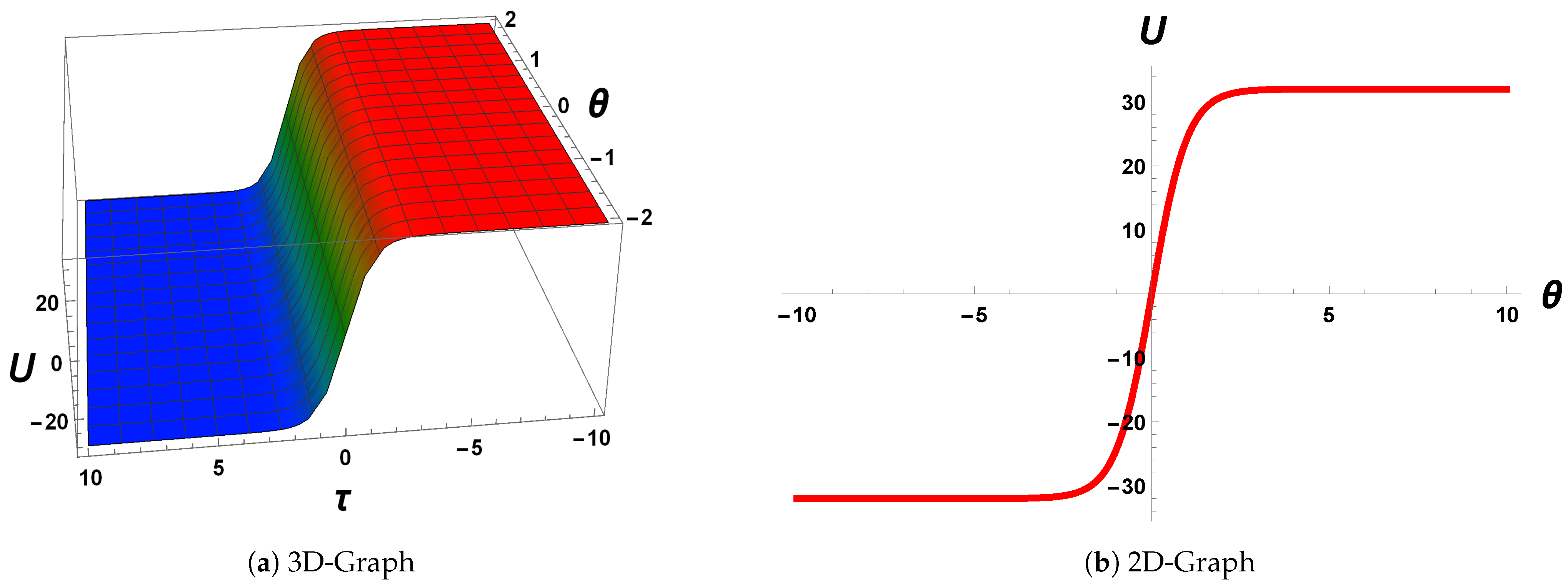
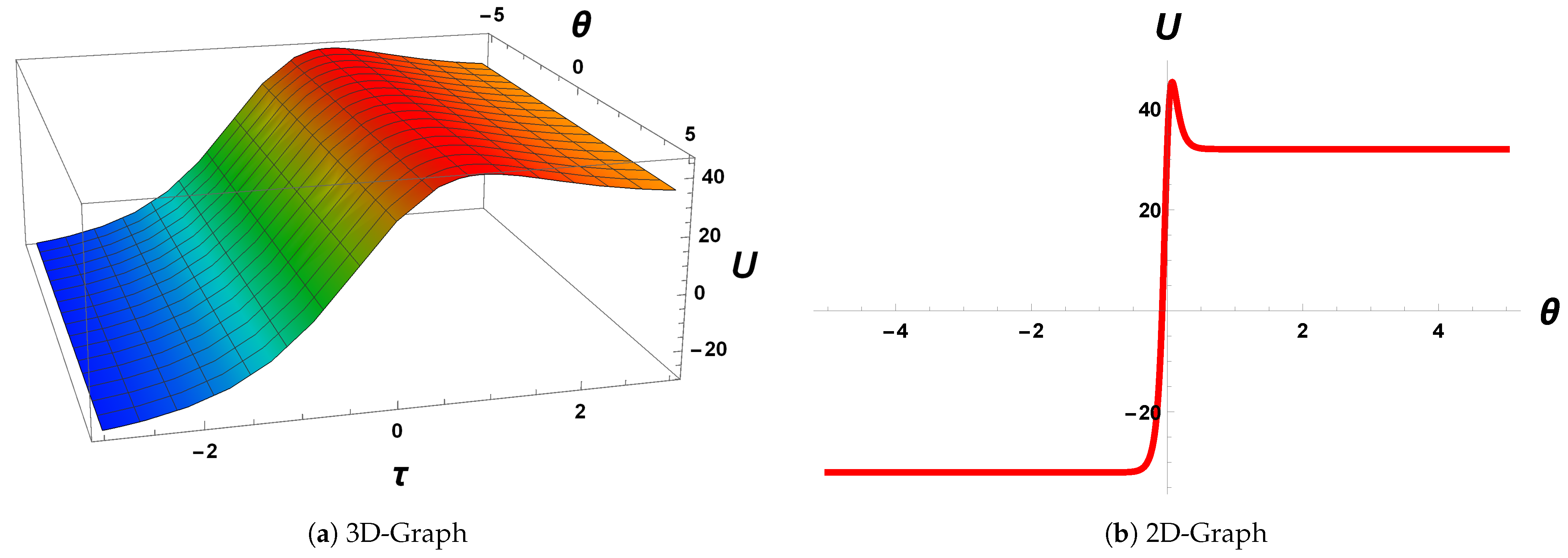
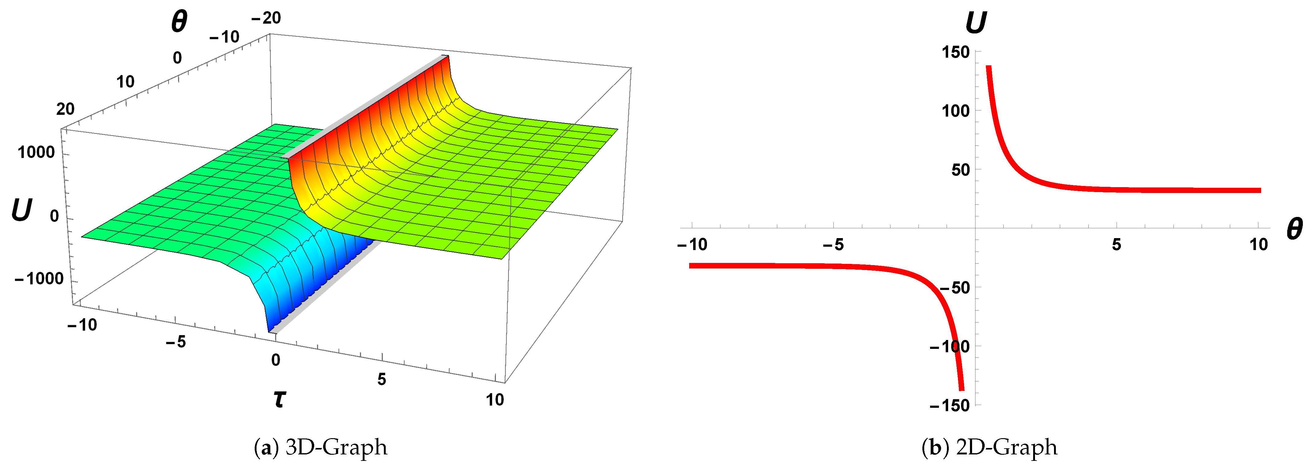
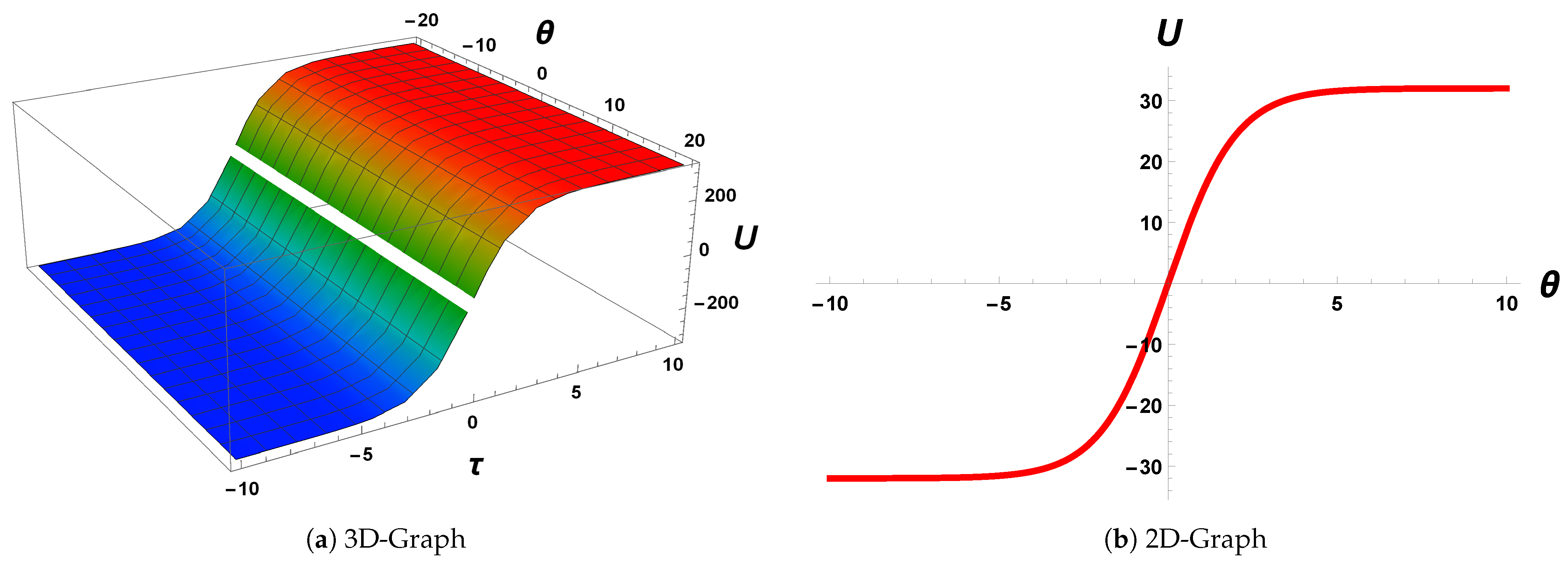
4.5. Graphical Behaviour of Wave Patterns

Here, we represent the physical importance of the considered model, some 3 D , 2 D , and density diagrams of acquired results that are plotted by using Mathematica under the suitable choice of involving parameters values. Figure 1 represent the 3 D and 2 D graph U 1 ( θ , τ ) for l 1 = 1.5 , l 2 = 0.75 , δ = 0.5 , γ 1 = 0.50 , γ 2 = 0.50 , γ 3 = 0.75 . We have shown the graphical structure of U 2 ( θ , τ ) for l 1 = 0.25 , l 2 = 0.50 , δ = 0.25 , γ 1 = 1.5 , γ 2 = 0.10 , and γ 3 = 1.5 in Figure 2.
3 D and 2 D graphical behaviour of U 4 ( θ , τ ) for l 1 = 1.5 , l 2 = 0.75 , δ = 2 , γ 1 = 2 , γ 2 = 0.5 , and γ 3 = 1.7 is shown in Figure 3 Graphical representation of U 5 ( θ , τ ) for l 1 = 1.5 , l 2 = 0.75 , δ = 0.5 , γ 1 = 0.50 , γ 2 = 0.50 , and γ 3 = 0.75 is presented in Figure 4. Furthermore, 2 D and 3 D diagrams of U 6 ( θ , τ ) for l 1 = 0.25 , l 2 = 0.50 , δ = 0.25 , γ 1 = 1.5 , γ 2 = 0.10 , and γ 3 = 1.5 are shown in Figure 5.
In Figure 6, we represent the 3 D and 2 D diagrams of U 7 ( θ , τ ) for l 1 = 1.5 , l 2 = 0.75 , δ = 2 , γ 1 = 2 , γ 2 = 0.5 , γ 3 = 1.7 . 3 D and 2 D graphical representations of U 8 ( θ , τ ) for l 1 = 0.2 , l 2 = 0.1 , δ = 1.5 , γ 1 = 0.5 , γ 2 = 0.15 , γ 3 = 1.7 are shown in Figure 7.
Figure 8 show the 3 D and 2 D diagrams of U 9 ( θ , τ ) for l 1 = 0.2 , l 2 = 0.1 , δ = 1.5 , γ 1 = 0.5 , γ 2 = 0.15 , and γ 3 = 1.7 . We represent the 3 D and 2 D diagrams of U 19 ( θ , τ ) for l 1 = 1.5 , l 2 = 0.75 , δ = 0.1 , γ 1 = 0.1 , b e t a = 0.15 , γ 3 = 1.2 in Figure 9.
Moreover, In Figure 10 and Figure 11, we have represented the 2 D comparison graphical behaviour of choosing different values of U 8 ( θ , τ ) for l 1 = 0.5 , l 1 = 1.0 , and l 1 = 1.5 and l 2 = 0.5 , l 2 = 1.0 , and l 2 = 1.5 .

5. Conservation Laws

Here the multiplier technique is used to construct the conservation laws for (1). From Equation (24), we obtain the determining equation for lambda Λ ( θ , τ , U ) :
δ δ U Λ ( θ , τ , U ) ( U τ τ l 1 ( U 2 ) τ τ + l 2 ( U 3 ) τ τ δ 2 U θ θ δ 4 12 U θ θ θ θ = 0 ) = 0 .
From Equation (21), the Euler operator is defined as
δ δ U = U D τ U τ D θ U θ + D τ 2 U τ τ + D θ 2 U θ θ + D θ D τ U τ θ + . . . ,
total derivative operator D τ and D θ can be written as with help of Equation (20):
D θ = θ + U θ U + U θ θ U θ + U τ θ U τ . . . , D τ = τ + U τ U + U τ τ U τ + U τ θ U θ . . . ,
solving Equation (42), and we obtain the eight multipliers:
Λ ( 1 ) ( θ , τ , U ) = τ , Λ ( 2 ) ( θ , τ , U ) = τ θ , Λ ( 3 ) ( θ , τ , U ) = τ sin 2 3 θ δ , Λ ( 4 ) ( θ , τ , U ) = τ cos 2 3 θ δ , Λ ( 5 ) ( θ , τ , U ) = 1 , Λ ( 6 ) ( θ , τ , U ) = θ , Λ ( 7 ) ( θ , τ , U ) = sin 2 3 θ δ , Λ ( 8 ) ( θ , τ , U ) = cos 2 3 θ δ
Equations (23) and (45) give us conservation laws. Two components, F 1 and F 2 , of the conservation laws for Equation (1).
Case 1 . Conserved vectors relating to
Λ ( 1 ) ( θ , τ , U ) = τ ,
can be written as:
F τ ( 1 ) = 3 l 2 τ U 2 U τ 2 l 1 τ U U τ l 2 U 3 + l 1 U 2 + τ U τ U , F θ ( 1 ) = τ δ 2 U θ 1 12 τ δ 4 U θ θ θ .
Case 2 . The conservation laws relating to
Λ ( 2 ) ( θ , τ , U ) = τ θ ,
can be written as:
F τ ( 2 ) = 3 l 2 τ θ U 2 U τ 2 l 1 τ θ U U τ l 2 θ U 3 + l 1 θ U 2 + τ θ U τ θ U , F θ ( 2 ) = τ δ 2 U τ θ δ 2 U θ + 1 12 τ δ 4 U θ θ 1 12 τ θ δ 4 U θ θ θ .
Case 3 . The conservation laws relating to
Λ ( 3 ) ( θ , τ , U ) = τ sin 2 3 θ δ ,
can be written as:
F τ ( 3 ) = sin 2 3 θ δ 2 l 1 τ U U τ 3 l 2 τ U 2 U τ + l 2 U 3 l 1 U 2 τ U τ + U , F θ ( 3 ) = 1 12 τ δ 3 2 3 U θ θ cos 2 3 θ δ 2 δ U θ θ θ sin 2 3 θ δ .
Case 4 . The conservation laws relating to
Λ ( 4 ) ( θ , τ , U ) = τ cos 2 3 θ δ ,
can be written as:
F τ ( 4 ) = cos 2 3 θ δ 2 l 1 τ U U τ 3 l 2 τ U 2 U τ + l 2 U 3 l 1 U 2 τ U τ + U , F θ ( 4 ) = 1 12 τ δ 3 2 3 U θ θ sin 2 3 θ δ + δ U θ θ θ cos 2 3 θ δ .
Case 5 . The conservation laws relating to
Λ ( 5 ) ( θ , τ , U ) = 1 ,
can be written as:
F τ ( 5 ) = 3 l 2 U 2 U τ 2 l 1 U U τ + U τ , F θ ( 5 ) = δ 2 U θ 1 12 δ 4 U θ θ θ .
Case 6 . The conservation laws relating to
Λ ( 6 ) ( θ , τ , U ) = θ ,
can be written as:
F τ ( 6 ) = 3 l 2 θ U 2 U τ 2 l 1 θ U U τ + θ U τ , F θ ( 6 ) = δ 2 U θ δ 2 U θ + 1 12 δ 4 U θ θ 1 12 δ 4 θ U θ θ θ .
Case 7 . The conservation laws relating to
Λ ( 7 ) ( θ , τ , U ) = sin 2 3 θ δ ,
can be written as:
F τ ( 7 ) = U τ sin 2 3 θ δ 3 l 2 U 2 + 2 l 1 U 1 , F θ ( 7 ) = 1 12 δ 3 2 3 U θ θ cos 2 3 θ δ δ U θ θ θ sin 2 3 θ δ .
Case 8 . The conservation laws relating to
Λ ( 8 ) ( θ , τ , U ) = cos 2 3 θ δ ,
can be written as:
F τ ( 8 ) = U τ cos 2 3 θ δ 3 l 2 U 2 + 2 l 1 U 1 , F θ ( 8 ) = 1 12 δ 3 δ U θ θ θ cos 2 3 θ δ + 2 3 U θ θ sin 2 3 θ δ .

6. Conclusions

In this work, we have studied the nonlinear model depicting the wave proliferation in NLETLs employing integration scheme modified Khater method. NLETLs have been discussed by the Lie analysis approach. This method is employed to analyse the NLETLs and construct the infinitesimal generators. We found the entire vector field and discuss the different solutions of the NLETLs. We can see that generated vector field forms an abelian Lie algebra. The assumed NLETLs were converted into nonlinear ODE by using an optimal system. Then, we explored the wave solutions with the help of the integration technique, namely the MKM, to solve the nonlinear partial differential depicting the wave proliferation in the NLETLs. We have used a MKM to get the new wave solutions. These results are in the form of trigonometric and hyperbolic functions. The benefits of the proposed technique are that they are simple, direct, reliable, and it addresses its wide-range appropriateness. It is hoped that our proposed technique is much better and can be used for the many types of NLPDE’s. To represent the physical importance of the considered model, some 3 D , 2 D , and density diagrams of acquired results are plotted by using Mathematica under the suitable choice of involving parameters values. We have shown some comparison graphical behaviour of the solution for taking different values of l 1 and l 2 . Further, the conservation laws of NLETLs are computed by the multiplier method.

Author Contributions

M.B.R.: Conceptualization, Investigation, Methodology, Initial writing J.A.: Data Curation, Data Anaysis, Project administration. Final checking Validation also A.J.: Software and Visualization, Supervision, Formal analysis. M.J.-U.-R.: Validation, Writing, Reviewing and Editing. All authors have read and agreed to the published version of the manuscript.

Funding

This work has been supported by the Polish National Science Centre under the grant OPUS 18 No. 2019/35/B/ST8/00980.

Institutional Review Board Statement

Not Applicable.

Informed Consent Statement

Not Applicable.

Data Availability Statement

My Manuscript has no associated data.

Acknowledgments

This work has been supported by the Polish National Science Centre under the grant OPUS 18 No. 2019/35/B/ST8/00980.

Conflicts of Interest

The authors declare that they have no known competing financial interests or personal relationships that could have appeared to influence the work reported in this paper. The Authors declares that there is no conflict of interest exists.

References

  1. Liu, J.G.; Osman, M.S.; Zhu, W.H.; Zhou, L.; Ai, G.P. Different complex wave structures described by the Hirota equation with variable coefficients in inhomogeneous optical fibers. Appl. Phys. B 2019, 125, 175. [Google Scholar] [CrossRef]
  2. Wazwaz, A.M. Partial Differential Equations and Solitary Wave’s Theory; Springer: Berlin/Heidelberg, Germany, 2009. [Google Scholar]
  3. Yang, X.J.; Tenreiro, M.J.A.; Srivastava, H.M. A new numerical technique for solving the local fractional diffusion equation: Two-dimensional extended differential transform approach. Appl. Math. Comput. 2016, 274, 143–151. [Google Scholar] [CrossRef]
  4. Abdelrahman, M.; Zahran, E.H.M.; Khater, M.M.A. The exp(-ϕ(ξ))-expansion method and its application for solving nonlinear evolution equations. Int. J. Mod. Nonlinear Theory Appl. 2015, 4, 37–47. [Google Scholar] [CrossRef] [Green Version]
  5. Akbar, M.A.; Ali, N.H.M.; Roy, R. Closed form solutions of two time fractional nonlinear wave equations. Results Phys. 2018, 9, 1031–1039. [Google Scholar] [CrossRef]
  6. Zeng, Z.; Liu, J. Solving (3 + 1)-dimensional generalized BKP equations by the improved (G/G)-expansion method. Indian J. Pure Appl. Phys. 2015, 53, 713–717. [Google Scholar]
  7. Islam, M.T.; Akbar, M.A.; Azad, A.K. Traveling wave solutions to some nonlinear fractional partial differential equations through the rational (G/G)expansion method. J. Ocean Eng. Sci. 2018, 3, 76–81. [Google Scholar] [CrossRef]
  8. Abdou, M.A.; Soliman, A.A. New exact travelling wave solutions for space-time fractional nonlinear equations describing nonlinear transmission lines. Results Phys. 2018, 9, 1497–1501. [Google Scholar] [CrossRef]
  9. Noor, N.F.M.; Haq, R.U.; Abbasb, Y.S.; Hashim, I. Heat flux performance in a porous medium embedded Maxwell fluid flow over a vertically stretched plate due to heat absorption. J. Nonlinear Sci. Appl. 2016, 9, 2986–3001. [Google Scholar] [CrossRef] [Green Version]
  10. Mohammed, M.A.; Ibrahim, A.I.N.; Siri, Z.; Noor, N.F.M. Mean Monte-Carlo finite difference method for random sampling of a nonlinear epidemic system. Sociol. Methods Res. 2016, 48, 34–61. [Google Scholar] [CrossRef]
  11. Manafian, J.; Ilhan, O.A.; Alizadeh, A. Periodic wave solutions and stability analysis for the KP-BBM equation with abundant novel interaction solutions. Phys. Scr. 2020, 95, 065203. [Google Scholar] [CrossRef]
  12. Islam, R.; Khan, K.; Akbar, M.A.; Islam, M.E.; Ahmed, M.T. Traveling wave solutions of some nonlinear evolution equations. Alex. Eng. J. 2015, 54, 263–269. [Google Scholar] [CrossRef] [Green Version]
  13. Akbar, M.A.; Ali, N.H.M. The improved F-expansion method with Riccati equation and its applications in mathematical physics. Cogent Math. 2017, 4, 1282577. [Google Scholar] [CrossRef]
  14. Zhang, S.; Li, J.; Zhang, L. A direct algorithm of exp-function method for non-linear evolution equations in fluids. Therm. Sci. 2016, 20, 881–884. [Google Scholar] [CrossRef] [Green Version]
  15. Baskonus, H.M.; Bulut, H.; Sulaiman, T.A. New complex hyperbolic structures to the Lonngren wave equation by using sine-Gordon expansion method. Appl. Math. Nonlinear Sci. 2019, 4, 129–138. [Google Scholar] [CrossRef] [Green Version]
  16. El-Sayed, M.F.; Moatimid, G.M.; Moussa, M.H.M.; El-Shiekh, R.M.; Khawlani, M.A. New exact solutions for coupled equal width wave equation and (2+1)-dimensional Nizhnik-Novikov-Veselov system using modified Kudryashov method. Int. J. Adv. Appl. Math. Mech. 2014, 2, 19–25. [Google Scholar]
  17. Mohyud-Din, S.T.; Irshad, A. Solitary wave solutions of some nonlinear PDEs arising in electronics. Opt. Quantum Electron. 2017, 49, 130. [Google Scholar] [CrossRef]
  18. Manafian, J.; Heidari, S. Periodic and singular kink solutions of the Hamiltonian amplitude equation. Adv. Math. Models Appl. 2019, 4, 134–149. [Google Scholar]
  19. Akbar, M.A.; Ali, N.H.M.; Hussain, J. Optical soliton solutions to the (2 + 1)- dimensional Chaffee-Infante equation and the dimensionless form of the Zakharov equation. Adv. Differ. Equ. 2019, 2019, 446. [Google Scholar] [CrossRef] [Green Version]
  20. Qasim, A.F.; Al-Rawi, E.S. Adomian decomposition method with modified Bernstein polynomials for solving ordinary and partial differential equations. J. Appl. Math. 2018, 2018, 1803107. [Google Scholar] [CrossRef] [Green Version]
  21. Rezazadeh, H.; Osman, M.S.; Eslami, M.; Mirzazadeh, M.; Zhou, Q.; Badri, S.A.; Korkmaz, A. Hyperbolic rational solutions to a variety of conformable fractional Boussinesqlike equations. Nonlinear Eng. 2019, 8, 224–230. [Google Scholar] [CrossRef]
  22. Ghanbari, B.; Osman, M.S.; Baleanu, D. Generalized exponential rational function method for extended Zakharov Kuznetsov equation with conformable derivative. Mod. Phys. Lett. A 2019, 34, 1950155. [Google Scholar] [CrossRef]
  23. Osman, M.S.; Rezazadeh, H.; Eslami, M. Traveling wave solutions for (3 + 1) dimensional conformable fractional Zakharov-Kuznetsov equation with power law nonlinearity. Nonlinear Eng. 2019, 8, 559–567. [Google Scholar] [CrossRef]
  24. Shahoot, A.M.; Alurrfi, K.A.E.; Hassan, I.M.; Almsri, A.M. Solitons and other exact solutions for two nonlinear PDEs in mathematical physics using the generalized projective Riccati equations method. Adv. Math. Phys. 2018, 2018, 6870310. [Google Scholar] [CrossRef]
  25. Hu, W.P.; Deng, Z.C.; Han, S.M.; Fa, W. Multi-symplectic Runge-Kutta methods for Landau Ginzburg-Higgs equation. Appl. Math. Mech. 2009, 30, 1027–1034. [Google Scholar] [CrossRef]
  26. Raslan, K.R.; Ali, K.K.; Shallal, M.A. The modified extended tanh method with the Riccati equation for solving the space-time fractional EW and MEW equations. Chaos Solitons Fractals 2017, 103, 404–409. [Google Scholar] [CrossRef]
  27. Osman, M.S. One-soliton shaping and inelastic collision between double solitons in the fifth-order variable-coefficient Sawada-Kotera equation. Nonlinear Dyn. 2019, 96, 1491–1496. [Google Scholar] [CrossRef]
  28. Lu, D.; Osman, M.S.; Khater, M.M.A.; Attia, R.A.M.; Baleanu, D. Analytical and numerical simulations for the kinetics of phase separation in iron (Fe-Cr-X (X = Mo, Cu)) based on ternary alloys. Phys. A 2020, 537, 122634. [Google Scholar] [CrossRef]
  29. Khater, M.M.A.; Mohamed, M.S.; Attia, R.A.M. On semi analytical and numerical simulations for a mathematical biological model; the time-fractional nonlinear Kolmogorov-Petrovskii-Piskunov (KPP) equation. Chaos Solitons Fractals 2021, 144, 110676. [Google Scholar] [CrossRef]
  30. Chu, Y.; Khater, M.M.A.; Hamed, Y.S. Diverse novel analytical and semi-analytical wave solutions of the generalized (2 + 1)-dimensional shallow water waves model. AIP Adv. 2021, 11, 015223. [Google Scholar] [CrossRef]
  31. Khater, M.M.A.; Ahmed, A.E.; El-Shorbagy, M.A. Abundant stable computational solutions of Atangana—Baleanu fractional nonlinear HIV-1 infection of CD4+T-cells of immunodeficiency syndrome. Result Phys. 2021, 22, 103890. [Google Scholar] [CrossRef]
  32. Khater, M.M.A.; Ahmed, A.E.; Alfalqi, S.H.; Alzaidi, J.F.; Elbendary, J.; Alabdali, A.M. Computational and approximate solutions of complex nonlinearFokas-Lenells equation arising in optical fiber. Result Phys. 2021, 25, 104322. [Google Scholar] [CrossRef]
  33. Khater, M.M.A.; Mousa, A.A.; El-Shorbagy, M.A.; Attia, R.A.M. Analytical and semi-analytical solutions for Phi-four equation through three recent schemes. Result Phys. 2021, 22, 103954. [Google Scholar] [CrossRef]
  34. Khater, M.M.A.; Nisar, K.S.; Mohamed, M.S. Numerical investigation for the fractional nonlinearspace-time telegraph equation via the trigonometricQuintic B-spline scheme. Math. Meth. Appl. Sci. 2021, 44, 4598–4606. [Google Scholar] [CrossRef]
  35. Tashlykov, O.L.; Vlasova, S.G.; Kovyazina, I.S.; Mahmoud, K.A. Repercussions of yttrium oxides on radiation shielding capacity of sodium-silicate glass system: Experimental and Monte Carlo simulation study. Eur. Phys. J. Plus. 2021, 136, 428. [Google Scholar] [CrossRef]
  36. Khater, M.M.A.; Nofal, T.A.; Abu-Zinadah, H.; Lotayif, M.S.M.; Lu, D. Novel computational and accurate numericalsolutions of the modified Benjamin-Bona-Mahony(BBM) equation arising in the optical illusions field. Alex. Eng. J. 2021, 1, 1797–1806. [Google Scholar] [CrossRef]
  37. Khater, M.M.A.; Mohamed, M.S.; Elagan, S.K. Diverse accurate computational solutions of the nonlinear Klein-Fock-Gordon equation. Result Phys. 2021, 23, 104003. [Google Scholar] [CrossRef]
  38. Khater, M.M.A.; Anwar, S.; Tariq, K.U.; Mohamed, M.S. Some optical soliton solutions to the perturbed nonlinear Schrödinger equation by modified Khater method. AIP Adv. 2021, 11, 025130. [Google Scholar] [CrossRef]
  39. Khater, M.M.A.; Bekir, A.; Lu, D.; Attia, R.A.M. Analytical and semi-analytical solutions for time-fractional Cahn-Allen equation. Math. Meth. Appl. Sci. 2021, 44, 2682–2691. [Google Scholar] [CrossRef]
  40. Wei, S.W.; Liu, Y.X. Testing the nature of Gauss–Bonnet gravity by four-dimensional rotating black hole shadow. Eur. Phys. J. Plus. 2021, 136, 436. [Google Scholar] [CrossRef]
  41. Khater, M.M.A.; Elagan, S.K.; Mousa, A.A.; El-Shorbagy, M.A.; Alfalqi, S.H.; Alzaidi, J.F.; Lu, D. Sub-10-fs-pulse propagation between analytical and numerical investigation. Result Phys. 2021, 25, 104133. [Google Scholar] [CrossRef]
  42. Zhang, X.; Shao, J.; Yan, C.; Qin, R.; Lu, Z.; Geng, H.; Xu, T.; Ju, L. A review on optoelectronic device applications of 2D transition metalcarbides and nitrides. AIP Adv. 2021, 11, 055105. [Google Scholar]
  43. Khater, M.M.A. Abundant breather and semi-analytical investigation: On high-frequency waves’ dynamics in the relaxation medium. Mod. Phys. Lett. B 2021, 35, 2150372. [Google Scholar] [CrossRef]
  44. Khater, M.M.A.; Lu, D. Analytical versus numerical solutions of the nonlinear fractional time–space telegraph equation. Mod. Phys. Lett. B 2021, 35, 2150324. [Google Scholar] [CrossRef]
  45. Khater, M.M.A.; Ahmed, A.E. Strong Langmuir turbulence dynamics through the trigonometric quintic and exponential B-spline schemes. AIMS Math. 2021, 6, 5896–5908. [Google Scholar] [CrossRef]
  46. Wang, P.; Zhang, M. Passive synchronization in optomechanical resonators coupled through an optical field. Chaos Solitons Fractals 2021, 144, 110717. [Google Scholar] [CrossRef]
  47. Abdoulkary, S.; Beda, T.; Dafounamssou, O.; Tafo, E.W.; Mohamadou, A. Dynamics of solitary pulses in the nonlinear low-pass electrical transmission lines through the auxiliary equation method. J. Mod. Phys. Appl. 2013, 2, 69–87. [Google Scholar]
  48. Malwe, B.H.; Betchewe, G.; Doka, S.Y.; Kofane, T.C. Travelling wave solutions and soliton solutions for the nonlinear transmission line using the generalized Ric- cati equation mapping method. Nonlinear Dyn. 2016, 84, 171–177. [Google Scholar] [CrossRef]
  49. Kae, A.; Mom, E.; Almsiri, A.M.; Amh, A. The expansion method for describing the nonlinear low-pass electrical lines. J Taibah Uni Sci 2019, 13, 63–70. [Google Scholar]
  50. Eme, Z.; Kae, A. The generalized projective Riccati equations method and its applications to nonlinear PDEs describing nonlinear transmission lines. Commun. Appl. Electron 2015, 3, 2394–4714. [Google Scholar]
  51. Lie, S. Theories der Tranformationgruppen, Dritter and Letzter Abschnitt; Teubner: Leipzig, Germany; Berlin, Germany, 1888. [Google Scholar]
  52. Li, C.; Zhang, J. Lie symmetry analysis and exact solutions of generalized fractional Zakharov-Kuznetsov equations. Symmetry 2019, 11, 601. [Google Scholar] [CrossRef] [Green Version]
  53. Jhangeer, A.; Hussain, A.; Junaid-U-Rehman, M.; Baleanu, D.; Riaz, M.B. Quasi-periodic, chaotic and travelling wave structures of modified Gardner equation. Chaos Solitons Fractals 2021, 143, 110578. [Google Scholar] [CrossRef]
  54. Liu, H.; Bai, C.-L.; Xin, X.; Zhang, L. A novel Lie group classification method for generalized cylindrical KdV type of equation: Exact solutions and conservation laws. J. Math. Fluid Mech. 2019, 21, 21–55. [Google Scholar] [CrossRef]
  55. Hussain, A.; Jhangeer, A.; Abbas, N. Symmetries, conservation laws and dust acoustic solitons of two-temperature ion in inhomogeneous plasma. Int. J. Geom. Methods Mod. Phys. 2021, 18, 2150071. [Google Scholar] [CrossRef]
  56. Hussain, A.; Jhangeer, A.; Abbas, N.; Khan, I.; Nisar, K.S. Solitary wave patterns and conservation laws of fourth-order nonlinear symmetric regularized long-wave equation arising in plasma. Ain Shams Eng. J. 2021. [Google Scholar] [CrossRef]
  57. Riaz, M.B.; Baleanu, D.; Jhangeer, A.; Abbas, N. Nonlinear self-adjointness, conserved vectors, and traveling wave structures for the kinetics of phase separation dependent on ternary alloys in iron (Fe-Cr-Y (Y = Mo, Cu)). Results Phys. 2021, 25, 104151. [Google Scholar] [CrossRef]
  58. Jhangeer, A.; Hussain, A.; Junaid-U-Rehman, M.; Khan, I.; Baleanu, D.; Nisar, K.S. Lie analysis, conservation laws and travelling wave structures of nonlinear Bogoyavlenskii–Kadomtsev–Petviashvili equation. Results Phys. 2020, 19, 103492. [Google Scholar] [CrossRef]
  59. Jhangeer, A.; Seadawy, A.R.; Ali, F.; Ahmed, A. New complex waves of perturbed Shrödinger equation with Kerr law nonlinearity and Kundu-Mukherjee-Naskar equation. Results Phys. 2020, 16, 102816. [Google Scholar] [CrossRef]
  60. Ibragimov, N.H. A new conservation theorem. J. Math. Anal. Appl. 2007, 333, 311–328. [Google Scholar] [CrossRef] [Green Version]
  61. Olver, P.J. Application of Lie Groups to Differential Equations; Springer: New York, NY, USA, 1993. [Google Scholar]
  62. Bluman, G.W.; Cheviakov, A.F.; Anco, S.C. Applications of Symmetry Methods to Partial Differential Equations; Springer: Berlin/Heidelberg, Germany, 2000. [Google Scholar]
  63. Ovsiannikov, L.V. Group Analysis of Differential Equations; Academic: New York, NY, USA, 1982. [Google Scholar]
  64. El-Ganaini, S.; Kumar, H. A variety of new traveling and localized solitary wave solutions of a nonlinear model describing the nonlinear low- pass electrical transmission lines. Chaos Solitons Fractals 2020, 140, 110218. [Google Scholar] [CrossRef]
  65. Eme, Z.; Kae, A. A new Jacobi elliptic function expansion method for solving a nonlinear PDE describing the nonlinear low-pass electrical lines. Chaos Solitons Fractals 2015, 78, 148–155. [Google Scholar]
  66. Jhangeer, A.; Rezazadeh, H.; Abazari, R.; Yildirim, K.; Sharif, S.; Ibraheem, F. Lie analysis, conserved quantities and solitonic structures of Calogero-Degasperis-Fokas equation. Alex. Eng. J. 2021, 60, 2513–2523. [Google Scholar] [CrossRef]
  67. Naz, R.; Mahomed, F.M.; Mason, D.P. Comparison of different approaches to conservation laws for some partial differential equations in fluid mechanics. Appl. Math. Comp. 2008, 205, 212–230. [Google Scholar] [CrossRef]
  68. Hereman, W. Symbolic computation of conservation laws of nonlinear partial differential equations in multi-dimensions. Int. J. Quantum Chem. 2006, 106, 278–299. [Google Scholar] [CrossRef] [Green Version]
  69. Cheviakov, A.F. GeM software package for computation of symmetries and conservation laws of differential equations. Comput. Phys. Comm. 2007, 176, 48–61. [Google Scholar] [CrossRef]
  70. Cheviakov, A.F. Computation of fluxes of conservation laws. J. Eng. Math. 2010, 66, 153–173. [Google Scholar] [CrossRef] [Green Version]
  71. Hussain, A.; Jhangeer, A.; Abbas, N.; Khan, I.; Sherif, E.S.M. Optical solitons of fractional complex Ginzburg-Landau equation with conformable, beta, and M-truncated derivatives: A comparative study. Adv. Differ. Equ. 2020, 2020, 1–19. [Google Scholar] [CrossRef]
  72. Anco, S.C.; Bluman, G. Direct construction method for conservation laws of partial differential equations Part II: General treatment. Eur. J. Appl. Math. 2002, 41, 567–585. [Google Scholar] [CrossRef] [Green Version]
Figure 1. Diagrams a—3D and b—2D representation of U1(θ, τ) for l1 = 1.5, l2 = 0.75, δ = 0.50, γ1 = 0.5, γ2 = 0.50, and γ3 = 0.75.
Fractalfract 05 00170 g001
Figure 2. Diagrams a—3D and b—2D representation of U2(θ, τ) for l1 = 0.25, l2 = 0.50, δ = 0.25, γ1 = 1.5, γ2 = 0.10, and γ3 = 1.5.
Fractalfract 05 00170 g002
Figure 3. Diagrams a—3D and b—2D representation of U4(θ, τ) for l1 = 1.5, l2 = 0.75, δ = 2, γ1 = 2, γ2 = 0.50, and γ3 = 1.7.
Fractalfract 05 00170 g003
Figure 4. Diagrams a—3D and b—2D representation of U5(θ, τ) for l1 = 1.5, l2 = 0.75, δ = 0.50, γ1 = 0.50, γ2 = 0.50, and γ3 = 0.75.
Fractalfract 05 00170 g004
Figure 5. Diagrams a—3D and b—2D representation of U6(θ, τ) for l1 = 0.25, l2 = 0.50, δ = 0.25, γ1 = 1.5, γ2 = 0.10, and γ3 = 1.5.
Fractalfract 05 00170 g005
Figure 6. Diagrams a—3D and b—2D representation of U7(θ, τ) for l1 = 1.5, l2 = 0.75, δ = 2, γ1 = 2, γ2 = 0.5, and γ3 = 1.7.
Fractalfract 05 00170 g006
Figure 7. Diagrams a—3D and b—2D representation of U8(θ, τ) for l1 = 0.2, l2 = 0.1, δ = 1.5, γ1 = 0.5, γ2 = 0.15, and γ3 = 1.7.
Fractalfract 05 00170 g007
Figure 8. Diagrams a—3D and b—2D representation of U9(θ, τ) for l1 = 0.2, l2 = 0.1, δ = 1.5, γ1 = 0.5, γ2 = 0.15, and γ3 = 1.7.
Fractalfract 05 00170 g008
Figure 9. Diagrams a—3D and b—2D representation of U19(θ, τ) for l1 = 1, l1 = 1.5, l2 = 0.75, δ = 0.1, γ1 = 0.1, γ2 = 0.15, and γ3 = 1.2.
Fractalfract 05 00170 g009
Figure 10. Comparison of different values if l 1 .
Fractalfract 05 00170 g010
Figure 11. Comparison of different values if l 2 .
Fractalfract 05 00170 g011
Publisher’s Note: MDPI stays neutral with regard to jurisdictional claims in published maps and institutional affiliations.

