Article

Quarter-Sweep Preconditioned Relaxation Method, Algorithm and Efficiency Analysis for Fractional Mathematical Equation

1
Tadris Matematika, IAIN Bengkulu, Bengkulu 38211, Indonesia
2
Department of Mathematics, Anand International College of Engineering, Jaipur 303012, India
3
Nonlinear Dynamics Research Center (NDRC), Ajman University, Ajman 346, United Arab Emirates
4
International Center for Basic and Applied Sciences, Jaipur 302029, India
5
Faculty of Science and Natural Resources, Universiti Malaysia Sabah, Kota Kinabalu 88400, Malaysia
6
Faculty of Computing and Informatics, Universiti Malaysia Sabah Labuan International Campus, Labuan 87000, Malaysia
7
Department of Mathematics, Faculty of Science, University of Jordan, Amman 11942, Jordan
*
Authors to whom correspondence should be addressed.
Fractal Fract. 2021, 5(3), 98; https://doi.org/10.3390/fractalfract5030098
Submission received: 23 June 2021 / Revised: 5 August 2021 / Accepted: 10 August 2021 / Published: 14 August 2021

Abstract

:
Research into the recent developments for solving fractional mathematical equations requires accurate and efficient numerical methods. Although many numerical methods based on Caputo’s fractional derivative have been proposed to solve fractional mathematical equations, the efficiency of obtaining solutions using these methods when dealing with a large matrix requires further study. The matrix size influences the accuracy of the solution. Therefore, this paper proposes a quarter-sweep finite difference scheme with a preconditioned relaxation-based approximation to efficiently solve a large matrix, which is based on the establishment of a linear system for a fractional mathematical equation. The paper presents the formulation of the quarter-sweep finite difference scheme that is used to approximate the selected fractional mathematical equation. Then, the derivation of a preconditioned relaxation method based on a quarter-sweep scheme is discussed. The design of a C++ algorithm of the proposed quarter-sweep preconditioned relaxation method is shown and, finally, efficiency analysis comparing the proposed method with several tested methods is presented. The contributions of this paper are the presentation of a new preconditioned matrix to restructure the developed linear system, and the derivation of an efficient preconditioned relaxation iterative method for solving a fractional mathematical equation. By simulating the solutions of time-fractional diffusion problems with the proposed numerical method, the study found that computing solutions using the quarter-sweep preconditioned relaxation method is more efficient than using the tested methods. The proposed numerical method is able to solve the selected problems with fewer iterations and a faster execution time than the tested existing methods. The efficiency of the methods was evaluated using different matrix sizes. Thus, the combination of a quarter-sweep finite difference method, Caputo’s time-fractional derivative, and the preconditioned successive over-relaxation method showed good potential for solving different types of fractional mathematical equations, and provides a future direction for this field of research.

1. Introduction

Research into the recent developments for solving fractional mathematical equations requires accurate and efficient numerical methods. The accuracy and efficiency of the numerical method used to solve a fractional mathematical equation determine the precision when interpreting the behaviours of physical phenomena. Accurate and efficient methods enable researchers to explore and solve a greater number of complex fractional mathematical models. Many numerical methods based on Caputo’s fractional derivative have been proposed to approximate the solution of the modelled fractional mathematical equations. For instance, ref. [1] proposed two numerical methods, the non-standard finite difference method and the generalized Euler method, for solving a mathematical model of drug resistance during treatment for human immunodeficiency virus, using the Caputo approach. Subsequently, ref. [2] studied the conversion of an existing tobacco smoking model into a fractional-order Caputo model, and used the combination of the fourth-order Runge–Kutta and Adams–Bashforth–Moulton methods to solve the developed model. In another article, ref. [3] developed a time–space fractional hyperbolic bioheat transfer model for non-Fourier bioheat transfer in living biological tissues during laser irradiation using Caputo’s definition. They applied an L1 finite difference approximation to Caputo’s time-fractional derivative and a central difference approximation to Riesz’s space-fractional derivative for the solution of the model. In addition, ref. [4] investigated Caputo’s fractional Maxwell model of unsteady fluid flow and heat transfer of the natural convection of a viscoelastic non-Newtonian fluid using a finite difference method.
Of the many existing numerical methods, the finite difference method, widely known as FDM, is one of the most popular numerical methods used to solve fractional mathematical equations using the Caputo approach. From our review of several applications of FDM to solve Caputo’s time-fractional mathematical equations, ref. [5] utilized the implicit FDM to solve the time-fractional diffusion equation with a time-invariant type variable. Subsequently, ref. [6] developed a fourth-order FDM to solve a time-fractional diffusion equation after transforming the fractional mathematical equation into a Volterra integro-differential equation via a Laplace transform. In addition, ref. [7] proposed a weighted FDM to effectively solve a system of variable-order time-fractional two-dimensional Burgers’ equations. FDM can also be combined with spline approximation to solve the time-fractional stochastic advection equation [8]. These studies are examples of the numerous works published by global researchers. The abundance of related research in the literature has motivated numerous researchers to propose more accurate and efficient numerical methods for solving fractional mathematical equations.
In our view, the efficiency of numerical methods used to obtain the solution of a fractional mathematical equation when dealing with a large matrix requires further study because the accuracy of the solution is influenced by the matrix size. Therefore, this paper proposes a quarter-sweep finite difference scheme with a preconditioned relaxation-based approximation to efficiently solve a large matrix, which results from establishing a linear system for a fractional mathematical equation. The quarter-sweep finite difference scheme is suitable for solving a fractional mathematical equation because, among other reasons, the derivation of the scheme is similar to that of an implicit FDM, which makes it compatible with Caputo’s time-fractional approximation. The quarter-sweep scheme is derived by modifying an implicit FDM by skipping three grid points for two consecutive unknown grid points. The values of the unknown grid points can be computed using the iterative method until they converge. Then, the remaining grid points resulting from the skipping procedure are computed directly using the approximation function [9,10,11]. Moreover, due to the combination of iterative and direct computation, the quarter-sweep scheme has a lower computational burden compared to the implicit and high-order FDM. This paper introduces a preconditioned relaxation method to improve the convergence rate of the iterations, thereby resulting in a highly efficient numerical method. The contributions of the paper are the presentation of a new preconditioned matrix to restructure the developed linear system and the derivation of an efficient preconditioned relaxation iterative method for solving a fractional mathematical equation.
To investigate the efficacy of this new numerical method, a well-known fractional mathematical equation, namely, the fractional diffusion equation (FDE), was selected as a mathematical problem. FDE is a fractional mathematical equation that has been successfully used in the mathematical modelling of physical phenomena. Due to the limitation of the classic diffusion equation in the modelling of the anomalous diffusion process, the theory and application of fractional diffusion have evolved. Hence, FDE has been used to successfully model shipping water events [12], image denoising [13], dye-sensitized solar cells [14], diffusion of soluble substances [15], groundwater pollution [16], option pricing and risk calculation [17], and signal smoothing performance analysis [18]. A better understanding of FDE models can be achieved using an efficient numerical method called the quarter-sweep preconditioned relaxation method. It should be noted that this paper extends the works from [19] and [20], which implemented the standard implicit FDM with preconditioned relaxation and the half-sweep difference scheme with preconditioned relaxation, respectively, for solving the time FDE. The work in [19] showed the improvement in the number of iterations and execution time after implementing a preconditioned successive over-relaxation with implicit FDM using the Caputo approach to solve the time FDE. Another article [20] applied a computational complexity reduction technique called the half-sweep iteration to successfully reduce the computational cost using preconditioned successive over-relaxation, and eventually improve the efficiency of Caputo’s finite difference scheme. This paper extends these works by employing the quarter-sweep FDM to reduce the computational cost of solving the FDE using a preconditioned successive over-relaxation when dealing with a large matrix.
This paper is organized as follows: Section 2 presents Caputo’s fractional operator, one of the important definitions in the fractional derivative theory. In Section 3, an approximation to a general time FDE is formulated using Caputo’s fractional operator and the quarter-sweep numerical discretization procedure. Section 4 explains the stability of the approximation to the considered mathematical equation. Section 5 discusses the convergence of the quarter-sweep finite difference approximation in the Caputo sense. In Section 6, the concept of preconditioned successive over-relaxation (PSOR) used to formulate the quarter-sweep PSOR (QSPSOR) iterative method is discussed. Section 7 shows the implementation and application of an algorithm written in C++ programming language for the numerical experiment and simulation with QSPSOR, and provides a comparison with selected existing methods. Finally, a conclusion is given in Section 8.

2. Preliminary

Formulating a quarter-sweep approximation to a time FDE requires good knowledge of fractional calculus theory and several useful operators. In the preliminary stage of this paper, Caputo’s fractional operator is used to approximate the time-fractional derivative term. The definition of Caputo’s derivative with a fractional order is as follows:
Definition 1
([21]).Let m 1 < α < m , where m is an element of the set of natural numbers, and α is a real number, and a function f ( x ) such that D 0 α f ( x ) exists. Caputo’s fractional operator can be defined in the form of:
D 0 α f ( x ) = 0 x f ( m ) ( r ) ( x r ) α ( m 1 )   d r .
Using Definition 1, a time-fractional derivative term in a differential equation can be approximated by:
D t α z ( x , t ) = 1 Γ ( 1 α ) 0 t z ( x , τ ) t ( t τ ) α   d τ ,
where 0 < α < 1 and z ( x , t ) > 0 .
The next section discusses the formulation of a quarter-sweep finite difference approximation to the time FDE, which uses Equation (2) to approximate the time-fractional derivative.

3. Mixed Caputo Fractional Operator and Quarter-Sweep Discretization Scheme

To demonstrate the formulation of the mixed Caputo fractional operator and quarter-sweep discretization scheme, let us consider a well-known model of the time FDE, namely:
α z ( x , t ) t α = a ( x ) 2 z ( x , t ) x 2 + b ( x ) z ( x , t ) x + c ( x ) z ( x , t ) ,
where a ( x ) ,   b ( x ) , and c ( x ) are either predefined functions, constants, or mixed.
A suitable boundary condition must be imposed on Equation (3) before the solution can be derived using an FDM. In this paper, a Dirichlet-type boundary condition is used to construct a solution domain. Furthermore, the solution domain is restricted to the usual finite domain 0 x γ because the aim of this paper is to investigate of the efficacy of a new iterative method developed from the use of Equation (2) and a quarter-sweep FDM. Based on Equation (3), Caputo’s fractional approximation to the fractional order in time is illustrated as follows:
α z ( x i , t n ) t α = 1 Γ ( 1 α ) 0 t n z ( x i , τ ) t ( t n τ ) α   d τ .
Equation (4) can be derived further and simplified to:
α z ( x i , t n ) t α = 1 Γ ( 1 α ) ( 1 α ) k α j = 1 n ( Z i , j Z i , j 1 ) [ ( n ( j 1 ) ) 1 α ( n j ) 1 α ] + 1 Γ ( 1 α ) ( 1 α ) j = 1 n [ ( n ( j 1 ) ) 1 α ( n j ) 1 α ] O ( k 2 α ) .
Next, by defining:
σ α , k = 1 Γ ( 1 α ) ( 1 α ) k α ,
where k is a real number, and:
ω α , j = j 1 α ( j 1 ) 1 α ,
a discrete approximation to the fractional order in time becomes:
α z ( x i , t n ) t α = σ α , k j = 0 n ω α , j ( Z i , n ( j 1 ) Z i , n j ) + 1 Γ ( 1 α ) ( 1 α ) n 1 α O ( k 2 α ) ,
and, finally:
α z ( x i , t n ) t α = σ α , k j = 0 n ω α , j ( Z i , n ( j 1 ) Z i , n j ) + O ( k ) .
To discretize the right-hand side part of Equation (3) using a quarter-sweep implicit scheme of FDM, let the solution domain of the problem be partitioned uniformly. Let some integers M > 0 and N > 0 denote the grid sizes in space and time, respectively. Similar to the standard finite difference framework, we use h = γ / M and k = T / N , respectively. Then, a uniform mesh of the solution can be formed using the distributed points in the space [ 0 ,   γ ] as x i = i h , i = 1 , 2 , , M 1 , and the distributed points in the time [ 0 ,   T ] are labelled t n = n k , n = 1 , 2 , , N . All of the unknown values of the solution function z ( x i , t n ) located at these grid points are represented by Z i , n .
Using Equation (9), in combination with a quarter-sweep implicit scheme, the quarter-sweep Caputo fractional approximation of Equation (3) to the point centered at z ( x i , t n ) = z ( i h , n k ) can be formulated and written as:
σ α , k j = 0 n   ω α , j ( Z i , n ( j 1 ) Z i , n j ) + O ( k ) = a i 16 h 2 ( Z i 4 , n 2 Z i , n + Z i + 4 , n ) + b i 8 h ( Z i + 4 , n Z i 4 , n ) + c i Z i , n + O ( h 2 ) ,
where i = 4 , 6 , m 4 .
The approximation structure presented in Equation (10) is similar to a standard implicit approximation equation, with the exception that the distance between any two points is quadrupled. Equation (10) is also consistent with the first-order accuracy in time and second-order accuracy in space. When Equation (10) is written in a particular form, for instance, at time level n 2 , one can obtain:
σ α , k j = 2 n   ω α , j ( Z i , n ( j 1 ) Z i , n j ) = a i Z i 4 , n + b i Z i , n + c i Z i + 4 , n ,
where:
a i = a i 16 h 2 b i 8 h ,   b i = c i a i 8 h 2 ,   c i = a i 16 h 2 + b i 8 h .
Moreover, for n = 1 , one can obtain:
F i , 1 = a i Z i 4 , 1 + b i Z i , 1 c i Z i + 4 , 1 ,
where:
b i = σ α , k b i , F i , 1 = σ α , k Z i , 0 .
Furthermore, using Equation (14), a corresponding linear system can be constructed properly in the form of a matrix as:
A Z ˜ = F ˜ ,
where:
A = [ b 4 c 4 a 8 b 8 c 8 a 12 b 12   c 12 a M 8 b M 8 a M 4 c M 8 b M 4 ] ,
Z ˜ = [ Z 4 , 1 ,   Z 8 , 1 ,   Z 12 , 1 , , Z M 8 , 1 , Z M 4 , 1 ] T ,
and:
F ˜ = [ F 4 , 1 + a 4 F 0 , 1 ,   F 8 , 1 ,   F 12 , 1 , , F M 8 , 1 , F M 4 , 1 + c M 4 F M , 1 ] T .

4. Stability of Caputo’s Fractional Approximation with a Quarter-Sweep Scheme

This section discusses the stability analysis of the quarter-sweep Caputo fractional approximation to the time FDE as shown in Equation (3). In this paper, two common stability verification approaches are applied: Von Neumann’s method and the Lax equivalence theorem. The developed theorem for the stability of the quarter-sweep Caputo fractional approximation is presented below.
Theorem 1.
The quarter-sweep implicit approximation with Caputo’s fractional operator for 0 < α < 1 , on the finite space 0 x 1 and all t > 0 , is unconditionally stable.
Proof of Theorem 1.
Suppose that a solution function of Equation (3) has the form:
Z i , n = ξ n e I ( λ i h ) ,
where I = 1 and λ is a real number. Using Equation (19), the quarter-sweep Caputo fractional approximation shown by Equation (11) can be rewritten as:
σ α , k j = 2 n ω α , j ( ξ n ( j 1 ) e I ( λ i h ) ξ n j e I ( λ i h ) ) = a i ξ n e I ( λ ( i 4 ) h ) + b i ξ n e I ( λ i h ) + c i ξ n e I ( λ ( i + 4 ) h ) .
Equation (20) can be transformed into:
σ α , k ξ n 1 e I ( λ i h ) + σ α , k j = 2 n   ω α , j ( ξ n ( j 1 ) e I ( λ i h ) ξ n j e I ( λ i h ) ) = a i ξ n e I ( λ ( i 4 ) h ) + ( b i σ α , k ) ξ n e I ( λ i h ) + c i ξ n e I ( λ ( i + 4 ) h ) .
By simplifying and rearranging the distinct terms in Equation (21), one can obtain:
σ α , k ξ n 1 + σ α , k j = 2 n ω α , j ( ξ n ( j 1 ) ξ n j ) = ξ n ( ( ( a i + c i ) cos 4 λ h ) + ( b i σ α , k ) ) ,
which can be reduced to:
ξ n = ξ n 1 + j = 2 n   ω α , j ( ξ n j ξ n ( j 1 ) ) ( 1 ( a i + c i ) cos 4 λ h + b i σ α , k ) .
From Equation (23), for all values of j ,   n ,   ω , α ,   λ , h , σ , and k , it follows that:
ξ 1 ξ 0 ,
and when n = 2 , we have:
ξ 2 ξ 1 + ω α , 2 ( ξ 0 ξ 1 ) ,
which can generally be stated as:
ξ n ξ n 1 + j = 2 n   ω α , j ( ξ n j ξ n ( j 1 ) ) , n 2 .
Since:
ξ n ξ n 1 + j = 2 n ω α , j ( ξ n j ξ n ( j 1 ) ) ξ n j ,
the inequalities in Equations (24)–(26) imply:
ξ n ξ n 1 ξ n 2 ξ 1 ξ 0 .
Thus, the stability of the quarter-sweep scheme via Caputo’s time-fractional operator is established as:
ξ n = | Z i , n | ξ 0 = | Z i , 0 | .
 □

5. Convergence of Caputo’s Fractional Approximation with a Quarter-Sweep Scheme

This section discusses the convergence analysis of the quarter-sweep Caputo fractional approximation to the time FDE in Equation (3). To begin the analysis, we define e i , n = z ( x i , t n ) Z i , n , i = 1 , 2 , , M 1 , n = 1 , 2 , , N , where z i , n and Z i , n are the exact and approximate solutions, respectively. Substitution of e i , n into Equations (11) and (13) gives:
σ α , k j = 2 n   ω α , j ( e i , n ( j 1 ) e i , n j ) = a i e i 4 , n + b i e i , n + c i e i + 4 , n + R i , n , n 2 ,
where:
R i , n = σ α , k j = 2 n   ω α , j ( z ( x i , t n ( j 1 ) ) z ( x i , t n j ) ) a i z ( x i 4 , t n ) b i z ( x i , t n ) c i z ( x i + 4 , t n ) ,
and:
σ α , k e i , 0 = a i e i 4 , 1 + ( σ α , k b i ) e i , 1 c i e i + 4 , 1 + R i , 1 .
Then, we have:
α z ( x i , t n ) t α + C 1 k = σ α , k j = 0 n ω α , j ( z ( x i , t n ( j 1 ) ) z ( x i , t n j ) ) ,
and the quarter-sweep first and second-order central difference operators as follows:
2 z ( x i , t n ) x 2 + C 2 h 2 = z ( x i 4 , t n ) 2 z ( x i , t n ) + z ( x i + 4 , t n ) 16 h 2 ,
and:
z ( x i , t n ) x + C 3 h = z ( x i 4 , t n ) z ( x i + 4 , t n ) 8 h .
Hence:
R i , n = 1 σ α , k [ α z ( x i , t n ) t α a ( x ) 2 z ( x i , t n ) x 2 b ( x ) z ( x i , t n ) x c ( x ) z ( x i , t n ) ] + C 1 k 1 + α + k α ( C 2 h 2 + C 3 h ) ,
and also:
| R i , n | C ( k 1 + α + k α ( h 2 + h ) ) , i = 1 , 2 , M 1 , n = 1 , 2 , , N ,
where C is an arbitrary constant.
Because k n N is finite, we obtain the following theorem.
Theorem 2.
Let Z i , n be the approximation of the exact value z ( x i , t n ) , computed by the quarter-sweep implicit approximation with Caputo’s fractional operator. Then, there is a positive constant C such that:
| z ( x i , t n ) Z i , n | C ( k + h 2 ) , i = 1 , 2 , M 1 , n = 1 , 2 , , N .

6. Concept and Formulation of Quarter-Sweep Preconditioned Relaxation Method

The presented PSOR iterative method is a continuation of the derivation of the quarter-sweep finite difference approximation via Caputo’s fractional derivative. The formulation of the PSOR method begins with the linear system, as shown by Equation (15). The coefficient matrix considered in Equation (15) has a large scale and is sparse. Thus, the proposed PSOR iterative method solves Equation (15) using the following matrix restructure. Firstly, a preconditioned linear system can be defined as:
A Z ˜ = F ˜ ,
where the new matrices A = P A P T ,   F ˜ = P F ˜ , and Z ˜ = P T ψ . The preconditioned matrix labelled P that is used in this paper is given by:
P = I + S ,
where:
S = [ 0 r 1 0 0 0 0 0 0 r 2 0 0 0 0 0 0 r 3 0 0 0 0 0 0 0 0 0 0 r m 1 0 0 0 0 0 0 ] .
Secondly, let us consider that the new coefficient matrix A in Equation (39) can be defined as the summation of the matrix components of:
A = D i L o V a ,
where D i , L o , and V a are diagonal, lower triangular, and upper triangular matrices, respectively. By combining Equations (39) and (42), the resultant QSPSOR iteration method can be derived as:
ψ ( η + 1 ) = ( D i ω L o ) 1 ( ( 1 ω ) D i + ω V a ) ψ ( η ) + ( D i ω L o ) 1 F ˜ ,
where ψ ( η + 1 ) represents an unknown vector at the ( η + 1 ) th iteration. The algorithm of the QSPSOR method used to compute the solution of the time FDE is described in the following Table 1.

7. Implementation and Application of C++ for Numerical Experiment

In this work, the C++ programming language was applied to implement the designed QSPSOR computational algorithm. C++ is a high-level programming language used in the field of numerical analysis. The C++ language also facilitates low-level coding because it is an extension of the medium-level programming language, C. Because C++ has all of the features and advantages of C, C++ enables the manipulation of low-level memory and the development of numerical iterative formulas to solve mathematical problems. In this work, the C++ simulation code was written to prioritize performance, speed, efficiency, and flexibility of use. Hence, implementing the quarter-sweep approximation based on Caputo’s fractional operator via the QSPSOR C++ code can yield important data, such as the number of iterations, execution time, and absolute errors.
For the numerical experiment, two problems of the time-fractional diffusion equation were selected to test the performance of the QSPSOR. For the efficiency comparison and analysis, two existing methods from our previous work were used, abbreviated as FSPSOR [19] and HSPSOR [20]. To compare the performance of these methods, three criteria were considered, namely, η —representing the number of iterations, s e c . —representing the execution time of the C++ simulation code, and ε ^ —representing the magnitude of the absolute error. The three criteria for comparison and efficiency analysis were observed and taken based on three different values of fractional order, namely, α = 0.25 , α = 0.50 , and α = 0.75 . Moreover, the simulation considered five different grid points, M = 128 ,   256 ,   512 ,   1024 , and 2048 . The problems are considered below.
Example 1
([22]).Let the time-fractional initial boundary value problem be:
α z ( x , t ) t α = 2 z ( x , t ) x 2 , 0 < α 1 , 0 x γ , t > 0 ,
where the boundary conditions are stated in fractional terms:
z ( 0 , t ) = 2 k t α Γ ( α + 1 ) , z ( γ , t ) = γ 2 + 2 k t α Γ ( α + 1 ) ,
and the initial condition is:
z ( x , 0 ) = x 2 .
The analytical solution of Equation (44) is given by:
z ( x , t ) = x 2 + 2 k t α Γ ( α + 1 ) .
Example 2
([22]).Let the next time-fractional initial boundary value problem be given as:
α z ( x , t ) t α = 1 2 x 2 2 z ( x , t ) x 2 , 0 < α 1 , 0 x γ , t > 0 ,
where the boundary conditions are given in fractional terms:
z ( 0 , t ) = 0 , z ( 1 , t ) = e t ,
and the initial condition is given by:
z ( x , 0 ) = x 2 .
The exact solution of Equation (38) is:
z ( x , t ) = x 2 e t .
The collected numerical results of the implementation of FSPSOR, HSPSOR, and QSPSOR to solve Examples 1 and 2 are recorded in Table 2 and Table 3, respectively. Based on Table 2 and Table 3, it can be observed that the QSPSOR method requires fewer iterations to obtain satisfactorily accurate approximate solutions of Examples 1 and 2. This significant improvement in the number of iterations results in a shorter execution time, which indicates QSPSOR can more efficiently solve Examples 1 and 2 than the two tested methods. The accuracy of the solution obtained by the QSPSOR method is comparable and almost equivalent to those of the FSPSOR and HSPSOR methods. A comparison of the different fractional orders of the selected examples shows that the accuracy of the solutions of the three numerical methods, which are based on the implicit finite difference scheme and Caputo’s time-fractional approximation, is greatest at α = 0.50 , followed by α = 0.75 and α = 0.25 . Although the QSPSOR method can solve the selected problems efficiently, the magnitude of the absolute errors of the solutions is slightly bigger than those of the FSPSOR and HSPSOR methods. Thus, the use of the quarter-sweep scheme as the complexity reduction approach for solving time-fractional behavior is a disadvantage due to the less effective direct computation of the remaining points. Future work will further investigate the appropriate treatment to reduce the absolute errors of the quarter-sweep difference scheme in the Caputo sense.
In addition, Figure 1, Figure 2, Figure 3 and Figure 4 show the performance graphs of the number of iterations and the execution time of the three methods. These graphs provide illustrations of the differences in terms of the efficiency of the combination of Caputo’s time-fractional approximation and preconditioned iterations via three different schemes: the standard implicit, half-sweep, and quarter-sweep. The percentage improvement in terms of the number of iterations for the proposed QSPSOR method, at α = 0.25 , indicated that the number of iterations declined significantly, by 74.64% and 53.18%, compared to the FSPSOR and HSPSOR methods, respectively. Similarly, for execution time, the QSPSOR method was significantly faster, by 90.71% and 76.18%, than the FSPSOR and HSPSOR methods, respectively. At α = 0.50 , the number of iterations needed by QSPSOR was 82.26% and 59.95% less than that required by the FSPSOR and HSPSOR methods, respectively. As a result, the C++ program execution time was 81.83% and 59.35% faster than that of the FSPSOR and HSPSOR methods, respectively. Finally, for the fractional-order α = 0.75 , QSPSOR required 86.67% and 66.69% fewer iterations than the FSPSOR and HSPSOR methods, respectively, and the C++ program execution was 79.62% and 62.49% quicker than that of the FSPSOR and HSPSOR methods, respectively.

8. Conclusions

This paper discusses and presents the numerical solution of a fractional mathematical equation, namely, the time FDE, using a quarter-sweep mixed Caputo time-fractional approximation, and a C++ program to implement the QSPSOR iterative method. A preconditioned matrix was successfully implemented to modify the matrix structure to improve the convergence rate, and the QSPSOR method was formulated to efficiently solve the matrix. A numerical experiment using two alternative methods, namely FSPSOR and HSPSOR, showed the superiority of the proposed QSPSOR method in terms of the efficiency of solving two time-fractional initial boundary value problems of the diffusion equation. The findings of this paper can be highlighted as follows:
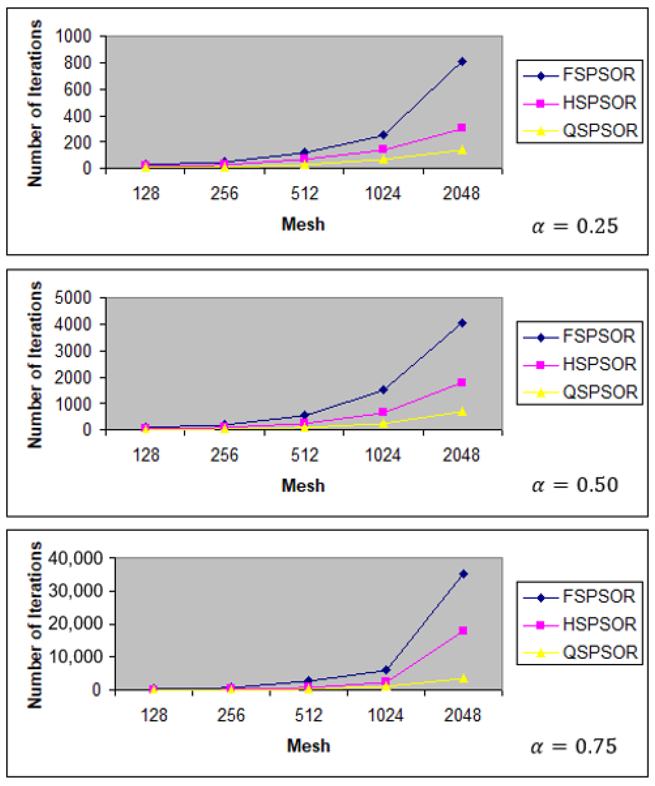
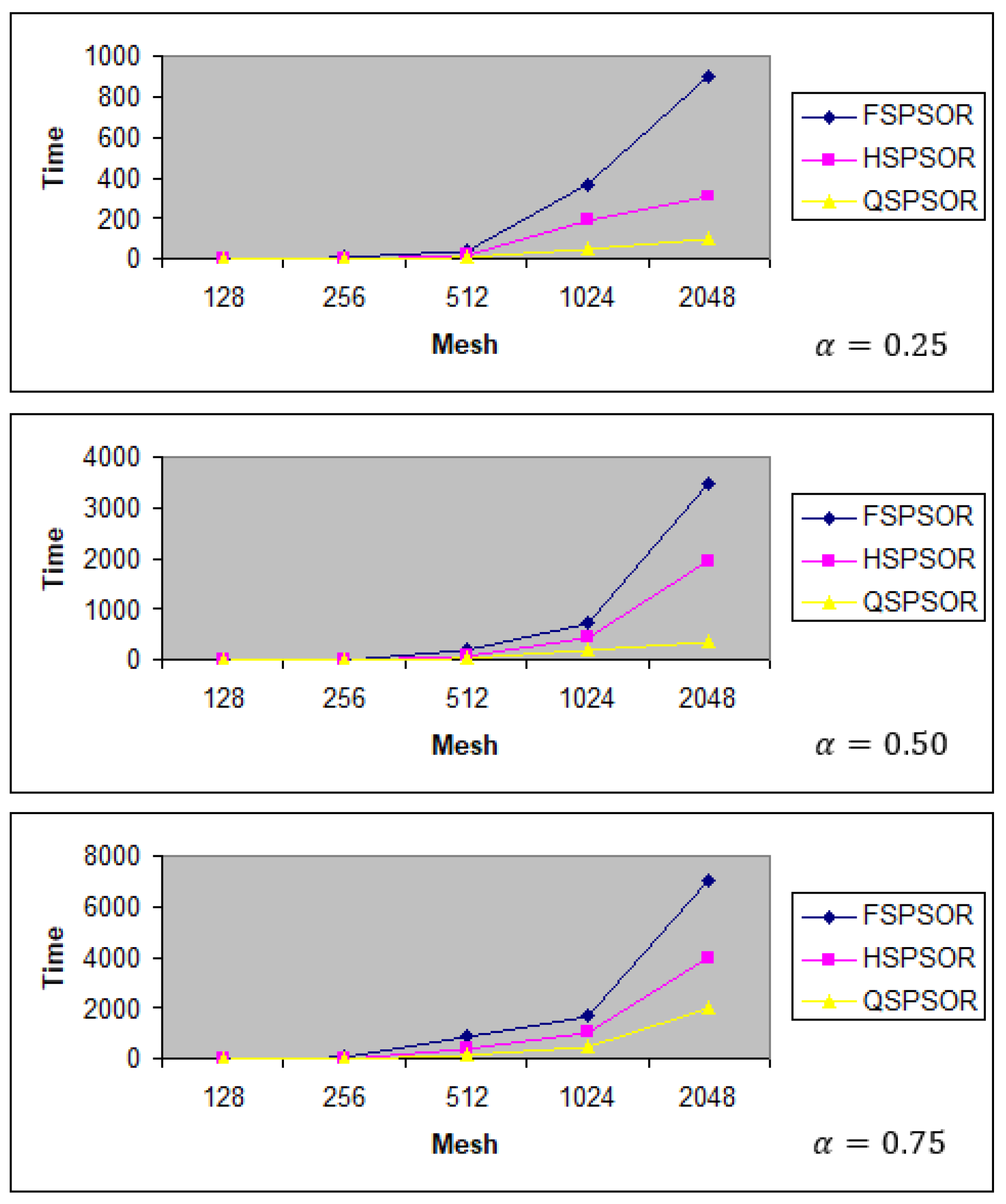
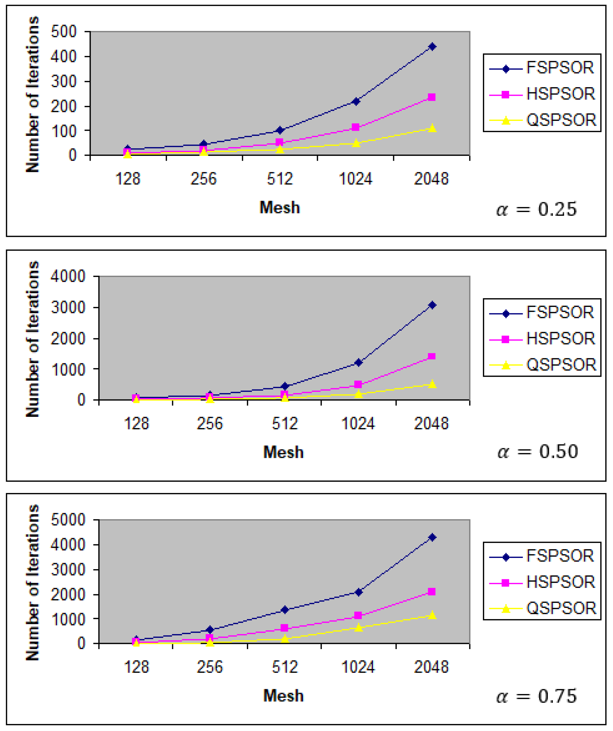
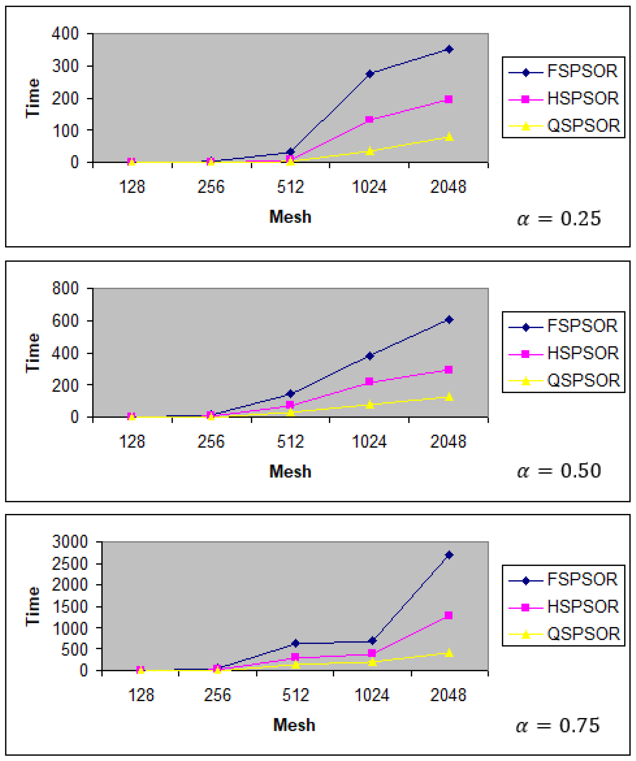
  • The QSPSOR method significantly reduced the number of iterations and execution time compared to the existing FSPSOR and HSPSOR methods. On average, QSPSOR reduced the number of iterations and execution time by 81.19% and 84.06%, respectively, compared to FSPSOR. Moreover, QSPSOR reduced the number of iterations and execution time compared to HSPSOR by 59.94% and 66.00%, respectively. The result also showed that using the quarter-sweep scheme and PSOR iteration can reduce the computational complexity for solving the time FDE with a large matrix size.
  • Observations regarding the accuracy of all of the implemented numerical methods indicated that their numerical solutions were in good agreement. Furthermore, the accuracy of the solutions of the time-FDE problems obtained by each of the three numerical methods was greater at α = 0.50 , followed by α = 0.75 and α = 0.25 . The combination of the quarter-sweep implicit finite difference scheme and Caputo’s time-fractional derivative enabled an accurate solution for the time FDE to be computed.
  • However, a disadvantage of the quarter-sweep difference scheme is that the magnitude of the absolute errors is slightly larger than that of the two previous methods. The accuracy of the quarter-sweep scheme can be improved by applying a suitable treatment.
Thus, the combination of a quarter-sweep finite difference method, Caputo’s time-fractional derivative, and the preconditioned successive over-relaxation method showed good potential to solve different types of fractional mathematical equations, and provides a future direction for this field of research.

Author Contributions

Writing—original draft preparation, A.S.; writing—review and editing, J.V.L.C.; supervision, P.A., J.S. and S.M. All authors have read and agreed to the published version of the manuscript.

Funding

This research received no external funding.

Institutional Review Board Statement

Not applicable.

Informed Consent Statement

Not applicable.

Data Availability Statement

Not applicable.

Conflicts of Interest

The authors declare no conflict of interest.

References

  1. Sweilam, N.; Kareem, W.A.; Al-Mekhlafi, S.; Nabih, Z. Numerical treatments for a complex order fractional HIV infection model with drug resistance during therapy. Prog. Fract. Differ. Appl. 2021, 7, 163–176. [Google Scholar] [CrossRef]
  2. Alrabaiah, H.; Zeb, A.; Alzahrani, E.; Shah, K. Dynamical analysis of fractional-order tobacco smoking model containing snuffing class. Alex. Eng. J. 2021, 60, 3669–3678. [Google Scholar] [CrossRef]
  3. Wang, X.; Qi, H.; Yang, X.; Xu, H. Analysis of the time-space fractional bioheat transfer equation for biological tissues during laser irradiation. Int. J. Heat Mass Transf. 2021, 177, 121555. [Google Scholar] [CrossRef]
  4. Moosavi, R.; Moltafet, R.; Shekari, Y. Analysis of viscoelastic non-Newtonian fluid over a vertical forward-facing step using the Maxwell fractional model. Appl. Math. Comput. 2021, 401, 126119. [Google Scholar] [CrossRef]
  5. Gu, X.-M.; Sun, H.-W.; Zhao, Y.-L.; Zheng, X. An implicit difference scheme for time-fractional diffusion equations with a time-invariant type variable order. Appl. Math. Lett. 2021, 120, 107270. [Google Scholar] [CrossRef]
  6. Davis, W.; Noren, R.; Shi, K. A Cα finite difference method for the Caputo time-fractional diffusion equation. Numer. Methods Part. Differ. Equ. 2021, 37, 2261–2277. [Google Scholar] [CrossRef]
  7. Hosseininia, M.; Heydari, M.H.; Maalek Ghaini, F.M. A numerical method for variable-order fractional version of the coupled 2D Burgers equations by the 2D Chelyshkov polynomials. Math. Methods Appl. Sci. 2021, 44, 6482–6499. [Google Scholar] [CrossRef]
  8. Mirzaee, F.; Sayevand, K.; Rezaei, S.; Samadyar, N. Finite difference and spline approximation for solving fractional stochastic advection-diffusion equation. Iran. J. Sci. Technol. Trans. A Sci. 2021, 45, 607–617. [Google Scholar] [CrossRef]
  9. González-Olvera, M.A.; Torres, L.; Hernández-Fontes, J.V.; Mendoza, E. Time fractional diffusion equation for shipping water events simulation. Chaos Solitons Fractals 2021, 143, 110538. [Google Scholar] [CrossRef]
  10. Liao, X.; Feng, M. Time-fractional diffusion equation-based image denoising model. Nonlinear Dyn. 2021, 103, 1999–2017. [Google Scholar] [CrossRef]
  11. Maldon, B.; Thamwattana, N. A fractional diffusion model for dye-sensitized solar cells. Molecules 2020, 25, 2966. [Google Scholar] [CrossRef] [PubMed]
  12. Bohaienko, V.; Bulavatsky, V. Simplified mathematical model for the description of anomalous migration of soluble substances in vertical filtration flow. Fractal Fract. 2020, 4, 20. [Google Scholar] [CrossRef]
  13. Li, L.; Jiang, Z.; Yin, Z. Compact finite-difference method for 2D time-fractional convection–diffusion equation of groundwater pollution problems. Comput. Appl. Math. 2020, 39, 142. [Google Scholar] [CrossRef]
  14. Aguilar, J.-P.; Korbel, J.; Luchko, Y. Applications of the fractional diffusion equation to option pricing and risk calculations. Mathematics 2019, 7, 796. [Google Scholar] [CrossRef] [Green Version]
  15. Li, Y.; Liu, F.; Turner, I.W.; Li, T. Time-fractional diffusion equation for signal smoothing. Appl. Math. Comput. 2018, 326, 108–116. [Google Scholar] [CrossRef] [Green Version]
  16. Sunarto, A.; Sulaiman, J. Preconditioned SOR method to solve time-fractional diffusion equations. J. Phys. Conf. Ser. 2019, 1179, 012020. [Google Scholar] [CrossRef]
  17. Sunarto, A.; Sulaiman, J. Application half-sweep preconditioned SOR method for solving time-fractional diffusion equations. In Proceedings of the International Conference on Industrial Engineering and Operations Management, Detroit, MI, USA, 10–14 August 2020; pp. 3414–3420. [Google Scholar]
  18. Lung, J.C.V.; Sulaiman, J. On quarter-sweep finite difference scheme for one-dimensional porous medium equations. Int. J. Appl. Math. 2020, 33, 439–450. [Google Scholar] [CrossRef]
  19. Muhiddin, F.A.; Sulaiman, J.; Sunarto, A. Numerical evaluation of quarter-sweep KSOR method to solve time-fractional parabolic equations. Int. J. Eng. Trends Technol. 2020, 2020, 63–69. [Google Scholar] [CrossRef]
  20. Suardi, M.N.; Radzuan, N.Z.F.M.; Sulaiman, J. Performance analysis of quarter-sweep Gauss-Seidel iteration with cubic B-spline approach to solve two-point boundary value problems. Adv. Sci. Lett. 2018, 24, 1732–1735. [Google Scholar] [CrossRef]
  21. Atangana, A. Fractional Operators and Their Applications. In Fractional Operators with Constant and Variable Order with Application to Geo-Hydrology; Atangana, A., Ed.; Academic Press: Cambridge, MA, USA, 2018; Chapter 5; pp. 79–112. [Google Scholar]
  22. Demir, A.; Erman, S.; Özgür, B.; Korkmaz, E. Analysis of fractional partial differential equations by Taylor series expansion. Bound. Value Probl. 2013, 2013, 68. [Google Scholar] [CrossRef] [Green Version]
Figure 1. Graphs of performance of FSPSOR, HSPSOR, and QSPSOR methods to solve Example 1, showing mesh sizes versus number of iterations for three different fractional orders.
Fractalfract 05 00098 g001
Figure 2. Graphs of performance of FSPSOR, HSPSOR, and QSPSOR methods to solve Example 1, showing mesh sizes versus execution time for three different fractional orders.
Fractalfract 05 00098 g002
Figure 3. Graphs of performance of FSPSOR, HSPSOR, and QSPSOR methods to solve Example 2, showing mesh sizes versus number of iterations at three different fractional orders.
Fractalfract 05 00098 g003
Figure 4. Graphs of performance of FSPSOR, HSPSOR, and QSPSOR methods to solve Example 2, showing mesh sizes versus execution time at three different fractional orders.
Fractalfract 05 00098 g004
Table 1. QSPSOR computational algorithm.
Set   ψ ( 0 ) = 0 and the Tolerance Error ε = 10 10 .
(i) For   n = 1 , 2 , , N and for i = 4 ,   8 , , M 4 , iterate the formula shown in Equation (43),
(ii) Compute   Z ˜ ( η + 1 ) = P T ψ ( η + 1 ) ,
(iii) Convergence   criterion   Z ˜ ( η + 1 ) Z ˜ ( η ) < ε ,
(iv)If the criterion is achieved, display approximate solutions.
Table 2. Comparison between FSPSOR, HSPSOR, and QSPSOR in solving Example 1.
M Method α = 0.25 α = 0.50 α = 0.75
η s e c . ε ^ η s e c . ε ^ η s e c . ε ^
128FSPSOR280.842.36 × 102801.906.20 × 1042465.763.99 × 102
HSPSOR160.182.36 × 102370.546.99 × 104942.363.99 × 102
QSPSOR80.052.37 × 102140.296.19 × 104320.094.21 × 102
256FSPSOR535.332.43 × 10221117.845.69 × 10480667.753.97 × 102
HSPSOR342.202.43 × 102946.906.21 × 10430334.653.97 × 102
QSPSOR150.272.44 × 102392.376.99 × 10410112.844.03 × 102
512FSPSOR12041.432.46 × 102566182.835.36 × 1042635843.913.96 × 102
HSPSOR6721.652.46 × 10224686.095.36 × 104988421.583.96 × 102
QSPSOR315.042.47 × 10210040.616.21 × 104337198.203.96 × 102
1024FSPSOR250372.352.48 × 1021514726.295.13 × 10460121699.873.95 × 102
HSPSOR141189.582.48 × 102655434.725.13 × 10424131003.783.95 × 102
QSPSOR6647.292.49 × 102266214.515.69 × 1041095501.763.95 × 102
2048FSPSOR808901.762.49 × 10240523469.735.13 × 10435,2897052.283.93 × 102
HSPSOR305308.802.49 × 10217881956.435.13 × 10418,1434025.903.93 × 102
QSPSOR14395.252.50 × 102709365.435.35 × 10435742000.833.93 × 102
Table 3. Comparison between FSPSOR, HSPSOR, and QSPSOR in solving Example 2.
M Method α = 0.25 α = 0.50 α = 0.75
η s e c . ε ^ η s e c . ε ^ η s e c . ε ^
128FSPSOR280.842.36 × 102801.906.20 × 1042465.763.99 × 102
HSPSOR160.182.36 × 102370.546.99 × 104942.363.99 × 102
QSPSOR80.052.37 × 102140.296.19 × 104320.094.21 × 102
256FSPSOR535.332.43 × 10221117.845.69 × 10480667.753.97 × 102
HSPSOR342.202.43 × 102946.906.21 × 10430334.653.97 × 102
QSPSOR150.272.44 × 102392.376.99 × 10410112.844.03 × 102
512FSPSOR12041.432.46 × 102566182.835.36 × 1042635843.913.96 × 102
HSPSOR6721.652.46 × 10224686.095.36 × 104988421.583.96 × 102
QSPSOR315.042.47 × 10210040.616.21 × 104337198.203.96 × 102
1024FSPSOR250372.352.48 × 1021514726.295.13 × 10460121699.873.95 × 102
HSPSOR141189.582.48 × 102655434.725.13 × 10424131003.783.95 × 102
QSPSOR6647.292.49 × 102266214.515.69 × 1041095501.763.95 × 102
2048FSPSOR808901.762.49 × 10240523469.735.13 × 10435,2897052.283.93 × 102
HSPSOR305308.802.49 × 10217881956.435.13 × 10418,1434025.903.93 × 102
QSPSOR14395.252.50 × 102709365.435.35 × 10435742000.833.93 × 102
Publisher’s Note: MDPI stays neutral with regard to jurisdictional claims in published maps and institutional affiliations.

