Design, Convergence and Stability of a Fourth-Order Class of Iterative Methods for Solving Nonlinear Vectorial Problems

Abstract

A new parametric family of iterative schemes for solving nonlinear systems is presented. Fourth-order convergence is demonstrated and its stability is analyzed as a function of the parameter values. This study allows us to detect the most stable elements of the class, to find the fractals in the boundary of the basins of attraction and to reject those with chaotic behavior. Some numerical tests show the performance of the new methods, confirm the theoretical results and allow to compare the proposed schemes with other known ones.

1. Introduction

To find the solutions $\overline{z}$ of systems of nonlinear equations $F\left(z\right)=0$, where $F:D\subseteq {\mathbb{R}}^n\to {\mathbb{R}}^n$ is a real vectorial function of several variables, is a classical and important problem in Science and Engineering. There are no analytical methods to find the solutions to these problems, so we must use iterative schemes that approximate them.

The most known algorithm in this context is classical Newton’s scheme, expressed as

$$z^{(i+1)}=z^{\left(i\right)}-{\left[F^{\prime }\left(z^{\left(i\right)}\right)\right]}^{-1}F\left(z^{\left(i\right)}\right),i=0,1,\dots ,$$

where $F^{\prime }$ represents the Jacobian matrix associated to function F. This scheme has quadratic convergence under some conditions of F, $F^{\prime }$ and the initial estimation $z^{\left(0\right)}$.

Different techniques can be used in order to design Newton-like iterative schemes, as direct composition, weight functions, estimations of $F^{\prime }\left(z\right)$ by means of the divided difference operator, etc. So, some high-order methods for computing the solutions of $F\left(z\right)=0$ have been proposed in the literature. These new schemes are proposed with the aim of accelerating the convergence or improving the computational efficiency. For example, recently the authors proposed in [1,2,3] new parametric families of iterative methods and a fast algorithm for solving nonlinear systems. Other researchers have published iterative methods that avoid the Jacobian matrix with interesting orders of convergence, see, for instance [4,5,6]. In these manuscripts the Jacobian matrix is replaced by $[·,·;F]$, the divided difference operator.

The procedure of weight functions (in this case, matrix functions) plays also an important role for designing schemes for solving systems $F\left(z\right)=0$, as we can see in [7,8]. Iterative processes with memory for systems are also beginning to appear in the literature. These are methods in which the new iteration is obtained from at least the previous two. In general, the convergence order is increased without adding functional evaluations [9,10,11].

In [12] the authors presented a class of iterative schemes depending on a parameter, whose iterative expression is

$$\begin{array}{ccc}\hfill y^{\left(i\right)}& =& z^{\left(i\right)}-{\left[F^{\prime }\left(z^{\left(i\right)}\right)\right]}^{-1}F\left(z^{\left(i\right)}\right),\hfill \\ \hfill u^{\left(i\right)}& =& y^{\left(i\right)}-\frac{1}{\beta }{\left[F^{\prime }\left(z^{\left(i\right)}\right)\right]}^{-1}F\left(y^{\left(i\right)}\right),\hfill \\ \hfill z^{(i+1)}& =& z^{\left(i\right)}-{\left[F^{\prime }\left(z^{\left(i\right)}\right)\right]}^{-1}\left[(2-1/\beta -\beta )F\left(y^{\left(i\right)}\right)+\beta F\left(u^{\left(i\right)}\right)\right],i=0,1,\dots ,\hfill \end{array}$$

(1)

where $\beta \ne 0$ is a real parameter. Let us observe that, for each iteration, we only need an inverse operator, so the three linear systems that we need to solve in each iteration have the same matrix of coefficient and therefore the number of operations (products and quotients) is reduced. For any value of the parameter, these schemes have order of convergence four and, in particular, for $\beta =1/5$ we reach order five. This particular case was used in [13] for determining preliminary orbits of artificial satellites. Family (1) is denoted by $M4\left(\beta \right)$.

Now, we are going to recall some concepts used to prove the order of convergence, some of them firstly introduced in [14].

Let us consider a sequence ${\left\{z^{\left(i\right)}\right\}}_{i\ge 0}$ in ${\mathbb{R}}^n$, converging to $\overline{z}$. Then, it has order of convergence p, $p\ge 1$, if there exists $K>0$, ($0<K<1$ if $p=1$), and $i_0$ such that

$$\parallel z^{(i+1)}-\overline{z}\parallel \le K\parallel z^{\left(i\right)}-\overline{z}{\parallel }^p,\forall i\ge i_0,$$

or

$$\parallel e^{(i+1)}\parallel \le K\parallel e^{\left(i\right)}{\parallel }^p,\forall i\ge i_0,$$

being $e^{\left(i\right)}=z^{\left(i\right)}-\overline{z}$, $i=0,1,2,\dots$

To present a rigorous proof of the order of convergence of a vectorial iterative method, we introduced in [14] the following notation which we now recall for completeness.

Let $F:D\subseteq {\mathbb{R}}^n⟶{\mathbb{R}}^n$ be a sufficiently Fréchet differentiable function in set D, that must be open and convex. The qth derivative of F at $v\in {\mathbb{R}}^n$, $q\ge 1$, is the q-linear function

$$F^{\left(q\right)}\left(v\right):{\mathbb{R}}^n\times \cdots \times {\mathbb{R}}^n⟶{\mathbb{R}}^n,\mathrm{such}\mathrm{that}{F}^{\left(q\right)}\left(v\right)(u_1,\dots ,u_q)\in {\mathbb{R}}^n.$$

For $q=1$, $F^{\prime }\left(v\right)$ is the Jacobian matrix evaluated in v, that is, a linear operator $F^{\prime }\left(v\right):{\mathbb{R}}^n⟶{\mathbb{R}}^n$, such that $F^{\prime }\left(v\right)\left(u\right)=F^{\prime }\left(v\right)u$. Let us remark that

(1)

$F^{\left(q\right)}\left(v\right)(u_1,\dots ,u_{q-1},·)\in \mathcal{L}\left({\mathbb{R}}^n\right)$, where $\mathcal{L}\left({\mathbb{R}}^n\right)$ is the set of linear operators in ${\mathbb{R}}^n$.

(2)

$F^{\left(q\right)}\left(v\right)(u_{\sigma \left(1\right)},\dots ,u_{\sigma \left(q\right)})=F^{\left(q\right)}\left(v\right)(u_1,\dots ,u_q)$, being $\sigma$ any permutation of $\{1,2,\dots ,q\}$.

From (1) and (2), we recall the notation:

(i)

$F^{\left(q\right)}\left(v\right)(u_1,\dots ,u_q)=F^{\left(q\right)}\left(v\right)u_1\dots u_q$,

(ii)

$F^{\left(p\right)}\left(v\right)u^{p-1}{F}^{\left(q\right)}{u}^q=F^{\left(p\right)}\left(v\right)F^{\left(q\right)}\left(v\right)u^{q-1+p}$.

Moreover, let $\overline{z}+h\in {\mathbb{R}}^n$ lie in a neighborhood of $\overline{z}$, $F\left(\overline{z}\right)=0$. By applying Taylor expansion around $\overline{z}$ and assuming that $F^{\prime }\left(\overline{z}\right)$ is nonsingular,

$$F(\overline{z}+h)=F^{\prime }\left(\overline{z}\right)\left[h+\sum _{k=2}^{p-1}{C}_k{h}^k\right]+\mathcal{O}\left(h^p\right),$$

(2)

being $C_k={\displaystyle \frac{1}{k!}}{\left[F^{\prime }\left(\overline{z}\right)\right]}^{-1}{F}^{\left(k\right)}\left(\overline{z}\right)\in {\mathbb{R}}^n$, $k\ge 2$.

In addition, we can describe the Taylor expansion of $F^{\prime }$ around $\overline{z}$ as

$$F^{\prime }(\overline{z}+h)=F^{\prime }\left(\overline{z}\right)\left[I+\sum _{q=2}^{p-1}q{C}_q{h}^{q-1}\right]+\mathcal{O}\left(h^{p-1}\right),$$

(3)

where I is the identity matrix of size $n\times n$. Therefore, $q{C}_q{h}^{q-1}\in \mathcal{L}\left({\mathbb{R}}^n\right)$. From (3), we conjecture

$${\left[F^{\prime }(\overline{z}+h)\right]}^{-1}=\left[I+A_{2}h+A_3{h}^2+A_4{h}^4+\cdots \right]{\left[F^{\prime }\left(\overline{z}\right)\right]}^{-1}+\mathcal{O}\left(h^{p-1}\right),$$

(4)

where $A_j$, $j=2,3,\dots$, are obtained by forcing that $\left[F^{\prime }(\overline{z}+h)\right]{\left[F^{\prime }(\overline{z}+h)\right]}^{-1}=I$, which gives

$$\begin{array}{ccc}\hfill A_2& =& -2C_2,\hfill \\ \hfill A_3& =& 4C_2^2-3C_3,\hfill \\ \hfill A_4& =& -8C_2^3+6C_2{C}_3+6C_3{C}_2-4C_4,\hfill \\ & ⋮\end{array}$$

The equation

$$e^{(i+1)}=L{e^{\left(i\right)}}^p+\mathcal{O}\left({e^{\left(i\right)}}^{p+1}\right),$$

where p is the order of convergence and L is a p-linear operator, is called the error equation and we consider ${e^{\left(i\right)}}^p=(e^{\left(i\right)},e^{\left(i\right)},\dots ,e^{\left(i\right)})$.

We summarize the contents of this manuscript: the new class of iterative methods for solving nonlinear systems is presented in Section 2, and its convergence is analyzed. As all the methods of the class have the same order, their qualitative properties are under study in Section 3. Section 4 is devoted to numerical tests for confirming the theoretical results and also show how the new schemes perform. This manuscript ends with some conclusions.

2. Construction and Analysis of the Methods

From damped Newton’s method and following the ideas presented by Sharma and Arora in [15], we propose the following parametric class of multipoint schemes for approximating the solutions of nonlinear systems, whose iterative expression is

$$\begin{array}{cc}\hfill y^{\left(i\right)}& =z^{\left(i\right)}-\alpha {\left[F^{\prime }\left(z^{\left(i\right)}\right)\right]}^{-1}F\left(z^{\left(i\right)}\right),\hfill \\ \hfill z^{(i+1)}& =z^{\left(i\right)}-(\beta {\left[F^{\prime }\left(y^{\left(i\right)}\right)\right]}^{-1}{F}^{\prime }\left(z^{\left(i\right)}\right){\left[F^{\prime }\left(y^{\left(i\right)}\right)\right]}^{-1}+\gamma {\left[F^{\prime }\left(y^{\left(i\right)}\right)\right]}^{-1}+\mu {\left[F^{\prime }\left(z^{\left(i\right)}\right)\right]}^{-1}\hfill \\ \hfill & \phantom{=}+\delta {\left[F^{\prime }\left(z^{\left(i\right)}\right)\right]}^{-1}{F}^{\prime }\left(y^{\left(i\right)}\right){\left[F^{\prime }\left(z^{\left(i\right)}\right)\right]}^{-1})F\left(z^{\left(i\right)}\right),i=0,1,\dots ,\hfill \end{array}$$

(5)

where $\alpha ,\beta ,\gamma ,\mu ,\delta$ are real parameters to be chosen to obtain the highest order of convergence. In what follows, we fix the conditions for this convergence.

Theorem 1.

Let $F:D\subseteq {\mathbb{R}}^n⟶{\mathbb{R}}^n$ be sufficiently differentiable at its open convex domain D. Let also $\overline{z}\in {\mathbb{R}}^n$ be a solution of $F\left(z\right)=0$ and let us assume that $z^{\left(0\right)}$ is close enough to $\overline{z}$. Supposing $F^{\prime }\left(z\right)$ to be nonsingular and continuous at $\overline{z}$, sequence ${\left\{z^{\left(i\right)}\right\}}_{i\ge 0}$ obtained from (5) converges to $\overline{z}$ with fourth-order for ${\displaystyle \alpha =\frac{2}{3}}$, ${\displaystyle \beta =\frac{3}{8}-\frac{\gamma }{3}}$, ${\displaystyle \mu =\frac{5}{8}-\gamma }$, ${\displaystyle \delta =\frac{\gamma }{3}}$, being γ a free disposable parameter. In this case, the error equation is

$$e^{(i+1)}=\left(-\frac{117+64\gamma }{81}{C}_2^3-\frac{1}{9}{C}_4+\frac{9-8\gamma }{18}{C}_2{C}_3+\frac{9+8\gamma }{18}{C}_3{C}_2\right){e^{\left(i\right)}}^4+\mathcal{O}\left({e^{\left(i\right)}}^5\right),$$

where $C_q={\displaystyle \frac{1}{q!}}{\left[F^{\prime }\left(\overline{z}\right)\right]}^{-1}{F}^{\left(q\right)}\left(\overline{z}\right)$, $q=2,3,\dots$ and $e^{\left(i\right)}=z^{\left(i\right)}-\overline{z}.$

Proof. 

Let us consider the Taylor expansion of $F\left(z^{\left(i\right)}\right)$, and its derivative around $\overline{z}$. Then, we have

$${\left[F^{\prime }\left(z^{\left(i\right)}\right)\right]}^{-1}=\left(I+A_2{e}^{\left(i\right)}+A_3{e^{\left(i\right)}}^2+A_4{e^{\left(i\right)}}^3+A_5{e^{\left(i\right)}}^4\right){\left[F^{\prime }\left(\overline{z}\right)\right]}^{-1}+\mathcal{O}\left({e^{\left(i\right)}}^5\right),$$

where

$$\begin{array}{cc}\hfill A_2& =-2C_2,\hfill \\ \hfill A_3& =-3C_3+4C_2^2,\hfill \\ \hfill A_4& =-4C_4+6C_2{C}_3+6C_3{C}_2-8C_2^3,\hfill \end{array}$$

and

$$\begin{array}{cc}\hfill {\left[F^{\prime }\left(z^{\left(i\right)}\right)\right]}^{-1}F\left(z^{\left(i\right)}\right)& =e^{\left(i\right)}-C_2{e^{\left(i\right)}}^2+2(C_2^2-C_3){e^{\left(i\right)}}^3\hfill \\ & +(4C_2{C}_3+3C_3{C}_2-3C_4-4C_2^3){e^{\left(i\right)}}^4+\mathcal{O}\left({e^{\left(i\right)}}^5\right).\hfill \end{array}$$

So,

$$\begin{array}{cc}\hfill y^{\left(i\right)}-\overline{z}& =(1-\alpha )e^{\left(i\right)}+\alpha C_2{e^{\left(i\right)}}^2-2\alpha (-C_3+C_2^2){e^{\left(i\right)}}^3+\mathcal{O}\left({e^{\left(i\right)}}^4\right),\hfill \\ \hfill {(y^{\left(i\right)}-\overline{z})}^2& ={(1-\alpha )}^2{e^{\left(i\right)}}^2+2\alpha (1-\alpha )C_2{e^{\left(i\right)}}^3+\mathcal{O}\left({e^{\left(i\right)}}^4\right),\hfill \\ \hfill {(y^{\left(i\right)}-\overline{z})}^3& ={(1-\alpha )}^3{e^{\left(i\right)}}^3+\mathcal{O}\left({e^{\left(i\right)}}^4\right),\hfill \end{array}$$

and

$$\begin{array}{ccc}\hfill F^{\prime }\left(y^{\left(i\right)}\right)& =& F^{\prime }\left(\overline{z}\right)\left(I+2C_2(y^{\left(i\right)}-\overline{z})+3C_3{(y^{\left(i\right)}-\overline{z})}^2+4C_4{(y^{\left(i\right)}-\overline{z})}^3\right)+\mathcal{O}\left({(y^{\left(i\right)}-\overline{z})}^4\right)\hfill \end{array}$$

(6)

$$\begin{array}{ccc}& =& F^{\prime }\left(\overline{z}\right)(I+2(1-\alpha )C_2{e}^{\left(i\right)}+(3{(1-\alpha )}^2{C}_3+2\alpha C_2^2){e^{\left(i\right)}}^2\hfill \end{array}$$

(7)

$$\begin{array}{ccc}& & +(4{(1-\alpha )}^3{C}_4-4\alpha C_2^3+6\alpha (1-\alpha )C_3{C}_2+4\alpha C_2{C}_3){e^{\left(i\right)}}^3)+\mathcal{O}\left({e^{\left(i\right)}}^4\right).\hfill \end{array}$$

(8)

Therefore,

$${\left[F^{\prime }\left(y^{\left(i\right)}\right)\right]}^{-1}=\left(I+Y_2{e}^{\left(i\right)}+Y_3{e^{\left(i\right)}}^2\right){\left[F^{\prime }\left(\overline{z}\right)\right]}^{-1}+\mathcal{O}\left({e^{\left(i\right)}}^4\right),$$

(9)

where

$$\begin{array}{cc}\hfill Y_2& =-2(1-\alpha )C_2,\hfill \\ \hfill Y_3& =-3{(1-\alpha )}^2{C}_3+2(2{\alpha }^2-5\alpha +2)C_2^2.\hfill \end{array}$$

Then, by replacing the development of $F\left(z^{\left(i\right)}\right)$ and (9) in the second step of the iterative expression, we get the error equation

$$\begin{array}{cc}\hfill e^{(i+1)}& =(1-\beta -\gamma -\mu -\delta )e^{\left(i\right)}-(4\alpha \beta -\beta -\gamma +2\alpha \gamma -\mu -2\alpha \delta )C_2{e^{\left(i\right)}}^2\hfill \\ & \phantom{=}-((12{\alpha }^2\beta -16\alpha \beta +2\beta +4{\alpha }^2\gamma -8\alpha \gamma +2\gamma +2\mu +2\delta +18\alpha \delta )C_2^2\hfill \\ & \phantom{=}+(-6{\alpha }^2\beta +12\alpha \beta -2\beta -3{\alpha }^2\gamma +6\alpha \gamma -2\gamma -2\mu +3{\alpha }^2\delta -6\alpha \delta -2\delta )C_3){e^{\left(i\right)}}^3+\mathcal{O}\left({e^{\left(i\right)}}^4\right).\hfill \end{array}$$

So, in order to get the desired order four, the following equations must be satisfied,

$$\begin{array}{cc}\hfill 0& =1-\beta -\gamma -\mu -\delta ,\hfill \\ \hfill 0& =-\beta -\gamma -\mu +2\alpha (\gamma +2\beta -\delta ),\hfill \\ \hfill 0& =2(\beta +\gamma +\mu +\delta )+12{\alpha }^2\beta -16\alpha \beta +4{\alpha }^2\gamma -8\alpha \gamma +18\alpha \delta ,\hfill \\ \hfill 0& =-2(\beta +\gamma +\mu +\delta )-6{\alpha }^2\beta +12\alpha \beta -3{\alpha }^2\gamma +6\alpha \gamma +3{\alpha }^2\delta -6\alpha \delta .\hfill \end{array}$$

The solutions of this system are $\alpha ={\displaystyle \frac{2}{3}},$${\displaystyle \beta =\frac{3}{8}-\frac{\gamma }{3},}$${\displaystyle \mu =\frac{5}{8}-\gamma }$, ${\displaystyle \delta =\frac{\gamma }{3}}$, where $\gamma$ is a disposable parameter. Then,

$$e^{(i+1)}=\left(-\frac{117+64\gamma }{81}{C}_2^3+\frac{9-8\gamma }{18}{C}_2{C}_3+\frac{9+8\gamma }{18}{C}_3{C}_2-\frac{C_4}{9}\right){e^{\left(i\right)}}^4+\mathcal{O}\left({e^{\left(i\right)}}^5\right),$$

and the fourth-order of convergence is proven. □

We denote this uniparametric class of iterative methods by PM4$\left(\gamma \right)$. Some particular values of $\gamma$ can yield to simpler iterative expressions, as in case of $\gamma =\frac{9}{8}$ that coincides with Sharma et al. scheme, that was proposed in [8]. In the following section we discuss, by using discrete dynamics, which elements of this family have better qualitative properties.

3. Stability Analysis of Class PM4$\left(\mathbf{\gamma }\right)$

The qualitative performance of the vectorial rational operator related to an iterative method applied to a low-degree polynomial system has demonstrated to be a useful and efficient tool for the study of the stability of the methods, see for example [16,17,18,19] and the references therein.

Now, our aim is to determine which elements of class of iterative methods PM4$\left(\gamma \right)$ present low dependence of the convergence regarding the starting guess used. To get this aim, let us recall some basic definitions of the real multidimensional discrete dynamics tools.

Let us consider $R\left(z\right)$ as the rational fixed-point vectorial function associated to a family of methods acting on a polynomial system $p\left(z\right)=0$ with n variables, $p:{\mathbb{R}}^n\to {\mathbb{R}}^n$. Many of the following concepts are direct extension of their partners in complex dynamics [16,20].

The orbit of $z^{\left(0\right)}\in {\mathbb{R}}^n$ is defined as $\left\{z^{\left(0\right)},R\left(z^{\left(0\right)}\right),\dots ,R^m\left(z^{\left(0\right)}\right),\dots \right\}$. A point $z^{*}\in {\mathbb{R}}^n$ is a fixed point of R if $R\left(z^{*}\right)=z^{*}$, and it is called strange fixed point when it is not a root of $p\left(z\right)=0$. The stability of the fixed points is characterized by Robinson [20]. He states the character of a k-periodic point $z^{*}$ depending on the eigenvalues of $R^{\prime }\left(z^{*}\right)$, ${\lambda }_1,{\lambda }_1,\dots ,{\lambda }_n$. It is repelling if all $|{\lambda }_j|>1$, $j=1,2,\dots ,n$, unstable or saddle if at least one $j_0$ exists such that $|{\lambda }_{j_0}|>1$ and attracting if all $|{\lambda }_j|<1$, $j=1,2,\dots ,n$. In addition, a fixed point is called hyperbolic if ${\lambda }_j$ satisfies $|{\lambda }_j|\ne 1$, for all j.

In the following, we denote by $Op4(z,\gamma )=(o_1^4(z,\gamma ),o_2^4(z,\gamma ),\dots ,o_n^4(z,\gamma ))$, the fixed point function associated to (5) class, applied on n-dimensional quadratic polynomial system $p\left(z\right)=0$, where:

$$\begin{array}{c}{p}_i\left(z\right)=z_i^2-1,i=1,2,\dots ,n.\hfill \end{array}$$

(10)

Coordinate functions $o_j^4(z,\gamma )$ differ only in the sub-index $j=1,2,\dots ,n$. These coordinate functions of $Op4(z,\gamma )$ are expressed as -4.6cm0cm

$$o_j^4(z,\gamma )=\frac{8\gamma +8\gamma z_j^8+153z_j^8-32\gamma z_j^6+819z_j^6+48\gamma z_j^4+279z_j^4-32\gamma z_j^2+45z_j^2}{144z_j^3{\left(2z_j^2+1\right)}^2},\mathrm{for} j=1,2,\dots ,n.$$

(11)

The stability analysis of the fixed points of $Op4(z,\gamma )$ is presented in the following result.

Theorem 2.

Rational operator $Op4(z,\gamma )$ corresponding to PM4$\left(\gamma \right)$ has $2^n$ fixed points, that are superattracting, whose components are zeros of polynomial system $p\left(z\right)$. This operator also has a different number of real strange fixed points whose components are combination of the real roots of

$$q\left(t\right)=t^6(8\gamma -423)+t^4(-24\gamma -180)+t^2(24\gamma -45)-8\gamma ,$$

depending on γ, denoted by$q_1\left(\gamma \right)$and$q_2\left(\gamma \right)$(being the only ones that are real, if any), and the roots of$p\left(z\right)$:

(a)

If$\gamma <0$or$\gamma >{\displaystyle \frac{423}{8}}$, the roots$q_i\left(\gamma \right)$, $i=1,2$, are real. Then, the strange fixed points expressed as$(q_{{\sigma }_1}\left(\gamma \right),q_{{\sigma }_2}\left(\gamma \right),\dots ,q_{{\sigma }_n}\left(\gamma \right))$being${\sigma }_i\in \{1,2\}$, are repelling. Moreover, if at least one (but not all) component of an strange fixed point is equal to$\pm 1$, then it is saddle.

(b)

If$0<\gamma <{\displaystyle \frac{423}{8}}$, then the roots of$q\left(t\right)$are not real. So, do not exist strange fixed points.

Proof. 

In order to calculate the fixed points of $Op4(z,\gamma )$, we solve $o_j^4(z,\gamma )=z_j$,

$$-(z_j^2-1)\frac{-8\gamma +(8\gamma -423)z_j^6-12(2\gamma +15)z_j^4+3(8\gamma -15)z_j^2}{144z_1^3{\left(2z_1^2+1\right)}^2}=0,$$

for $j=1,2,\dots ,n$. Then, $z_j=\pm 1$ are components of the fixed points and also are ($q_i\left(\gamma \right)$, $i=1,2,\dots ,6$), being $t\ne 0$.

Depending on $\gamma$, at most two roots of $q\left(t\right)$ are real. The, the eigenvalues of $Op{4}^{\prime }(z,\gamma )$ can be expressed as

$$\begin{array}{ccc}\hfill Ei{g}_j(z_1\left(\gamma \right),\dots ,z_n\left(\gamma \right))& =& \frac{{\left(z_j^2-1\right)}^3\left(24\gamma +16\gamma z_j^4+306z_j^4+152\gamma z_j^2+45z_j^2\right)}{144z_j^4{\left(2z_j^2+1\right)}^3},\hfill \end{array}$$

for $j=1,2,\dots ,n$. By evaluating these eigenvalues in each fixed point, its stability is deduced. Then, it is clear that the roots of $p\left(z\right)$ are superattracting, as all the eigenvalues are null at these fixed points. Moreover, when we analyze the absolute value of the eigenvalue $Ei{g}_j$ evaluated in a strange fixed point whose jth component coincides with $q_1\left(\gamma \right)$ or $q_2\left(\gamma \right)$, we find out that they are greater than one when $\gamma <0$ or $\gamma >{\displaystyle \frac{423}{8}}$.

Therefore, combinations among $q_i\left(\gamma \right)$ give rise to strange fixed points, that are repelling. Moreover, all points whose components are $q_j\left(\gamma \right)$ combined with $\pm 1$, are saddle (see Figure 1). Let us remark that all the strange fixed points hold the same behavior in each interval, so we have plotted only the performance of $|Ei{g}_j(q_1\left(\gamma \right),\dots ,q_1\left(\gamma \right)|$. □

Now, we need to study if it is possible the existence of attracting orbits or strange attractors. This is made by analyzing the asymptotic behavior of the free critical points, when they exist.

Bifurcation Diagrams and Critical Points

Firstly, we analyze the critical points of $Op4(z,\gamma )$. A critical point is a values of z that makes zero all the eigenvalues of ${Op4}^{\prime }(z,\gamma )$. When it is not also a solution of $p\left(z\right)=0$, then it is named free critical point.

Theorem 3.

Let$c_i\left(\gamma \right)$, $i=1,2$, be the roots of polynomial$c\left(s\right)=s^4(16\gamma +306)+s^2(152\gamma +45)+24\gamma$that can be real, for some values of γ, being different from zero. Then, the components of the free critical points of$Op4(z,\gamma )$, are either$c_i\left(\gamma \right)$or$\pm 1$(but not all$\pm 1$),$i\in \{1,2\}$. Specifically,

(a)

If$\gamma \le -{\displaystyle \frac{153}{8}}$, $\gamma =-{\displaystyle \frac{177}{64}}$or$\gamma \ge 0$, then there not exist free critical points. That is, the only critical points are those corresponding to the roots of the polynomial system$p\left(z\right)$.

(b)

If$-{\displaystyle \frac{153}{8}}<\gamma <-{\displaystyle \frac{177}{64}}$or$-{\displaystyle \frac{177}{64}}<\gamma <0$, then there are$4^n$free critical points.

Proof. 

The proof is straightforward as critical points are, by definition, those satisfying

$$\begin{array}{c}\hfill \frac{{\left(z_j^2-1\right)}^3\left(24\gamma +16\gamma z_j^4+306z_j^4+152\gamma z_j^2+45z_j^2\right)}{144z_j^4{\left(2z_j^2+1\right)}^3}=0.\end{array}$$

□

Let us remark that there are wide sets of values of $\gamma$ where there is no free critical point. The relevance of this information yields in (see [21]) the existence of a critical point in the basin of attraction of each attracting point. So, the absence of free critical points proofs that the only possible behavior is convergence to the roots. We plot the dynamical planes of $O{p}^4(z,\gamma )$ for different values of $\gamma$ where this situation happens, see Figure 2.

Plots appearing in Figure 2 have been obtained by using the programs appearing in [22] as follows: a maximum number of 80 iterations, a mesh of $400\times 400$ points and the vicinity of the roots is used as an stopping criterium with tolerance of ${10}^{-3}$. We have painted each point with a color depending on the root it tends to. The color is darker when the amount of iterations needed is higher; finally, it is black when it reaches 80 iterations without satisfying the stopping criterium.

In Figure 2a,b we see only one connected component for each basin of attraction without divergent behavior; they correspond to $\gamma \ge 0$, being $\gamma =0$ a bifurcation value, where the performance of the rational function changes. They have the same stable behavior as Newton’s scheme, doubling its order of convergence (see [16]). On the contrary, Figure 2c,d correspond to values of $\gamma$ in $\gamma <-{\displaystyle \frac{153}{8}}$ and $\gamma =-{\displaystyle \frac{177}{64}}$, respectively; let us notice that the basins of the roots have not a finite amount of connected components.

On the other hand, the orbits of critical points give us qualitative information about the iterative method involved. In Figure 3 we present two real parametric lines constructed from these orbits (see Theorem 3) for $n=2$. We use a free critical point $cp$ as seed, where $-{\displaystyle \frac{153}{8}}<\gamma <-{\displaystyle \frac{177}{64}}$ or $-{\displaystyle \frac{177}{64}}<\gamma <0$ and a mesh of $500\times 500$ points is made. For better visualization, we also fatten the interval where $\gamma$ is defined. Finally, each value of $\gamma$ is colored following this pattern: red if $cp$ converges to one of the roots of the system, blue if $cp$ diverges and black otherwise. Moreover, 200 is the maximum number of iterations considered and the tolerance in the convergence to the roots is ${10}^{-3}$.

In each interval, all the free critical points have the same performance, so we present only $cp=(c_1\left(\gamma \right),c_1\left(\gamma \right),\dots ,c_1\left(\gamma \right))$ in Figure 3 (for the bidimensional case). The parameter line is plotted for $-{\displaystyle \frac{153}{8}}<\gamma <-{\displaystyle \frac{177}{64}}$ and $-{\displaystyle \frac{177}{64}}<\gamma <0$ as outside these intervals the free critical points have complex components. Let us remark that there is convergence to the roots elsewhere, except a black small region around $\gamma =-18.75$ and a narrower one around $\gamma =-16.9$.

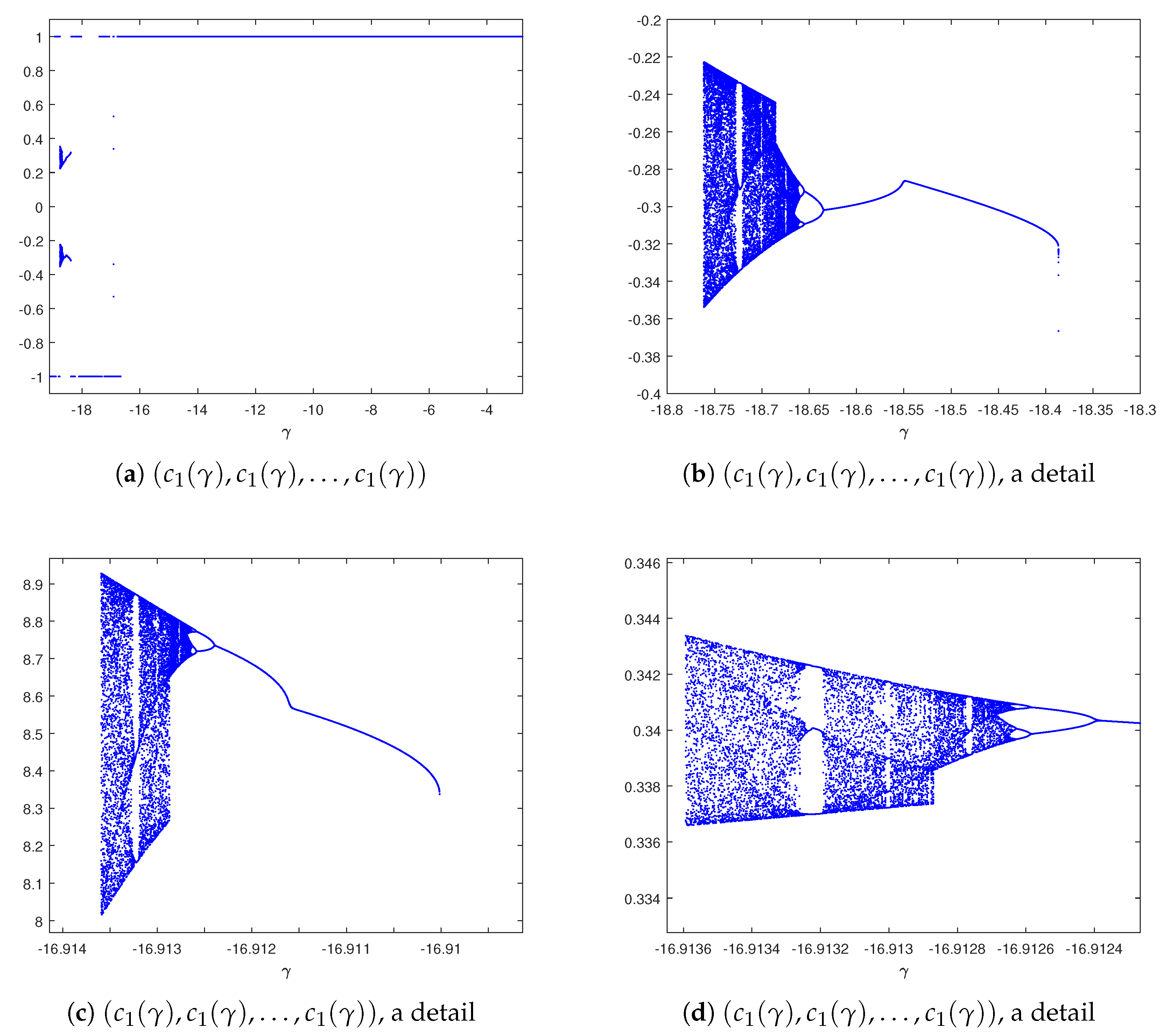
At this stage, bifurcation diagrams are employed to analyze the changes of performance for different ranges of $\gamma$. When $O{p}^4(z,\gamma )$ acts on a critical point, different performances are found after 500 iterations of the method, for each $\alpha$ divided in a mesh of 3000 points. It results in convergence to periodic orbits or to chaotic attractors.

In Figure 4 we see the bifurcation diagrams corresponding to the black region of the parameter line if $-{\displaystyle \frac{153}{8}}<\gamma <-{\displaystyle \frac{177}{64}}$ (Figure 3a). In Figure 4a, convergence to one root is seen, but also some period-doubling cascades appear in a small interval around $\gamma =-18.75$, including chaotic behavior (blue regions). There, strange attractors can be found.

To represent these strange attractors, we plot in the $(x_1,x_2)$-space the orbit of $z^{\left(0\right)}=(0.29,0.29)$ by $O{p}^4\left((x_1,x_2),\gamma \right)$, for several close values of $\gamma$ laying in the blue area of Figure 4b. For each $\gamma$, 2500 different starting guesses have been used and, their first 400 iterates are not plotted, the following 500 appear in blue color and the last ones are magenta. In Figure 5 it is observed as a parabolic strange fixed point, that bifurcates into periodic orbits of doubling periods, becomes chaotic while its orbits are dense in small regions of $(z_1,z_2)$-space.

This can be checked in the associated dynamical planes. Unstable performance is limited to values of $\gamma$ in the black regions of Figure 3. In Figure 6b an strange attractor is found for $\gamma =-18.75$, that was plotted in Figure 5b,c. Finally, in Figure 6c,d, the phase space for $\gamma =-18.45$ and $\gamma =-16.911$ respectively are represented. In them, 4-period orbits appear in yellow (the elements of the orbit are linked by yellow lines). In all cases, there exist more attracting orbits with symmetric coordinates.

We conclude that members of PM4$\left(\gamma \right)$ class are very stable. There not exist attractive strange fixed points and only in very narrow intervals of $\gamma$ there exists unstable performance.

4. Numerical Performance

We begin this section checking the applicability of our proposed methods PM4$\left(\gamma \right)$ by analyzing its behavior on some academic nonlinear systems. To get this aim, we select some members of the class with good qualitative properties and other with stability problems. This information is deduced from the results obtained in the previous section. Afterwards, we compare its behavior with that of other known methods on the same problems. The maximum number of iterates considered is 1000 and the stopping criterium is $\parallel z^{(i+1)}-z^{\left(i\right)}\parallel <{10}^{-150}$ or $\parallel F\left(z^{\left(i\right)}\right)\parallel <{10}^{-150}$. All the calculations have been made using Matlab R2019b with variable precision arithmetic with 1000 digits of mantissa, to minimize round-off errors.

We use in each example the Approximated Computational Order of Convergence, (ACOC), defined as

$$p\approx ACOC=\frac{ln\frac{\parallel z^{(i+1)}-z^{\left(i\right)}\parallel }{\parallel z^{\left(i\right)}-z^{(i-1)}\parallel }}{ln\frac{\parallel z^{\left(i\right)}-z^{(i-1)}\parallel }{\parallel z^{(i-1)}-z^{(i-2)}\parallel }},$$

and introduced in [23], that estimates numerically the theoretical order of convergence p.

We compare the proposed family, for different values of parameter $\gamma$, with class $M4\left(\beta \right)$ [12] for different values of $\beta$, with the extension of Jarratt’s scheme for nonlinear systems [24], whose iterative expression is

$$\begin{array}{ccc}\hfill y^{\left(i\right)}& =& z^{\left(i\right)}-\frac{2}{3}{\left[F^{\prime }\left(z^{\left(i\right)}\right)\right]}^{-1}F\left(z^{\left(i\right)}\right),\hfill \\ \hfill z^{(i+1)}& =& z^{\left(i\right)}-{[6F^{\prime }\left(y^{\left(i\right)}\right)-2F^{\prime }\left(z^{\left(i\right)}\right)]}^{-1}[3F^{\prime }\left(y^{\left(i\right)}\right)+F^{\prime }\left(z^{\left(i\right)}\right)]{\left[F^{\prime }\left(z^{\left(i\right)}\right)\right]}^{-1}F\left(z^{\left(i\right)}\right),i=0,1,2\dots \hfill \end{array}$$

and with the recent scheme $HM4$ of order four [1]

$$\begin{array}{ccc}\hfill y^{\left(i\right)}& =& z^{\left(i\right)}-{\left[F^{\prime }\left(z^{\left(i\right)}\right)\right]}^{-1}F\left(z^{\left(i\right)}\right),\hfill \\ \hfill z^{(i+1)}& =& z^{\left(i\right)}-H\left(z^{\left(i\right)}\right){\left[F^{\prime }\left(z^{\left(i\right)}\right)\right]}^{-1}F\left(z^{\left(i\right)}\right),i=0,1,2\dots ,\hfill \end{array}$$

with $H\left(z^{\left(i\right)}\right)=I+B_k^{-1}-B_k(2I-B_k)$, being $B_k={\left[F^{\prime }\left(z^{\left(i\right)}\right)\right]}^{-1}[z^{\left(i\right)},y^{\left(i\right)};F]$ and I the identity matrix.

In order to check the efficiency of the proposed methods, we compare the execution time (in seconds) only in Example 1, as in Example 2 there is no critical difference among the methods, in the third example there are many divergent results and in the fourth example, the execution time are qualitatively equal to those of Example 1.

Example 1.

The first nonlinear system is defined by

$$\left\{\begin{array}{c}{z}_1^2-z_2-19=0,\hfill \\ {z_2}^3/6-{z_1}^2+z_2-17=0.\hfill \end{array}\right.$$

In this example, we use the initial estimation $z^{\left(0\right)}={(1,2)}^T$.

In

Table 1. Numerical results for some $\gamma$ in PM4$\left(\gamma \right)$ in Example 1.

$\mathit{\gamma }$	$\overline{\mathit{z}}$	Iterations ( i)	$\parallel {\mathit{z}}^{\left(\mathit{i}\right)}-{\mathit{z}}^{(\mathit{i}-1)}\parallel$	$\parallel \mathit{F}\left({\mathit{z}}^{\left(\mathit{i}\right)}\right)\parallel$	ACOC	Cpu-Time
0	${(5,6)}^T$	6	8.2499 × 10${}^{-54}$	4.1678 × 10${}^{-214}$	3.9983	0.9038
10	${(5,6)}^T$	19	3.365 × 10${}^{-104}$	9.3749 × 10${}^{-415}$	4.0	2.7157
−10	${(-5,6)}^T$	53	1.5747 × 10${}^{-69}$	3.3897 × 10${}^{-276}$	4.0001	7.0803
−18.5	${(-5,6)}^T$	21	2.1718 × 10${}^{-72}$	4.1447 × 10${}^{-288}$	4.0	2.9821
−18.75	${(-5,6)}^T$	13	6.3187 × 10${}^{-48}$	1.773 × 10${}^{-189}$	4.0	1.8758
−16.9	${(-5,6)}^T$	11	5.9643 × 10${}^{-100}$	2.1312 × 10${}^{-398}$	4.0	1.5963

, we show the values of the last error estimations calculated, $\parallel z^{\left(i\right)}-z^{(i-1)}\parallel$ and $\parallel F\left(z^{\left(i\right)}\right)\parallel$, as well as the last value of the ACOC.

We observe in Table 1 that depending on the value of the parameter $\gamma$, method PM4$\left(\gamma \right)$ converges to $(5,6)$ or $(-5,6)$, meanwhile M4$\left(\beta \right)$ ( for $\beta =1/5$, $\beta =1$, and $\beta =5$), Jarratt’s and $HM4$ there is convergence only to $(5,6)$ (

Table 2. Numerical results by using known methods for Example 1.

Method	$\overline{\mathit{z}}$	Iterations (i)	$\parallel {\mathit{z}}^{\left(\mathit{i}\right)}-{\mathit{z}}^{(\mathit{i}-1)}\parallel$	$\parallel \mathit{F}\left({\mathit{z}}^{\left(\mathit{i}\right)}\right)\parallel$	ACOC	Cpu-Time
M4($\beta =\frac{1}{5}$)	${(5,6)}^T$	22	3.647 × 10${}^{-73}$	6.888 × 10${}^{-291}$	4.0	3.7779
M4($\beta =1$)	${(5,6)}^T$	27	1.368 × 10${}^{-61}$	1.136 × 10${}^{-244}$	4.0	4.6386
M4($\beta =5$)	${(5,6)}^T$	30	2.67 × 10${}^{-45}$	1.442 × 10${}^{-194}$	4.3227	5.2072
Jarratt	${(5,6)}^T$	6	2.4762 × 10${}^{-86}$	2.0268 × 10${}^{-344}$	3.9982	0.6515
HM4	${(5,6)}^T$	17	4.476 × 10${}^{-72}$	9.287 × 10${}^{-286}$	4.0	4.6644

). The values $\parallel z^{\left(i\right)}-z^{(i-1)}\parallel$ are in general better or similar of that of M4($\beta =1/5$), method of order 5.

Example 2.

$$\left\{\begin{array}{c}cos\left(z_2\right)-sin\left(z_1\right)=0,\hfill \\ z_1-1/z_2=0.\hfill \end{array}\right.$$

The numerical results for this test system are displayed in

Table 3. Numerical results with different $\gamma$ in PM4$\left(\gamma \right)$ for Example 2.

$\mathit{\gamma }$	Iterations (i)	$\parallel {\mathit{z}}^{\left(\mathit{i}\right)}-{\mathit{z}}^{(\mathit{i}-1)}\parallel$	$\parallel \mathit{F}\left({\mathit{z}}^{\left(\mathit{i}\right)}\right)\parallel$	ACOC
0	5	6.2248 × 10${}^{-105}$	2.7218 × 10${}^{-419}$	4.0
10	5	4.2537 × 10${}^{-66}$	8.966 × 10${}^{-264}$	4.0
−10	5	3.4263 × 10${}^{-121}$	1.1685 × 10${}^{-484}$	4.0006
−18.5	5	3.6569 × 10${}^{-98}$	3.4494 × 10${}^{-393}$	4.0035
−18.75	5	8.4703 × 10${}^{-98}$	8.8311 × 10${}^{-392}$	4.011
−16.9	5	5.9213 × 10${}^{-101}$	3.7153 × 10${}^{-404}$	4.0272

and

Table 4. Numerical results by using known methods for Example 2.

Method	Iterations (i)	$\parallel {\mathit{z}}^{\left(\mathit{i}\right)}-{\mathit{z}}^{(\mathit{i}-1)}\parallel$	$\parallel \mathit{F}\left({\mathit{z}}^{\left(\mathit{i}\right)}\right)\parallel$	ACOC
M4 ($\beta =\frac{1}{5}$)	5	2.085 × 10${}^{-145}$	1.048 × 10${}^{-581}$	4.0
M4 ($\beta =1$)	5	5.123 × 10${}^{-139}$	3.184 × 10${}^{-556}$	4.0
M4 ($\beta =5$)	5	1.541 × 10${}^{-131}$	2.011 × 10${}^{-526}$	3.9536
Jarratt	5	2.2611 × 10${}^{-107}$	4.6011 × 10${}^{-429}$	4.0
HM4	5	1.973 × 10${}^{-86}$	3.34 × 10${}^{-345}$	4.0

, where we show the same information than in the previous example. The initial estimation used is $z^{\left(0\right)}={(1,4)}^T$, being the solution obtained $\overline{z}\approx {(0.203,4.915)}^T$ in all the cases shown.

We observe in Table 3 and Table 4 that the PM4$\left(\gamma \right)$ get on a better ACOC that M4 ($\beta =5$) with the same number of iterations, being the results similar to those of M4 ($\beta =1/5$, $\beta =1$), Jarratt’s scheme and $HM4$.

Example 3.

The third example is given by the system:

$$z_i-1.5sin\left(\sum _{j=1,j\ne i}^{20}{z}_j\right)=0,i=1,\dots ,20.$$

We show the numerical results of the initial estimation $z^{\left(0\right)}={(1.25,\dots ,1.25)}^T$ in

Table 5. Numerical results for some $\gamma$ in PM4$\left(\gamma \right)$ for Example 3.

$\mathit{\gamma }$	$\overline{\mathit{z}}$	Iterations (i)	$\parallel {\mathit{z}}^{\left(\mathit{i}\right)}-{\mathit{z}}^{(\mathit{i}-1)}\parallel$	$\parallel \mathit{F}\left({\mathit{z}}^{\left(\mathit{i}\right)}\right)\parallel$	ACOC
0	${(1.032,\cdots ,1.032)}^T$	8	1.7477 × 10${}^{-47}$	3.6777 × 10${}^{-185}$	3.9997
10	${(1.134,\cdots ,1.134)}^T$	10	1.0923 × 10${}^{-64}$	3.1607 × 10${}^{-253}$	4.0
−10	-	diverge	-	-
−18.5	-	diverge	-	-
−18.75	-	diverge	-	-
−16.9	-	diverge	-	-

and

Table 6. Numerical results by using known methods for Example 3.

Method	$\overline{\mathit{z}}$	Iterations (i)	$\parallel {\mathit{z}}^{\left(\mathit{i}\right)}-{\mathit{z}}^{(\mathit{i}-1)}\parallel$	$\parallel \mathit{F}\left({\mathit{z}}^{\left(\mathit{i}\right)}\right)\parallel$	ACOC
M4 ($\beta =\frac{1}{5}$)	${(0.6864,\cdots ,0.6864)}^T$	5	2.28 × 10${}^{-63}$	4.655 × 10${}^{-249}$	4.0
M4 ($\beta =1$)	${(0.4789,\cdots ,0.4789)}^T$	46	1.323 × 10${}^{-88}$	1.128 × 10${}^{-350}$	4.0
M4 ($\beta =5$)	-	diverge	-	-	-
Jarratt	${(1.4224,\cdots ,1.4224)}^T$	6	1.9644 × 10${}^{-52}$	3.01 × 10${}^{-204}$	3.9999
HM4	${(-1.1134,\cdots ,-1.1134)}^T$	5	8.326 × 10${}^{-54}$	4.93 × 10${}^{-210}$	3.9999

. We note that in this case there are different behaviors depending on the value of $\gamma$. This is consistent with the results predicted in the dynamical study. It should be noticed that the method also diverges for M4 ($\beta =5$). In general, the method with best performance for this example is $HM4$.

We also observe that the stability of the method depends on the initial condition, for example, in the case of using the initial condition $z^{\left(0\right)}={(1,\dots ,1)}^T$ all the analyzed methods converge to $z^{\left(0\right)}={(1.032,\dots ,1.032)}^T$ with acceptable errors and a low number of iterations (4 or 5 in general), showing also an adequate ACOC. However, if we consider as initial condition the point $z^{\left(0\right)}={(0.25,\dots ,0.25)}^T$ all methods diverge.

Example 4.

The fourth example is:

$$\begin{array}{ccc}{z}_i{z}_{i+1}-1\hfill & =& 0,i=1,\dots ,98,\hfill \\ z_1{z}_{99}-1\hfill & =& 0.\hfill \end{array}$$

In this case we consider two initial estimations. The numerical results for $z^{\left(0\right)}={(0.1,\dots ,0.1)}^T$ are displayed in

Table 7. Numerical results with different $\gamma$ in PM4$\left(\gamma \right)$ for Example 4.

$\mathit{\gamma }$	$\overline{\mathit{z}}$	Iteracions (i)	$\parallel {\mathit{z}}^{\left(\mathit{i}\right)}-{\mathit{z}}^{(\mathit{i}-1)}\parallel$	$\parallel \mathit{F}\left({\mathit{z}}^{\left(\mathit{i}\right)}\right)\parallel$	ACOC
0	${(1,\dots ,1)}^T$	6	2.3769 × 10${}^{-64}$	1.1701 × 10${}^{-258}$	4.0
10	${(1,\dots ,1)}^T$	12	2.7217 × 10${}^{-48}$	1.3016 × 10${}^{-193}$	3.9999
−10	${(-1,\dots ,-1)}^T$	8	1.5339 × 10${}^{-45}$	9.0707 × 10${}^{-183}$	4.0003
−18.5	${(-1,\dots ,-1)}^T$	12	7.3866 × 10${}^{-137}$	9.953 × 10${}^{-548}$	4.0
−18.75	-	diverge	-	-	-
−16.9	${(-1,\dots ,-1)}^T$	7	3.2074 × 10${}^{-61}$	3.1986 × 10${}^{-245}$	4.0

and

Table 8. Numerical results by using known methods for Example 4.

Method	$\overline{\mathit{z}}$	Iterations (i)	$\parallel {\mathit{z}}^{\left(\mathit{i}\right)}-{\mathit{z}}^{(\mathit{i}-1)}\parallel$	$\parallel \mathit{F}\left({\mathit{z}}^{\left(\mathit{i}\right)}\right)\parallel$	ACOC
M4 ($\beta =\frac{1}{5}$)	${(-1,\dots ,-1)}^T$	13	8.741 × 10${}^{-58}$	7.112 × 10${}^{-232}$	4.0
M4 ($\beta =1$)	${(-1,\dots ,-1)}^T$	15	2.887 × 10${}^{-107}$	7.05 × 10${}^{-430}$	4.0
M4 ($\beta =5$)	${(-1,\dots ,-1)}^T$	15	3.404 × 10${}^{-96}$	8.165 × 10${}^{-482}$	5.0
Jarratt	${(1,\dots ,1)}^T$	6	1.1404 × 10${}^{-88}$	4.293 × 10${}^{-356}$	4.0
HM4	${(1,\dots ,1)}^T$	12	3.4 × 10${}^{-69}$	4.95 × 10${}^{-276}$	4.0

. The method converges to both different solutions, ${(1,\dots ,1)}^T$ and ${(-1,\dots ,-1)}^T$, depending on the value of the parameter.

As we can observe in Table 8 we get similar o better values for $\parallel z^{\left(i\right)}-z^{(i-1)}\parallel$ and $\parallel F\left(z^i\right)\parallel$ getting an ACOC equal to 4 or very close to 4.

For the initial estimation $z^{\left(0\right)}={(-20,\dots ,-20)}^T$, a very far value from the solution, the numerical results are displayed in

Table 9. Numerical results with different $\gamma$ in PM4$\left(\gamma \right)$ for Example 4.

$\mathit{\gamma }$	$\overline{\mathit{z}}$	Iterations (i)	$\parallel {\mathit{z}}^{\left(\mathit{i}\right)}-{\mathit{z}}^{(\mathit{i}-1)}\parallel$	$\parallel \mathit{F}\left({\mathit{z}}^{\left(\mathit{i}\right)}\right)\parallel$	ACOC
0	${(-1,\dots ,-1)}^T$	7	8.946 × 10${}^{-147}$	2.348 × 10${}^{-588}$	4.0
10	${(-1,\dots ,-1)}^T$	8	4.1718 × 10${}^{-110}$	7.1844 × 10${}^{-441}$	4.0
−10	${(-1,\dots ,-1)}^T$	6	3.0908 × 10${}^{-74}$	1.4956 × 10${}^{-297}$	4.0
−18.5	-	diverge	-	-	-
−18.75	-	diverge	-	-	-
−16.9	${(-1,\dots ,-1)}^T$	6	3.7482 × 10${}^{-100}$	5.9656 × 10${}^{-401}$	4.0

and

Table 10. Numerical results by using known methods for Example 4.

Method	$\overline{\mathit{z}}$	Iterations (i)	$\parallel {\mathit{z}}^{\mathit{i}}-{\mathit{z}}^{\mathit{i}-1}\parallel$	$\parallel \mathit{F}\left({\mathit{z}}^{\mathit{i}}\right)\parallel$	ACOC
M4 ($\beta =\frac{1}{5}$)	${(-1,\cdots ,-1)}^T$	7	2.347 × 10${}^{-80}$	3.694 × 10${}^{-322}$	4.0
M4 ($\beta =1$)	${(-1,\cdots ,-1)}^T$	7	8.187 × 10${}^{-88}$	4.56 × 10${}^{-352}$	4.0
M4 ($\beta =5$)	${(-1,\cdots ,-1)}^T$	6	1.447 × 10${}^{-48}$	1.133 × 10${}^{-243}$	5.0
Jarratt	${(1,\cdots ,1)}^T$	6	6.165 × 10${}^{-44}$	3.6677 × 10${}^{-177}$	3.9997
HM4	${(-1,\cdots ,-1)}^T$	7	1.03× 10${}^{-90}$	4.165× 10${}^{-362}$	4.0

where we can see that for the convergent values of the dynamical plane, the method is stable, showing similar or better behavior to that of Jarratt and M4$\left(\beta \right)$ for $\beta =1/5$, $\beta =1$ and $\beta =5$ (see $\parallel z^{\left(i\right)}-z^{(i-1)}\parallel$ ) and $\parallel F\left(z^i\right)\parallel$, with 4 for the ACOC value.

5. Conclusions

A parametric family of two-steps iterative methods for solving nonlinear systems has been designed. This class contains other known schemes, for particular values of the parameter, and has fourth order of convergence for any value of the parameter. We have studied the stability of this family on quadratic polynomial systems, in terms of the values of the parameter. This analysis allows us to detect the most stable elements of the class and those with chaotical behavior. Some numerical test confirm the dynamical and theoretical results.

References

1. Cordero, A.; García-Villalba, E.; Torregrosa, J.R.; Triguero, P. Convergence and stability of a parametric class of iterative schemes for solving nonlinear systems. Mathematics 2021, 9, 86. [Google Scholar] [CrossRef]
2. Amiri, A.; Cordero, A.; Darvishi, M.T.; Torregrosa, J.R. A fast algorithm to solve systems of nonlinear equations. Comput. Appl. Math. 2019, 354, 242–258. [Google Scholar] [CrossRef]
3. Chicharro, F.I.; Cordero, A.; Garrido, N.; Torregrosa, J.R. A new efficient parametric family of iterative methods for solving nonlinear systems. Differ. Equ. Appl. 2019, 25, 1454–1467. [Google Scholar] [CrossRef]
4. Singh, A. An efficient fifth-order Steffensen-type method for solving systems of nonlinear equations. Int. J. Comput. Sci. Math. 2018, 9, 501–514. [Google Scholar] [CrossRef]
5. Sharma, J.R.; Arora, H. Efficient derivative-free numerical methods for solving systems of nonlinear equations. Comput. Appl. Math. 2016, 35, 269–284. [Google Scholar] [CrossRef]
6. Wang, X.; Zhang, T.; Qian, W.; Teng, M. Seventh-order derivative-free iterative method for solving nonlinear systems. Numer. Algorithms 2015, 70, 545–558. [Google Scholar] [CrossRef]
7. Artidiello, S.; Cordero, A.; Torregrosa, J.R.; Vassileva, M.P. Multidimensional generalization of iterative methods for solving nonlinear problems by means of weight-function procedure. Appl. Math. Comput. 2015, 268, 1064–1071. [Google Scholar] [CrossRef] [Green Version]
8. Sharma, J.R.; Guha, R.K.; Sharma, R. An efficient fourth-order weighted-Newton method for systems of nonlinear equations. Numer. Algorithms 2013, 62, 307–323. [Google Scholar] [CrossRef]
9. Cordero, A.; Maimó, J.G.; Torregrosa, J.R.; Vassileva, M.P. Iterative Methods with Memory for Solving Systems of Nonlinear Equations Using a Second Order Approximation. Mathematics 2019, 7, 1069. [Google Scholar] [CrossRef] [Green Version]
10. Chicharro, F.I.; Cordero, A.; Garrido, N.; Torregrosa, J.R. On the improvement of the order of convergence of iterative methods for solving nonlinear systems by means of memory. Appl. Math. Lett. 2020, 104, 106277. [Google Scholar] [CrossRef]
11. Wang, X.; Jin, Y.; Zhao, Y. Derivative-free iterative methods with some Kurchatov-type accelerating parameters for solving nonlinear sistems. Symmetry 2021, 13, 943. [Google Scholar] [CrossRef]
12. Cordero, A.; Gutiérrez, J.M.; Magreñan, A.A.; Torregrosa, J.R. Stability analysis of a parametric family of iterative methods for solving nonlinear models. Appl. Math Comput. 2016, 285, 26–40. [Google Scholar] [CrossRef]
13. Arroyo, V.; Cordero, A.; Torregrosa, J.R. Approximation of artificial satellites’ preliminary orbits: The efficiency challeng. Math. Comput. Model. 2011, 54, 1802–1807. [Google Scholar] [CrossRef]
14. Cordero, A.; Hueso, J.L.; Martínez, E.; Torregrosa, J.R. A modified Newton-Jarratt’s composition. Numer. Algorithms 2010, 55, 87–99. [Google Scholar] [CrossRef]
15. Sharma, J.R.; Arora, H. Efficient Jarratt-like methods for solving systems of nonlinear equations. Calcolo 2014, 51, 193–210. [Google Scholar] [CrossRef]
16. Cordero, A.; Soleymani, F.; Torregrosa, J.R. Dynamical analysis of iterative methods for nonlinear systems or how to deal with the dimension? Appl. Math. Comput. 2014, 244, 398–412. [Google Scholar] [CrossRef]
17. Hueso, J.L.; Martínez, E.; Teruel, C. Convergence, effiency and dinamimics of new fourth and sixth order families of iterative methods for nonlinear systems. Comput. Appl. Math. 2015, 275, 412–420. [Google Scholar] [CrossRef]
18. Behl, R.; Sarría, I.; González, R.; Magreñán, A.A. Highly efficient family of iterative methods for solving nonlinear models. Comput. Appl. Math. 2019, 346, 110–132. [Google Scholar] [CrossRef]
19. Amiri, A.; Cordero, A.; Darvishi, M.T.; Torregrosa, J.R. Stability analysis of Jacobian-free Newton’s iterative method. Algorithms 2019, 12, 236. [Google Scholar] [CrossRef] [Green Version]
20. Robinson, R.C. An Introduction to Dynamical Systems, Continous and Discrete; Americal Mathematical Society: Providence, RI, USA, 2012. [Google Scholar]
21. Devaney, R.L. An Introduction to Chaotic Dynamical Systems, Advances in Mathematics and Engineering; CRC Press: Boca Raton, FL, USA, 2003. [Google Scholar]
22. Chicharro, F.I.; Cordero, A.; Torregrosa, J.R. Drawing dynamical and parameters planes of iterative families and methods. Sci. World J. 2013, 2013, 780153. [Google Scholar] [CrossRef] [PubMed]
23. Cordero, A.; Torregrosa, J.R. Variants of Newton’s method using fifth-order quadrature formulas. Appl. Math. Comput. 2007, 190, 686–698. [Google Scholar] [CrossRef]
24. Jarratt, P. Some fourth order multipoint iterative methods for solving equations. Math. Comput. 1966, 20, 434–437. [Google Scholar] [CrossRef]
Figure 1. Stability of the fixed points through their related eigenvalues.
Fractalfract 05 00125 g001
Figure 2. Stable dynamical planes of O p ( z , γ ) .
Fractalfract 05 00125 g002
Figure 3. Parameter lines of O p 4 ( z , γ ) .
Fractalfract 05 00125 g003
Figure 4. Feigenbaum diagrams of O p 4 ( z , γ ) for 153 8 < γ < 177 64 .
Fractalfract 05 00125 g004
Figure 5. Strange attractors of O p 4 ( z , γ ) for γ in a blue doubling-period cascade.
Fractalfract 05 00125 g005
Figure 6. Unstable dynamical planes of O p 4 ( z , γ ) on p ( z ) .
Fractalfract 05 00125 g006