Qualitative Study on Solutions of a Hadamard Variable Order Boundary Problem via the Ulam–Hyers–Rassias Stability

Abstract

In this paper, the existence, uniqueness and stability of solutions to a boundary value problem of nonlinear FDEs of variable order are established. To do this, we first investigate some aspects of variable order operators of Hadamard type. Then, with the help of the generalized intervals and piecewise constant functions, we convert the variable order Hadamard FBVP to an equivalent standard Hadamard BVP of the fractional constant order. Further, two fixed point theorems due to Schauder and Banach are used and, finally, the Ulam–Hyers–Rassias stability of the given variable order Hadamard FBVP is examined. These results are supported with the aid of a comprehensive example.

1. Introduction

The primitive idea of fractional calculus is to constitute the rational numbers in the order of derivation operators with natural numbers. Although this idea seems elementary and simple, it involves remarkable effects and outcomes which describe many physical and natural phenomena accurately. For this reason, research into both of the theoretical and practical aspects of boundary value problems has attracted the focus of many mathematicians in international academic institutions [1,2,3,4,5,6,7,8,9,10,11,12,13,14,15,16,17,18,19,20]. A main difference and novelty in this investigation is the application of the concept of variable order operators. These versions of variable order operators, which are dependent on their power-law kernel, can explain and model several hereditary aspects of various phenomena [21,22,23]. Generally, it is usually difficult to solve variable order FBVPs and obtain their analytical solution; hence, some numerical methods are introduced for the approximation of solutions to different FBVPs of variable order. In relation to the study of the existence theory to FBVPs of variable order, we point out some of them. In [24], Zhang studied solutions of a 2-point FBVP of variable order involving singular FDEs. Some years later, Zhang and Hu [25] presented the existence results for approximate solutions of a variable order fractional IVP on the half-axis. Recently, Refice et al. [26] investigated the Hadamard FBVP of variable order by means of the Kuratowski MNC method. In 2021, Bouazza et al. [27] considered a variable order multiterm BVP and derived their results by means of fixed point methods. For other instances, refer to [28,29,30,31].

In [32], Benchohra et al. studied the existence and Ulam-stability for the following implicit FBVP for the constant order $\mathrm{w}$ given by

$$\left\{\begin{array}{c}{}^H{D}_{1^{+}}^{\mathrm{w}}\mathrm{x}\left(t\right)=\psi (t,\mathrm{x}\left(t\right),{}^H{D}_{1^{+}}^{\mathrm{w}}),t\in \mathbb{I}:=[1,T],T>1,0<\mathrm{w}\le 1\hfill \\ \mathrm{x}\left(1\right)={\mathrm{x}}_1,\hfill \end{array}\right.$$

in which ${}^H{D}_{1^{+}}^{\mathrm{w}}$ is the ${\mathrm{w}}^{\mathrm{th}}$-constant order Hadamard operator and $\psi :\mathbb{I}\times {\mathbb{R}}^2\to \mathbb{R}$ is a function with some properties defined for it.

Motivated by the above mentioned articles and by the given Benchohra’s FBVP [32], in this manuscript, we deal with some qualitative aspects of solutions to the following FBVP of Hadamard variable order type with terminal conditions as

$$\left\{\begin{array}{c}\left({}^H{D}_{1^{+}}^{\mathrm{w}\left(t\right)}\mathrm{x}\right)\left(t\right)=\psi (t,\mathrm{x}\left(t\right)),t\in \mathbb{I}:=[1,T],\hfill \\ \mathrm{x}\left(1\right)=0,\mathrm{x}\left(T\right)=0,\hfill \end{array}\right.$$

(1)

in which $1<T<+\infty$, $\mathrm{w}\left(t\right):[1,T]\to (1,2]$, $\psi :\mathbb{I}\times \mathbb{R}\to \mathbb{R}$ is a continuous function and ${}^H{D}_{1^{+}}^{\mathrm{w}\left(t\right)}$ illustrates the Hadamard derivative of variable order $\mathrm{w}\left(t\right)$.

The purpose of our study is to propose new criteria on the uniqueness and existence for solutions of the Hadamard variable order FBVP (1). Additionally, we investigate the stability criterion of the obtained solution of the Hadamard variable order FBVP (1) in the sense of Ulam–Hyers–Rassias.

Ultimately, the remaining part of our research manuscript is arranged as follows. In Section 2, some preliminaries and properties of the variable order operators are introduced. In Section 3, new existence conditions are obtained based on the standard functional analysis techniques. The Ulam–Hyers–Rassias stability behavior is investigated in the sequel of this section. An example is given in Section 4 to illustrate the application of our main results. In Section 5, we indicate conclusions.

2. Auxiliary Notions

This section is devoted to recall some notions and definitions and auxiliary propositions which are used later.

Definition 1.

[33,34] Let $1\le a<b<+\infty$ and $\mathrm{w}:[a,b]\to (0,+\infty )$. The Hadamard integral of variable order $\mathrm{w}\left(t\right)$ for ψ is defined by

$$\left({}^H{I}_{a^{+}}^{\mathrm{w}\left(t\right)}\psi \right)\left(t\right)=\frac{1}{\mathsf{\Gamma }\left(\mathrm{w}\right(t\left)\right)}{\int }_a^t{(log\frac{t}{s})}^{\mathrm{w}\left(t\right)-1}\frac{\psi \left(s\right)}{s}ds,t>a,$$

(2)

if the right-hand side integral exists.

Definition 2.

[33,34] Let $k\in \mathbb{N}$ and $\mathrm{w}:[a,b]\to (k-1,k)$. The Hadamard derivative of variable order $\mathrm{w}\left(t\right)$ for ψ is defined by

$$\left({}^H{D}_{a^{+}}^{\mathrm{w}\left(t\right)}\psi \right)\left(t\right)=\frac{1}{\mathsf{\Gamma }(k-\mathrm{w}(t\left)\right)}{\left(t\frac{d}{dt}\right)}^k{\int }_a^t{(log\frac{t}{s})}^{k-\mathrm{w}\left(t\right)-1}\frac{\psi \left(s\right)}{s}ds,t>a,$$

(3)

if the right-hand side integral exists.

It is notable that if $\mathrm{w}\left(t\right)$ is assumed to be a constant function $\mathrm{w}$, then the Hadamard variable order fractional operators (2)–(3) are reduced to the usual Hadamard fractional operators; see [33,34,35]. Some applied properties of such variable order operators are as follows:

Proposition 1.

[35] For $a>1$, the general solution of the linear FDE

$${}^H{D}_{a^{+}}^{\mathrm{w}}\psi =0$$

has the following structure

$$\psi \left(t\right)=d_1{(log\frac{t}{a})}^{\mathrm{w}-1}+d_2{(log\frac{t}{a})}^{\mathrm{w}-2}+\cdots +d_k{(log\frac{t}{a})}^{\mathrm{w}-k}$$

for each $d_i\in \mathbb{R},$$i=1,2,\cdots ,k$. Here, $k-1<\mathrm{w}\le k$.

Proposition 2.

[35] Setting $a>1$, $\psi \in L(a,b)$, ${}^H{D}_{a^{+}}^{\mathrm{w}}\psi \in L(a,b)$, we have

$${}^H{I}_{a^{+}}^{\mathrm{w}}\left({}^H{D}_{a^{+}}^{\mathrm{w}}\psi \right)\left(t\right)=\psi \left(t\right)+d_1{(log\frac{t}{a})}^{\mathrm{w}-1}+d_2{(log\frac{t}{a})}^{\mathrm{w}-2}+\cdots +d_k{(log\frac{t}{a})}^{\mathrm{w}-k}$$

for $d_i\in \mathbb{R},$$i=1,2,\dots ,k$. Here, $k-1<\mathrm{w}\le k$.

Proposition 3.

[35] Let $\mathrm{w}>0$, $a>1$, $\psi \in L(a,b)$. Then, we have

$${}^H{D}_{a^{+}}^{\mathrm{w}}\left({}^H{I}_{a^{+}}^{\mathrm{w}}\psi \right)\left(t\right)=\psi \left(t\right).$$

Proposition 4.

[35] Let ${\mathrm{w}}_1,{\mathrm{w}}_2>0$, $a>1$, $\psi \in L(a,b)$. Then, we have

$${}^H{I}_{a^{+}}^{{\mathrm{w}}_1}\left({}^H{I}_{a^{+}}^{{\mathrm{w}}_2}\psi \right)\left(t\right)={}^H{I}_{a^{+}}^{{\mathrm{w}}_2}\left({}^H{I}_{a^{+}}^{{\mathrm{w}}_1}\psi \right)\left(t\right)={}^H{I}_{a^{+}}^{{\mathrm{w}}_1+{\mathrm{w}}_2}\psi \left(t\right).$$

Remark 1.

Note that for general functions ${\mathrm{w}}_1$ and ${\mathrm{w}}_2$, the semigroup property is not fulfilled, i.e.,

$${}^H{I}_{a^{+}}^{{\mathrm{w}}_1\left(t\right)}\left({}^H{I}_{a^{+}}^{{\mathrm{w}}_2\left(t\right)}\psi \right)\left(t\right)\ne {}^H{I}_{a^{+}}^{{\mathrm{w}}_1\left(t\right)+{\mathrm{w}}_2\left(t\right)}\psi \left(t\right),a>1.$$

To see this, we provide an example.

Example 1.

Let

$${\mathrm{w}}_1\left(t\right)=\left\{\begin{array}{c}t-1,t\in [1,2],\hfill \\ t-2,t\in (2,4],\hfill \end{array}\right.{\mathrm{w}}_2\left(t\right)=\left\{\begin{array}{c}1,t\in [1,2]\hfill \\ 2,t\in (2,4],\hfill \end{array}\right.\psi \left(t\right)=1,t\in [1,4].$$

Then

$$\begin{array}{ccc}\hfill {}^H{I}_{1^{+}}^{{\mathrm{w}}_1\left(t\right)}\left({}^H{I}_{1^{+}}^{{\mathrm{w}}_2\left(t\right)}\psi \right)\left(t\right)& =& \frac{1}{\mathsf{\Gamma }\left({\mathrm{w}}_1\left(t\right)\right)}{\int }_1^t\frac{1}{s}{(log\frac{t}{s})}^{{\mathrm{w}}_1\left(t\right)-1}\left[\frac{1}{\mathsf{\Gamma }\left({\mathrm{w}}_2\left(s\right)\right)}{\int }_1^s\frac{1}{\tau }{(log\frac{s}{\tau })}^{{\mathrm{w}}_2\left(s\right)-1}\psi \left(\tau \right)d\tau \right]ds\hfill \\ & =& \frac{1}{\mathsf{\Gamma }(t-1)}{\int }_1^2\frac{1}{s}{(log\frac{t}{s})}^{t-2}\left[\frac{1}{\mathsf{\Gamma }\left(1\right)}{\int }_1^2\frac{1}{\tau }{(log\frac{s}{\tau })}^{1-1}d\tau +\frac{1}{\mathsf{\Gamma }\left(2\right)}{\int }_2^s\frac{1}{\tau }{(log\frac{s}{\tau })}^{2-1}d\tau \right]ds\hfill \\ & +& \frac{1}{\mathsf{\Gamma }(t-2)}{\int }_2^t\frac{1}{s}{(log\frac{t}{s})}^{t-3}\left[\frac{1}{\mathsf{\Gamma }\left(1\right)}{\int }_1^2\frac{1}{\tau }{(log\frac{s}{\tau })}^{1-1}d\tau +\frac{1}{\mathsf{\Gamma }\left(2\right)}{\int }_2^s\frac{1}{\tau }{(log\frac{s}{\tau })}^{2-1}d\tau \right]ds\hfill \\ & =& \frac{1}{\mathsf{\Gamma }(t-1)}{\int }_1^2\frac{1}{s}{(log\frac{t}{s})}^{t-2}\left[log2+\frac{1}{2}{(log\frac{s}{2})}^2\right]ds\hfill \\ & +& \frac{1}{\mathsf{\Gamma }(t-2)}{\int }_2^t\frac{1}{s}{(log\frac{t}{s})}^{t-3}\left[log2+\frac{1}{2}{(log\frac{s}{2})}^2\right]ds,\hfill \end{array}$$

and

$$\begin{array}{ccc}\hfill {}^H{I}_{1^{+}}^{{\mathrm{w}}_1\left(t\right)+{\mathrm{w}}_2\left(t\right)}\psi \left(t\right)& =& \frac{1}{\mathsf{\Gamma }({\mathrm{w}}_1\left(t\right)+{\mathrm{w}}_2\left(t\right))}{\int }_1^t\frac{1}{s}{(log\frac{t}{s})}^{{\mathrm{w}}_1\left(t\right)+{\mathrm{w}}_2\left(t\right)-1}h\left(s\right)ds.\hfill \end{array}$$

Now, we see that

$$\begin{array}{ccc}\hfill {}^H{I}_{1^{+}}^{{\mathrm{w}}_1\left(t\right)}\left({}^H{I}_{1^{+}}^{{\mathrm{w}}_2\left(t\right)}\psi \right)\left(t\right){|}_{t=3}& =& \frac{1}{\mathsf{\Gamma }\left(2\right)}{\int }_1^2\frac{1}{s}{(log\frac{3}{s})}^1\left[log2+\frac{1}{2}{(log\frac{s}{2})}^2)\right]ds\hfill \\ & +& \frac{1}{\mathsf{\Gamma }\left(1\right)}{\int }_2^3\frac{1}{s}{(log\frac{3}{s})}^{3-3}\left[log2+\frac{1}{2}{(log\frac{s}{2})}^2\right]ds\hfill \\ & =& log2{\int }_1^2\frac{1}{s}(log\frac{3}{s})ds+\frac{1}{2}{\int }_1^2\frac{1}{s}(log\frac{3}{s}){(log\frac{s}{2})}^{2}ds\hfill \\ & +& log2{\int }_2^3\frac{1}{s}ds+\frac{1}{2}{\int }_2^3\frac{1}{s}{(log\frac{s}{2})}^{2}ds\hfill \\ & =& \frac{log2}{2}[{(log3)}^2-{(log\frac{3}{2})}^2]+\frac{1}{24}[{(log3)}^4-{(log\frac{3}{2})}^4]+\frac{1}{4}{(log3)}^2{(log2)}^2\hfill \\ & -& \frac{1}{6}(log2){(log3)}^3+log2[(log3)-(log2)]+\frac{1}{6}{(log\frac{3}{2})}^3\hfill \\ & \simeq & 0.9013,\hfill \end{array}$$

and

$$\begin{array}{ccc}\hfill {}^H{I}_{1^{+}}^{{\mathrm{w}}_1\left(t\right)+{\mathrm{w}}_2\left(t\right)}\psi \left(t\right){|}_{t=3}& =& \frac{1}{\mathsf{\Gamma }({\mathrm{w}}_1\left(t\right)+{\mathrm{w}}_2\left(t\right))}{\int }_1^t\frac{1}{s}{(log\frac{t}{s})}^{{\mathrm{w}}_1\left(t\right)+{\mathrm{w}}_2\left(t\right)-1}\psi \left(s\right)ds\hfill \\ & =& \frac{1}{\mathsf{\Gamma }\left(3\right)}{\int }_1^2\frac{1}{s}{(log\frac{3}{s})}^{2}ds+\frac{1}{\mathsf{\Gamma }\left(3\right)}{\int }_2^3\frac{1}{s}{(log\frac{3}{s})}^{2}ds\hfill \\ & =& \frac{1}{\mathsf{\Gamma }\left(4\right)}[{(log3)}^3-{(log\frac{3}{2})}^3]+\frac{1}{\mathsf{\Gamma }\left(4\right)}{(log\frac{3}{2})}^3\hfill \\ & \simeq & 0.2209.\hfill \end{array}$$

Therefore, we obtain

$${}^H{I}_{1^{+}}^{{\mathrm{w}}_1\left(t\right)}\left({}^H{I}_{1^{+}}^{{\mathrm{w}}_2\left(t\right)}\psi \right)\left(t\right){|}_{t=3}\ne {}^H{I}_{1^{+}}^{{\mathrm{w}}_1\left(t\right)+{\mathrm{w}}_2\left(t\right)}\psi \left(t\right){|}_{t=3}.$$

Proposition 5.

Let $\mathbb{I}:=[1,T]$, where $1<T<+\infty$ and let $\mathrm{w}\in C(\mathbb{I},(1,2\left]\right)$. Then, for each

$$\psi \in C_g(\mathbb{I},\mathbb{R})=\{\psi \left(t\right)\in C(\mathbb{I},\mathbb{R}),{(logt)}^g\psi \left(t\right)\in C(\mathbb{I},\mathbb{R})\},0\le g\le 1,$$

the Hadamard variable order integral ${}^H{I}_{1^{+}}^{\mathrm{w}\left(t\right)}\psi \left(t\right)$ exists for each point on $\mathbb{I}$.

Proof. 

In view of the continuity of $\mathsf{\Gamma }\left(\mathrm{w}\right(t\left)\right)$, we verify that $M_{\mathrm{w}}={max}_{t\in \mathbb{I}}\left|{\displaystyle \frac{1}{\mathsf{\Gamma }\left(\mathrm{w}\right(t\left)\right)}}\right|$ exists. Take ${\mathrm{w}}^{*}={max}_{t\in \mathbb{I}}\left|\left(\mathrm{w}\left(t\right)\right)\right|$. In this case, for $1\le s\le t\le T$, one may write

$${(log\frac{t}{s})}^{\mathrm{w}\left(t\right)-1}\le 1,\mathrm{if}1\le \frac{t}{s}\le e,$$

and

$${(log\frac{t}{s})}^{\mathrm{w}\left(t\right)-1}\le {(log\frac{t}{s})}^{{\mathrm{w}}^{*}-1},\mathrm{if}\frac{t}{s}>e.$$

In addition, for $1\le {\displaystyle \frac{t}{s}}<+\infty$, we know that

$${(log\frac{t}{s})}^{\mathrm{w}\left(t\right)-1}\le max\{1,{(log\frac{t}{s})}^{{\mathrm{w}}^{*}-1}\}=M^{*}.$$

Thus, for each $\psi \in C_g(\mathbb{I},X)$ and by the definition of (2), we deduce that

$$\begin{array}{ccc}\hfill \left|\left({}^H{I}_{1^{+}}^{u\left(t\right)}\psi \right)\left(t\right)\right|& =& \frac{1}{\mathsf{\Gamma }\left(\mathrm{w}\right(t\left)\right)}{\int }_1^t{(log\frac{t}{s})}^{\mathrm{w}\left(t\right)-1}\frac{\left|\psi \right(s\left)\right|}{s}ds\hfill \\ & \le & M_{\mathrm{w}}{\int }_1^t{(log\frac{t}{s})}^{\mathrm{w}\left(t\right)-1}{(logs)}^{-g}{(logs)}^g\frac{\left|\psi \right(s\left)\right|}{s}ds\hfill \\ & \le & M_{\mathrm{w}}{M}^{*}{\int }_1^t\frac{1}{s}{(logs)}^{-g}\underset{s\in \mathbb{I}}{max}{(logs)}^g\left|\psi \left(s\right)\right|ds\hfill \\ & \le & M_{\mathrm{w}}{M}^{*}\underset{s\in \mathbb{I}}{max}{(logs)}^g{\psi }^{☆}{\int }_1^t\frac{1}{s}{(logs)}^{-g}ds\hfill \\ & \le & M_{\mathrm{w}}{M}^{*}\underset{s\in \mathbb{I}}{max}{(logs)}^g{\psi }^{☆}\frac{{(logT)}^{1-g}}{1-g}<\infty ,\hfill \end{array}$$

where ${\psi }^{☆}={max}_{t\in \mathbb{I}}\left|\psi \left(t\right)\right|$. It yields that the variable order Hadamard integral ${}^H{I}_{1^{+}}^{\mathrm{w}\left(t\right)}\psi \left(t\right)$ exists for every point on $\mathbb{I}$. □

Proposition 6.

Let $\mathrm{w}\in C(\mathbb{I},(1,2\left]\right)$. Then,

$${}^H{I}_{1^{+}}^{\mathrm{w}\left(t\right)}\psi \left(t\right)\in C(\mathbb{I},\mathbb{R})$$

for every $\psi \in C(\mathbb{I},\mathbb{R})$.

Proof. 

For any $t,t_{*}\in \mathbb{I}$ subject to $t_{*}\le t$ and $\psi \in C(\mathbb{I},\mathbb{R})$, we obtain

$$\begin{array}{cc}\hfill |{}^H{I}_{1^{+}}^{\mathrm{w}\left(t\right)}& \psi \left(t\right)-{}^H{I}_{1^{+}}^{\mathrm{w}\left(t_{*}\right)}\psi \left(t_{*}\right)|=|{\int }_1^t\frac{1}{\mathsf{\Gamma }\left(\mathrm{w}\right(t\left)\right)}{(log\frac{t}{s})}^{\mathrm{w}\left(t\right)-1}\frac{\psi \left(s\right)}{s}ds\hfill \\ \hfill & -{\int }_1^{t_{*}}\frac{1}{\mathsf{\Gamma }\left(\mathrm{w}\left(t_{*}\right)\right)}{(log\frac{t_{*}}{s})}^{\mathrm{w}\left(t_{*}\right)-1}\frac{\psi \left(s\right)}{s}ds|\hfill \\ \hfill & =|{\int }_0^1\frac{1}{\mathsf{\Gamma }\left(\mathrm{w}\right(t\left)\right)}\frac{(t-1)}{r(t-1)+1}{(log\frac{t}{r(t-1)+1})}^{\mathrm{w}\left(t\right)-1}\psi \left(r\right(t-1)+1)dr\hfill \\ \hfill & -{\int }_0^1\frac{1}{\mathsf{\Gamma }\left(\mathrm{w}\left(t_{*}\right)\right)}\frac{(t_{*}-1)}{r(t_{*}-1)+1}{(log\frac{t_{*}}{r(t_{*}-1)+1})}^{\mathrm{w}\left(t_{*}\right)-1}\psi (r(t_{*}-1)+1)dr|\hfill \\ \hfill & =\left|{\int }_0^1\right[\frac{1}{\mathsf{\Gamma }\left(\mathrm{w}\right(t\left)\right)}\frac{(t-1)}{r(t-1)+1}{(log\frac{t}{r(t-1)+1})}^{\mathrm{w}\left(t\right)-1}\psi \left(r\right(t-1)+1)\hfill \\ \hfill & -\frac{1}{\mathsf{\Gamma }\left(\mathrm{w}\right(t\left)\right)}\frac{(t_{*}-1)}{r(t_{*}-1)+1}{(log\frac{t}{r(t-1)+1})}^{\mathrm{w}\left(t\right)-1}\psi \left(r\right(t-1)+1)]dr\hfill \\ \hfill & +{\int }_0^1[\frac{1}{\mathsf{\Gamma }\left(\mathrm{w}\right(t\left)\right)}\frac{(t_{*}-1)}{r(t_{*}-1)+1}{(log\frac{t}{r(t-1)+1})}^{\mathrm{w}\left(t\right)-1}\psi \left(r\right(t-1)+1)\hfill \\ \hfill & -\frac{1}{\mathsf{\Gamma }\left(\mathrm{w}\right(t\left)\right)}\frac{(t_{*}-1)}{r(t_{*}-1)+1}{(log\frac{t_{*}}{r(t_{*}-1)+1})}^{\mathrm{w}\left(t_{*}\right)-1}\psi \left(r\right(t-1)+1)]dr\hfill \\ \hfill & +{\int }_0^1[\frac{1}{\mathsf{\Gamma }\left(\mathrm{w}\right(t\left)\right)}\frac{(t_{*}-1)}{r(t_{*}-1)+1}{(log\frac{t_{*}}{r(t_{*}-1)+1})}^{\mathrm{w}\left(t_{*}\right)-1}\psi \left(r\right(t-1)+1)\hfill \\ \hfill & -\frac{1}{\mathsf{\Gamma }\left(\mathrm{w}\left(t_{*}\right)\right)}\frac{(t_{*}-1)}{r(t_{*}-1)+1}{(log\frac{t_{*}}{r(t_{*}-1)+1})}^{\mathrm{w}\left(t_{*}\right)-1}\psi \left(r\right(t-1)+1)]dr\hfill \\ \hfill & +{\int }_0^1[\frac{1}{\mathsf{\Gamma }\left(\mathrm{w}\left(t_{*}\right)\right)}\frac{(t_{*}-1)}{r(t_{*}-1)+1}{(log\frac{t_{*}}{r(t_{*}-1)+1})}^{\mathrm{w}\left(t_{*}\right)-1}\psi \left(r\right(t-1)+1)\hfill \\ \hfill & -\frac{1}{\mathsf{\Gamma }\left(\mathrm{w}\left(t_{*}\right)\right)}\frac{(t_{*}-1)}{r(t_{*}-1)+1}{(log\frac{t_{*}}{r(t_{*}-1)+1})}^{\mathrm{w}\left(t_{*}\right)-1}\psi (r(t_{*}-1)+1)\left]dr\right|\hfill \\ \hfill & \le {\psi }^{☆}{\int }_0^1\frac{1}{\mathsf{\Gamma }\left(\mathrm{w}\right(t\left)\right)}{(log\frac{t}{r(t-1)+1})}^{\mathrm{w}\left(t\right)-1}|\frac{(t-1)}{r(t-1)+1}-\frac{(t_{*}-1)}{r(t_{*}-1)+1}|dr\hfill \\ \hfill & +{\psi }^{☆}{\int }_0^1\frac{1}{\mathsf{\Gamma }\left(\mathrm{w}\right(t\left)\right)}\frac{(t_{*}-1)}{r(t_{*}-1)+1}|{(log\frac{t}{r(t-1)+1})}^{\mathrm{w}\left(t\right)-1}-{(log\frac{t_{*}}{r(t_{*}-1)+1})}^{\mathrm{w}\left(t\right)-1}|dr\hfill \\ \hfill & +{\psi }^{☆}{\int }_0^1\frac{(t_{*}-1)}{r(t_{*}-1)+1}{(log\frac{t_{*}}{r(t_{*}-1)+1})}^{\mathrm{w}\left(t_{*}\right)-1}|\frac{1}{\mathsf{\Gamma }\left(\mathrm{w}\right(t\left)\right)}-\frac{1}{\mathsf{\Gamma }\left(\mathrm{w}\left(t_{*}\right)\right)}|dr\hfill \\ \hfill & +{\int }_0^1\frac{1}{\mathsf{\Gamma }\left(\mathrm{w}\left(t_{*}\right)\right)}\frac{(t_{*}-1)}{r(t_{*}-1)+1}{(log\frac{t_{*}}{r(t_{*}-1)+1})}^{\mathrm{w}\left(t_{*}\right)-1}|\psi (r(t-1)+1)-\psi (r(t_{*}-1)+1)|dr,\hfill \end{array}$$

where ${\psi }^{\star }={max}_{t\in \mathbb{I}}\left|\psi \left(t\right)\right|$. In view of the continuity of functions

$$\frac{(t-1)}{r(t-1)+1},{(log\frac{t}{r(t-1)+1})}^{\mathrm{w}\left(t\right)-1},\frac{1}{\mathsf{\Gamma }\left(\mathrm{w}\right(t\left)\right)},\psi \left(t\right),$$

we obtain that the integral ${}^H{I}_{1^{+}}^{\mathrm{w}\left(t\right)}\psi \left(t\right)$ is continuous at point $t_{*}$ and so we find that

$${}^H{I}_{1^{+}}^{\mathrm{w}\left(t\right)}\psi \left(t\right)\in C(\mathbb{I},\mathbb{R})$$

for each $\psi \left(t\right)\in C(\mathbb{I},\mathbb{R})$ which completes the proof. □

Definition 3.

[36,37,38]

(1)

A set $J\subset \mathbb{R}$ is termed as a generalized interval whenever it is either a standard interval, a point, or ∅.

(2)

By assuming J as a generalized interval, a finite set $\mathbb{P}$ consisting of generalized intervals contained in J is named a partition of J provided that every $\mathrm{w}\in J$ lies in exactly one of the generalized intervals E in $\mathbb{P}$.

(3)

By virtue of above notations, the function $g:J\to \mathbb{R}$ is defined to be a piecewise constant w.r.t. $\mathbb{P}$ whenever $\forall E\in \mathbb{P}$, g admits constant values on E.

To establish required results on the existence criterion of solutions for the supposed Hadamard variable order BVP (1), we apply the next theorem due to Schauder [35].

Theorem 1.

[35] Consider X and A as a Banach space and a closed convex bounded subset of X, respectively, and $\varphi :A\to A$ is compact and continuous. Then, ϕ admits at least one fixed point in A.

3. Existence Criterion and Ulam–Hyers–Rassias Stability

By $C(\mathbb{I},\mathbb{R})$, we denote the class of all continuous maps via the norm

$$\parallel \mathrm{x}\parallel =sup\left\{\right|\mathrm{x}\left(t\right)|,t\in \mathbb{I}\}.$$

In this case, $\left(C\right(\mathbb{I},\mathbb{R}),\parallel ·\parallel )$ is a Banach space. We present some needed assumptions:

(HP1) 

For $n\in \mathbb{N}$, define

$$\mathbb{P}=\{{\mathbb{I}}_1:=[0,T_1],{\mathbb{I}}_2:=(T_1,T_2],{\mathbb{I}}_3:=(T_2,T_3],\cdots ,{\mathbb{I}}_n:=(T_{n-1},T]\}$$

as a partition of the interval $\mathbb{I}$, and assume that $\mathrm{w}:\mathbb{I}\to (1,2]$ is a piecewise constant function w.r.t. $\mathbb{P}$; in other words

$$\mathrm{w}\left(t\right)=\sum _{i=1}^n{\mathrm{w}}_i{\mathcal{I}}_i\left(t\right)=\left\{\begin{array}{c}{\mathrm{w}}_1,\mathrm{if}t\in {\mathbb{I}}_1,\hfill \\ {\mathrm{w}}_2,\mathrm{if}t\in {\mathbb{I}}_2,\hfill \\ ⋮⋮⋮\hfill \\ {\mathrm{w}}_n,\mathrm{if}t\in {\mathbb{I}}_n,\hfill \end{array}\right.$$

in which $1<{\mathrm{w}}_i\le 2$ belong to $\mathbb{R}$, and ${\mathcal{I}}_i$ illustrates the indicator of ${\mathbb{I}}_i:=(T_{i-1},T_i],i\in {\mathbb{N}}_1^n$, (by assuming $T_0=1,T_n=T$) so that

$${\mathcal{I}}_i\left(t\right)=\left\{\begin{array}{c}1,\mathrm{for}t\in {\mathbb{I}}_i,\hfill \\ 0,\mathrm{for}\mathrm{o}.\mathrm{w}.\hfill \end{array}\right.$$

(HP2) 

For $0\le g\le 1$, let ${(logt)}^g\psi \in C(\mathbb{I}\times \mathbb{R},\mathbb{R})$ and $\exists \ell >0$ so that, ${(logt)}^g|\psi (t,{\mathrm{x}}_1)-\psi (t,{\mathrm{x}}_2)|\le \ell |{\mathrm{x}}_1-{\mathrm{x}}_2|,$ for any ${\mathrm{x}}_1,{\mathrm{x}}_2,\in \mathbb{R}$ and $t\in \mathbb{I}$.

In addition, by $E_i=C({\mathbb{I}}_i,\mathbb{R}),$ we denote the class of functions which form a Banach space via

$${\parallel \mathrm{x}\parallel }_{E_i}=\underset{t\in {\mathbb{I}}_i}{sup}\left|\mathrm{x}\left(t\right)\right|,$$

where $i\in \{1,2,\dots ,n\}$.

To prove the main results, we continue our analysis on the variable order Hadamard fractional boundary value problem (1) as follows.

By Equation (3), the differential equation of the variable order Hadamard FBVP (1) can be rewritten as

$$\frac{1}{\mathsf{\Gamma }(2-\mathrm{w}(t\left)\right)}{\left(t\frac{d}{dt}\right)}^2{\int }_1^t{(log\frac{t}{s})}^{1-\mathrm{w}\left(t\right)}\frac{\mathrm{x}\left(s\right)}{s}ds=\psi (t,\mathrm{x}\left(t\right)),t\in \mathbb{I}.$$

(4)

According to $\left(HP1\right)$, Equation (4) in every interval ${\mathbb{I}}_i$ can be represented by

$${\left(t\frac{d}{dt}\right)}^2\left(\frac{1}{\mathsf{\Gamma }(2-{\mathrm{w}}_1)}{\int }_1^{T_1}{(log\frac{t}{s})}^{1-{\mathrm{w}}_1}\frac{\mathrm{x}\left(s\right)}{s}ds+\cdots +\frac{1}{\mathsf{\Gamma }(2-{\mathrm{w}}_i)}{\int }_{T_{i-1}}^t{(log\frac{t}{s})}^{1-{\mathrm{w}}_i}\frac{\mathrm{x}\left(s\right)}{s}ds\right)=\psi (t,\mathrm{x}\left(t\right)),$$

(5)

for $t\in {\mathbb{I}}_i$. Now, we can state the definition of the solution to the variable order Hadamard FBVP (1) which is fundamental in the paper.

Definition 4.

We say that the variable order Hadamard FBVP (1) admits a solution, if the functions ${\mathrm{x}}_i,i=1,2,\dots ,n,$ exist such that ${\mathrm{x}}_i\in C([1,T_i],\mathbb{R})$ satisfies Equation (5) and ${\mathrm{x}}_i\left(1\right)=0={\mathrm{x}}_i\left(T_i\right)$.

In accordance with above contents, the differential equation of the variable order Hadamard FBVP (1) can be formulated as Equation (4), and accordingly can be written in the intervals ${\mathbb{I}}_i,i\in \{1,2,\dots ,n\}$ as Equation (5). So, for $0\le t\le T_{i-1}$, we assume $\mathrm{x}\left(t\right)\equiv 0$. In this case, Equation (5) is reduced to the following equation

$$\left({}^H{D}_{T_{i-1}^{+}}^{{\mathrm{w}}_i}\mathrm{x}\right)\left(t\right)=\psi (t,\mathrm{x}\left(t\right)),t\in {\mathbb{I}}_i.$$

From now on, we follow our study on the equivalent standard Hadamard FBVP which takes the form

$$\left\{\begin{array}{c}\left({}^H{D}_{T_{i-1}^{+}}^{{\mathrm{w}}_i}\mathrm{x}\right)\left(t\right)=\psi (t,\mathrm{x}\left(t\right)),t\in {\mathbb{I}}_i\hfill \\ \mathrm{x}\left(T_{i-1}\right)=0,\mathrm{x}\left(T_i\right)=0.\hfill \end{array}\right.$$

(6)

The next auxiliary proposition helps us to derive the existence criterion of solutions to the equivalent standard Hadamard FBVP (6).

Proposition 7.

The function $\mathrm{x}\in E_i$ is a solution of the equivalent standard Hadamard FBVP (6) if $\mathrm{x}$ satisfies

$$\mathrm{x}\left(t\right)=-{(log\frac{T_i}{T_{i-1}})}^{1-{\mathrm{w}}_i}{(log\frac{t}{T_{i-1}})}^{{\mathrm{w}}_i-1}{}^H{I}_{T_{i-1}^{+}}^{{\mathrm{w}}_i}\psi (T_i,\mathrm{x}\left(T_i\right))+{}^H{I}_{T_{i-1}^{+}}^{{\mathrm{w}}_i}\psi (t,\mathrm{x}\left(t\right)).$$

(7)

Proof. 

Let $\mathrm{x}\in E_i$ be the solution of the equivalent standard Hadamard FBVP (6). Now, applying the operator ${}^H{I}_{T_{i-1}^{+}}^{{\mathrm{w}}_i}$ to both sides of Equation (6) and by Proposition 2, we have

$$\begin{array}{c}\hfill \mathrm{x}\left(t\right)=d_1{(log\frac{t}{T_{i-1}})}^{{\mathrm{w}}_i-1}+d_2{(log\frac{t}{T_{i-1}})}^{{\mathrm{w}}_i-2}+{}^H{I}_{T_{i-1}^{+}}^{{\mathrm{w}}_i}\psi (t,\mathrm{x}\left(t\right)),t\in {\mathbb{I}}_i.\end{array}$$

By $\mathrm{x}\left(T_{i-1}\right)=0$ and the given hypothesis on the function $\psi$, it is obtained $d_2=0$. By considering $\mathrm{x}\left(t\right)$ satisfying $\mathrm{x}\left(T_i\right)=0$, we can obtain

$$d_1=-{(log\frac{T_i}{T_{i-1}})}^{1-{\mathrm{w}}_i}{}^H{I}_{T_{i-1}^{+}}^{{\mathrm{w}}_i}\psi (T_i,\mathrm{x}\left(T_i\right)).$$

Then,

$$\mathrm{x}\left(t\right)=-{(log\frac{T_i}{T_{i-1}})}^{1-{\mathrm{w}}_i}{(log\frac{t}{T_{i-1}})}^{{\mathrm{w}}_i-1}{}^H{I}_{T_{i-1}^{+}}^{{\mathrm{w}}_i}\psi (T_i,\mathrm{x}\left(T_i\right))+{}^H{I}_{T_{i-1}^{+}}^{{\mathrm{w}}_i}\psi (t,\mathrm{x}\left(t\right)),t\in {\mathbb{I}}_i.$$

Reversely, let $\mathrm{x}\in E_i$ be the solution of Equation (7). Then, by the continuity of ${(logt)}^g\psi$ and Proposition 3, one can simply follow that $\mathrm{x}$ is the solution of the equivalent standard Hadamard FBVP (6). □

The next result is based on Theorem 1.

Theorem 2.

Consider (HP1) and (HP2) and let $\psi :{\mathbb{I}}_i\times \mathbb{R}\to \mathbb{R}$ be a continuous function and

$$\frac{\ell \left({(log{T}_i)}^{1-g}-{(log{T}_{i-1})}^{1-g}\right)}{(1-g)\mathsf{\Gamma }\left({\mathrm{w}}_i\right)}{(log\frac{T_i}{T_{i-1}})}^{{\mathrm{w}}_i-1}<\frac{1}{2}.$$

Then, the variable order Hadamard FBVP (6) possesses a solution on $\mathbb{I}$.

Proof. 

We firstly convert the equivalent standard Hadamard FBVP (6) to a fixed-point problem. Define

$$W:E_i\to E_i,i\in {\mathbb{N}}_1^n,$$

by

$$\begin{array}{cc}\hfill W\mathrm{x}\left(t\right)& =-\frac{1}{\mathsf{\Gamma }\left({\mathrm{w}}_i\right)}{(log\frac{T_i}{T_{i-1}})}^{1-{\mathrm{w}}_i}{(log\frac{t}{T_{i-1}})}^{{\mathrm{w}}_i-1}{\int }_{T_{i-1}}^{T_i}{(log\frac{T_i}{s})}^{{\mathrm{w}}_i-1}\frac{\psi (s,\mathrm{x}(s\left)\right)}{s}ds\hfill \\ \hfill & +\frac{1}{\mathsf{\Gamma }\left({\mathrm{w}}_i\right)}{\int }_{T_{i-1}}^t{(log\frac{t}{s})}^{{\mathrm{w}}_i-1}\frac{\psi (s,\mathrm{x}(s\left)\right)}{s}ds.\hfill \end{array}$$

(8)

From the continuity of ${(logt)}^g\psi$ and the specifications of Hadamard integrals, we find that $W:E_i$→$E_i$ defined above is well-defined. Let

$$R_i\ge \frac{\frac{2{\psi }^{*}}{\mathsf{\Gamma }({\mathrm{w}}_i+1)}{(log\frac{T_i}{T_{i-1}})}^{{\mathrm{w}}_i}}{1-\frac{2\ell }{(1-g)\mathsf{\Gamma }\left({\mathrm{w}}_i\right)}{(log\frac{T_i}{T_{i-1}})}^{{\mathrm{w}}_i-1}\left({(log{T}_i)}^{1-g}-{(log{T}_{i-1})}^{1-g}\right)},$$

where

$${\psi }^{*}=\underset{t\in {\mathbb{I}}_i}{sup}\left|\psi (t,0)\right|.$$

We consider the set

$$B_{R_i}=\{\mathrm{x}\in E_i{,\parallel \mathrm{x}\parallel }_{E_i}\le R_i\}.$$

Clearly, $B_{R_i}$ is nonempty, bounded, convex and closed.

Now, we shall investigate that W fulfills the given assumptions of Theorem 1. The argument will be implemented in several steps.

Step 1:$W\left(B_{R_i}\right)\subseteq B_{R_i}$.

For $\mathrm{x}\in B_{R_i}$ and by (HP2), we obtain

$$\begin{array}{ccc}\hfill \left|W\mathrm{x}\right(t\left)\right|& \le & \frac{1}{\mathsf{\Gamma }\left({\mathrm{w}}_i\right)}{(log\frac{T_i}{T_{i-1}})}^{1-{\mathrm{w}}_i}{(log\frac{t}{T_{i-1}})}^{{\mathrm{w}}_i-1}{\int }_{T_{i-1}}^{T_i}{(log\frac{T_i}{s})}^{{\mathrm{w}}_i-1}\left|\psi (s,\mathrm{x}\left(s\right))\right|\frac{ds}{s}\hfill \\ & +& \frac{1}{\mathsf{\Gamma }\left({\mathrm{w}}_i\right)}{\int }_{T_{i-1}}^t{(log\frac{t}{s})}^{{\mathrm{w}}_i-1}\left|\psi (s,\mathrm{x}\left(s\right))\right|\frac{ds}{s}\hfill \\ & \le & \frac{2}{\mathsf{\Gamma }\left({\mathrm{w}}_i\right)}{\int }_{T_{i-1}}^{T_i}{(log\frac{T_i}{s})}^{{\mathrm{w}}_i-1}\left|\psi (s,\mathrm{x}\left(s\right))\right|\frac{ds}{s}\hfill \\ & \le & \frac{2}{\mathsf{\Gamma }\left({\mathrm{w}}_i\right)}{\int }_{T_{i-1}}^{T_i}{(log\frac{T_i}{s})}^{{\mathrm{w}}_i-1}|\psi (s,\mathrm{x}\left(s\right))-\psi (s,0)|\frac{ds}{s}+\frac{2}{\mathsf{\Gamma }\left({\mathrm{w}}_i\right)}{\int }_{T_{i-1}}^{T_i}{(log\frac{T_i}{s})}^{{\mathrm{w}}_i-1}\left|\psi (s,0)\right|\frac{ds}{s}\hfill \\ & \le & \frac{2}{\mathsf{\Gamma }\left({\mathrm{w}}_i\right)}{\int }_{T_{i-1}}^{T_i}{(log\frac{T_i}{s})}^{{\mathrm{w}}_i-1}{(logs)}^{-\delta }\ell |\mathrm{x}\left(s\right)\left)\right|\frac{ds}{s}+\frac{2{\psi }^{*}}{\mathsf{\Gamma }\left({\mathrm{w}}_i\right)}{\int }_{T_{i-1}}^{T_i}{(log\frac{T_i}{s})}^{{\mathrm{w}}_i-1}\frac{ds}{s}\hfill \\ & \le & \frac{2\ell }{\mathsf{\Gamma }\left({\mathrm{w}}_i\right)}{(log\frac{T_i}{T_{i-1}})}^{{\mathrm{w}}_i-1}{\parallel \mathrm{x}\parallel }_{E_i}{\int }_{T_{i-1}}^{T_i}{(logs)}^{-g}\frac{ds}{s}+\frac{2{\psi }^{*}}{\mathsf{\Gamma }({\mathrm{w}}_i+1)}{(log\frac{T_i}{T_{i-1}})}^{{\mathrm{w}}_i}\hfill \\ & \le & \frac{2\ell }{(1-g)\mathsf{\Gamma }\left({\mathrm{w}}_i\right)}{(log\frac{T_i}{T_{i-1}})}^{{\mathrm{w}}_i-1}{R}_i\left({(log{T}_i)}^{1-g}-{(log{T}_{i-1})}^{1-g}\right)+\frac{2{\psi }^{*}}{\mathsf{\Gamma }({\mathrm{w}}_i+1)}{(log\frac{T_i}{T_{i-1}})}^{{\mathrm{w}}_i}\hfill \\ & \le & R_i.\hfill \end{array}$$

which means that $W\left(B_{R_i}\right)\subseteq B_{R_i}$.

Step 2:W is continuous.

Let $\left({\mathrm{x}}_n\right)$ be a sequence satisfying ${\mathrm{x}}_n\to \mathrm{x}$ in $E_i$. For $t\in {\mathbb{I}}_i$, we estimate

$$\begin{array}{ccc}\hfill |\left(W{\mathrm{x}}_n\right)\left(t\right)-\left(W\mathrm{x}\right)\left(t\right)|& \le & \frac{1}{\mathsf{\Gamma }\left({\mathrm{w}}_i\right)}{(log\frac{T_i}{T_{i-1}})}^{1-{\mathrm{w}}_i}{(log\frac{t}{T_{i-1}})}^{{\mathrm{w}}_i-1}{\int }_{T_{i-1}}^{T_i}{(log\frac{T_i}{s})}^{{\mathrm{w}}_i-1}|\psi (s,{\mathrm{x}}_n\left(s\right))-\psi (s,\mathrm{x}\left(s\right))|\frac{ds}{s}\hfill \\ & +& \frac{1}{\mathsf{\Gamma }\left({\mathrm{w}}_i\right)}{\int }_{T_{i-1}}^t{(log\frac{t}{s})}^{{\mathrm{w}}_i-1}|\psi (s,{\mathrm{x}}_n\left(s\right))-\psi (s,\mathrm{x}\left(s\right))|\frac{ds}{s}\hfill \\ & \le & \frac{1}{\mathsf{\Gamma }\left({\mathrm{w}}_i\right)}{(log\frac{T_i}{T_{i-1}})}^{1-{\mathrm{w}}_i}{(log\frac{T_i}{T_{i-1}})}^{{\mathrm{w}}_i-1}{\int }_{T_{i-1}}^{T_i}{(log\frac{T_i}{s})}^{{\mathrm{w}}_i-1}|\psi (s,{\mathrm{x}}_n\left(s\right))-\psi (s,\mathrm{x}\left(s\right))|\frac{ds}{s}\hfill \\ & +& \frac{1}{\mathsf{\Gamma }\left({\mathrm{w}}_i\right)}{\int }_{T_{i-1}}^{T_i}{(log\frac{T_i}{s})}^{{\mathrm{w}}_i-1}|\psi (s,{\mathrm{x}}_n\left(s\right))-\psi (s,\mathrm{x}\left(s\right))|\frac{ds}{s}\hfill \\ & \le & \frac{2}{\mathsf{\Gamma }\left({\mathrm{w}}_i\right)}{\int }_{T_{i-1}}^{T_i}{(log\frac{T_i}{s})}^{{\mathrm{w}}_i-1}|\psi (s,{\mathrm{x}}_n\left(s\right))-\psi (s,\mathrm{x}\left(s\right))|\frac{ds}{s}\hfill \\ & \le & \frac{2}{\mathsf{\Gamma }\left({\mathrm{w}}_i\right)}{\int }_{T_{i-1}}^{T_i}{(log\frac{T_i}{s})}^{{\mathrm{w}}_i-1}{(logs)}^{-g}\ell |{\mathrm{x}}_n\left(s\right))-\mathrm{x}\left(s\right)|\frac{ds}{s}\hfill \\ & \le & \frac{2\ell }{\mathsf{\Gamma }\left({\mathrm{w}}_i\right)}{(log\frac{T_i}{T_{i-1}})}^{{\mathrm{w}}_i-1}{\parallel {\mathrm{x}}_n-\mathrm{x}\parallel }_{E_i}{\int }_{T_{i-1}}^{T_i}{(logs)}^{-g}\frac{ds}{s}\hfill \\ & \le & \frac{2\ell [{(log{T}_i)}^{1-g}-{(log{T}_{i-1})}^{1-g}]}{(1-g)\mathsf{\Gamma }\left({\mathrm{w}}_i\right)}{(log\frac{T_i}{T_{i-1}})}^{{\mathrm{w}}_i-1}{\parallel {\mathrm{x}}_n-\mathrm{x}\parallel }_{E_i}.\hfill \end{array}$$

So

$$\parallel \left(W{\mathrm{x}}_n\right)-\left(W\mathrm{x}\right){\parallel }_{E_i}\to 0asn\to \infty .$$

In consequence, W is continuous on $E_i$.

Step 3:W is compact.

Here, we intend to prove the relative compactness of $W\left(B_{R_i}\right)$ which means that W is compact. Evidently, $W\left(B_{R_i}\right)$ is uniformly bounded, due to Step 2, we saw that

$$W\left(B_{R_i}\right)=\{W\left(\mathrm{x}\right):\mathrm{x}\in B_{R_i}\}\subset B_{R_i}.$$

Hence, for every $\mathrm{x}\in B_{R_i}$, we obtain ${\parallel W\left(\mathrm{x}\right)\parallel }_{E_i}\le R_i$ meaning the uniform boundedness of $W\left(B_{R_i}\right)$. For $t_1,t_2\in {\mathbb{I}}_i,t_1<t_2$ and $\mathrm{x}\in B_{R_i}$, we estimate

$$\begin{array}{ccc}& & |\left(W\mathrm{x}\right)\left(t_2\right)-\left(W\mathrm{x}\right)\left(t_1\right)|\hfill \\ & \le & \frac{1}{\mathsf{\Gamma }\left({\mathrm{w}}_i\right)}{(log\frac{T_i}{T_{i-1}})}^{1-{\mathrm{w}}_i}\left({(log\frac{t_2}{T_{i-1}})}^{{\mathrm{w}}_i-1}-{(log\frac{t_1}{T_{i-1}})}^{{\mathrm{w}}_i-1}\right){\int }_{T_{i-1}}^{T_i}{(log\frac{T_i}{s})}^{{\mathrm{w}}_i-1}\left|\psi (s,\mathrm{x}\left(s\right))\right|\frac{ds}{s}\hfill \\ & +& \frac{1}{\mathsf{\Gamma }\left({\mathrm{w}}_i\right)}{\int }_{T_{i-1}}^{t_1}\left({(log\frac{t_2}{s})}^{{\mathrm{w}}_i-1}-{(log\frac{t_1}{s})}^{{\mathrm{w}}_i-1}\right)\left|\psi (s,\mathrm{x}\left(s\right))\right|\frac{ds}{s}+\frac{1}{\mathsf{\Gamma }\left({\mathrm{w}}_i\right)}{\int }_{t_1}^{t_2}{(log\frac{t_2}{s})}^{{\mathrm{w}}_i-1}\left|\psi (s,\mathrm{x}\left(s\right))\right|\frac{ds}{s}\hfill \\ & \le & \frac{1}{\mathsf{\Gamma }\left({\mathrm{w}}_i\right)}{(log\frac{T_i}{T_{i-1}})}^{1-{\mathrm{w}}_i}\left({(log\frac{t_2}{T_{i-1}})}^{{\mathrm{w}}_i-1}-{(log\frac{t_1}{T_{i-1}})}^{{\mathrm{w}}_i-1}\right){\int }_{T_{i-1}}^{T_i}{(log\frac{T_i}{s})}^{{\mathrm{w}}_i-1}|\psi (s,\mathrm{x}\left(s\right))-\psi (s,0)|\frac{ds}{s}\hfill \\ & +& \frac{1}{\mathsf{\Gamma }\left({\mathrm{w}}_i\right)}{(log\frac{T_i}{T_{i-1}})}^{1-{\mathrm{w}}_i}\left({(log\frac{t_2}{T_{i-1}})}^{{\mathrm{w}}_i-1}-{(log\frac{t_1}{T_{i-1}})}^{{\mathrm{w}}_i-1}\right){\int }_{T_{i-1}}^{T_i}{(log\frac{T_i}{s})}^{{\mathrm{w}}_i-1}\left|\psi (s,0)\right|\frac{ds}{s}\hfill \\ & +& \frac{1}{\mathsf{\Gamma }\left({\mathrm{w}}_i\right)}{\int }_{T_{i-1}}^{t_1}\left({(log\frac{t_2}{s})}^{{\mathrm{w}}_i-1}-{(log\frac{t_1}{s})}^{{\mathrm{w}}_i-1}\right)|\psi (s,\mathrm{x}\left(s\right))-\psi (s,0)|\frac{ds}{s}\hfill \\ & +& \frac{1}{\mathsf{\Gamma }\left({\mathrm{w}}_i\right)}{\int }_{T_{i-1}}^{t_1}\left({(log\frac{t_2}{s})}^{{\mathrm{w}}_i-1}-{(log\frac{t_1}{s})}^{{\mathrm{w}}_i-1}\right)\left|\psi (s,0)\right|\frac{ds}{s}\hfill \\ & +& \frac{1}{\mathsf{\Gamma }\left({\mathrm{w}}_i\right)}{\int }_{t_1}^{t_2}{(log\frac{t_2}{s})}^{{\mathrm{w}}_i-1}|\psi (s,\mathrm{x}\left(s\right))-\psi (s,0)|\frac{ds}{s}+\frac{1}{\mathsf{\Gamma }\left({\mathrm{w}}_i\right)}{\int }_{t_1}^{t_2}{(log\frac{t_2}{s})}^{{\mathrm{w}}_i-1}\left|\psi (s,0)\right|\frac{ds}{s}\hfill \\ & \le & \frac{1}{\mathsf{\Gamma }\left({\mathrm{w}}_i\right)}{(log\frac{T_i}{T_{i-1}})}^{1-{\mathrm{w}}_i}\left({(log\frac{t_2}{T_{i-1}})}^{{\mathrm{w}}_i-1}-{(log\frac{t_1}{T_{i-1}})}^{{\mathrm{w}}_i-1}\right){\int }_{T_{i-1}}^{T_i}{(log\frac{T_i}{s})}^{{\mathrm{w}}_i-1}{(logs)}^{-g}\ell \left|\mathrm{x}\left(s\right)\right|\frac{ds}{s}\hfill \\ & +& \frac{{\psi }^{*}}{\mathsf{\Gamma }\left({\mathrm{w}}_i\right)}{(log\frac{T_i}{T_{i-1}})}^{1-{\mathrm{w}}_i}\left({(log\frac{t_2}{T_{i-1}})}^{{\mathrm{w}}_i-1}-{(log\frac{t_1}{T_{i-1}})}^{{\mathrm{w}}_i-1}\right){\int }_{T_{i-1}}^{T_i}{(log\frac{T_i}{s})}^{{\mathrm{w}}_i-1}\frac{ds}{s}\hfill \\ & +& \frac{1}{\mathsf{\Gamma }\left({\mathrm{w}}_i\right)}{\int }_{T_{i-1}}^{t_1}\left({(log\frac{t_2}{s})}^{{\mathrm{w}}_i-1}-{(log\frac{t_1}{s})}^{{\mathrm{w}}_i-1}\right){(logs)}^{-g}\ell \left|\mathrm{x}\left(s\right)\right|\frac{ds}{s}\hfill \\ & +& \frac{{\psi }^{*}}{\mathsf{\Gamma }\left({\mathrm{w}}_i\right)}{\int }_{T_{i-1}}^{t_1}\left({(log\frac{t_2}{s})}^{{\mathrm{w}}_i-1}-{(log\frac{t_1}{s})}^{{\mathrm{w}}_i-1}\right)\frac{ds}{s}+\frac{1}{\mathsf{\Gamma }\left({\mathrm{w}}_i\right)}{\int }_{t_1}^{t_2}{(log\frac{t_2}{s})}^{{\mathrm{w}}_i-1}{(logs)}^{-g}\ell \left|\mathrm{x}\left(s\right)\right|\frac{ds}{s}\hfill \\ & +& \frac{{\psi }^{*}}{\mathsf{\Gamma }\left({\mathrm{w}}_i\right)}{\int }_{t_1}^{t_2}{(log\frac{t_2}{s})}^{{\mathrm{w}}_i-1}\frac{ds}{s}\hfill \\ & \le & \frac{\ell [{(log{T}_i)}^{1-g}-{(log{T}_{i-1})}^{1-g}]{\parallel \mathrm{x}\parallel }_{E_i}}{(1-g)\mathsf{\Gamma }\left({\mathrm{w}}_i\right)}\left({(log\frac{t_2}{T_{i-1}})}^{{\mathrm{w}}_i-1}-{(log\frac{t_1}{T_{i-1}})}^{{\mathrm{w}}_i-1}\right)\hfill \\ & +& \frac{{\psi }^{*}}{\mathsf{\Gamma }({\mathrm{w}}_i+1)}(log\frac{T_i}{T_{i-1}})\left({(log\frac{t_2}{T_{i-1}})}^{{\mathrm{w}}_i-1}-{(log\frac{t_1}{T_{i-1}})}^{{\mathrm{w}}_i-1}\right)\hfill \\ & +& \frac{\ell [{(log{t}_1)}^{1-g}-{(log{T}_{i-1})}^{1-g}]{\parallel \mathrm{x}\parallel }_{E_i}}{(1-g)\mathsf{\Gamma }\left({\mathrm{w}}_i\right)}{(log\frac{t_2}{t_1})}^{{\mathrm{w}}_i-1}+\frac{{\psi }^{*}}{\mathsf{\Gamma }({\mathrm{w}}_i+1)}[{(log\frac{t_2}{T_{i-1}})}^{{\mathrm{w}}_i}-{(log\frac{t_2}{t_1})}^{{\mathrm{w}}_i}-{(log\frac{t_1}{T_{i-1}})}^{{\mathrm{w}}_i}]\hfill \\ & +& \frac{\ell [{(log{t}_2)}^{1-g}-{(log{t}_1)}^{1-g}]{\parallel \mathrm{x}\parallel }_{E_i}}{(1-g)\mathsf{\Gamma }\left({\mathrm{w}}_i\right)}{(log\frac{t_2}{t_1})}^{{\mathrm{w}}_i-1}+\frac{{\psi }^{*}}{\mathsf{\Gamma }({\mathrm{w}}_i+1)}{(log\frac{t_2}{t_1})}^{{\mathrm{w}}_i}\hfill \\ & \le & \left(\frac{\ell [{(log{T}_i)}^{1-g}-{(log{T}_{i-1})}^{1-g}]{\parallel \mathrm{x}\parallel }_{E_i}}{(1-g)\mathsf{\Gamma }\left({\mathrm{w}}_i\right)}+\frac{{\psi }^{*}}{\mathsf{\Gamma }({\mathrm{w}}_i+1)}(log\frac{T_i}{T_{i-1}})\right)\left({(log\frac{t_2}{T_{i-1}})}^{{\mathrm{w}}_i-1}-{(log\frac{t_1}{T_{i-1}})}^{{\mathrm{w}}_i-1}\right)\hfill \\ & +& \frac{{\psi }^{*}}{\mathsf{\Gamma }({\mathrm{w}}_i+1)}[{(log\frac{t_2}{T_{i-1}})}^{{\mathrm{w}}_i}-{(log\frac{t_1}{T_{i-1}})}^{{\mathrm{w}}_i}]+\frac{\ell [{(log{t}_2)}^{1-g}-{(log{T}_{i-1})}^{1-g}]{\parallel \mathrm{x}\parallel }_{E_i}}{(1-g)\mathsf{\Gamma }\left({\mathrm{w}}_i\right)}{(log\frac{t_2}{t_1})}^{{\mathrm{w}}_i-1}.\hfill \end{array}$$

Hence, $|\left(W\mathrm{x}\right)\left(t_2\right)-\left(W\mathrm{x}\right)\left(t_1\right)|\to 0$ as $|t_2-t_1|\to 0$. It implies that $W\left(B_{R_i}\right)$ is equicontinuous.

In view of steps 1 to 3 along with Arzela–Ascoli theorem, we figure out that W is completely continuous.

As a consequence of Theorem 1, the equivalent standard Hadamard FBVP (6) possesses at least a solution $\widetilde{{\mathrm{x}}_i}$ in $B_{R_i}$.

We let

$${\mathrm{x}}_i=\left\{\begin{array}{c}0,t\in [1,T_{i-1}],\hfill \\ {\tilde{\mathrm{x}}}_i,t\in {\mathbb{I}}_i.\hfill \end{array}\right.$$

(9)

We know that ${\mathrm{x}}_i\in C([1,T_i],\mathbb{R})$ defined by Equation (9) satisfies the equation

$${\left(t\frac{d}{dt}\right)}^2\left(\frac{1}{\mathsf{\Gamma }(2-{\mathrm{w}}_1)}{\int }_1^{T_1}{(log\frac{t}{s})}^{1-{\mathrm{w}}_1}\frac{{\mathrm{x}}_i\left(s\right)}{s}ds+\cdots +\frac{1}{\mathsf{\Gamma }(2-{\mathrm{w}}_i)}{\int }_{T_{i-1}}^t{(log\frac{t}{s})}^{1-{\mathrm{w}}_i}\frac{{\mathrm{x}}_i\left(s\right)}{s}ds\right)=\psi (t,{\mathrm{x}}_i\left(t\right)),$$

for any $t\in {\mathbb{I}}_i,$ which states that ${\mathrm{x}}_i$ is a solution of Equation (5) with ${\mathrm{x}}_i\left(1\right)=0,{\mathrm{x}}_i\left(T_i\right)={\tilde{\mathrm{x}}}_i\left(T_i\right)=0$.

As a result, we find that the variable order Hadamard FBVP (1) possesses a solution defined by

$$\mathrm{x}\left(t\right)=\left\{\begin{array}{c}{\mathrm{x}}_1\left(t\right),t\in {\mathbb{I}}_1,\hfill \\ {\mathrm{x}}_2\left(t\right)=\left\{\begin{array}{c}0,t\in {\mathbb{I}}_1,\hfill \\ {\tilde{\mathrm{x}}}_2,t\in {\mathbb{I}}_2\hfill \end{array}\right..\hfill \\ .\hfill \\ .\hfill \\ .\hfill \\ {\mathrm{x}}_i\left(t\right)=\left\{\begin{array}{c}0,t\in [1,T_{i-1}],\hfill \\ {\tilde{\mathrm{x}}}_i,t\in {\mathbb{I}}_i,\hfill \end{array}\right.\hfill \end{array}\right.$$

and the proof is completed. □

Theorem 3.

Consider $\left(HP1\right)$ and $\left(HP2\right)$. If

$$\frac{2\ell [{(log{T}_i)}^{1-g}-{(log{T}_{i-1})}^{1-g}]}{(1-g)\mathsf{\Gamma }\left({\mathrm{w}}_i\right)}{(log\frac{T_i}{T_{i-1}})}^{{\mathrm{w}}_i-1}<1,$$

(10)

then the variable order Hadamard FBVP (6) involves a solution in $E_i$ uniquely.

Proof. 

We shall invoke the contraction principle due to Banach to verify the existence of a unique fixed point for W denoted in Equation $\left(8\right)$. For $\mathrm{x}\left(t\right),{\mathrm{x}}^{*}\left(t\right)\in E_i$, we may write

$$\begin{array}{ccc}\hfill |\left(W\mathrm{x}\right)\left(t\right)-\left(W{\mathrm{x}}^{*}\right)\left(t\right)|& \le & \frac{1}{\mathsf{\Gamma }\left({\mathrm{w}}_i\right)}{(log\frac{T_i}{T_{i-1}})}^{1-{\mathrm{w}}_i}{(log\frac{t}{T_{i-1}})}^{{\mathrm{w}}_i-1}{\int }_{T_{i-1}}^{T_i}{(log\frac{T_i}{s})}^{{\mathrm{w}}_i-1}|\psi (s,\mathrm{x}\left(s\right))-\psi (s,{\mathrm{x}}^{*}\left(s\right))|\frac{ds}{s}\hfill \\ & +& \frac{1}{\mathsf{\Gamma }\left({\mathrm{w}}_i\right)}{\int }_{T_{i-1}}^t{(log\frac{t}{s})}^{{\mathrm{w}}_i-1}|\psi (s,\mathrm{x}\left(s\right))-\psi (s,{\mathrm{x}}^{*}\left(s\right))|\frac{ds}{s}\hfill \\ & \le & \frac{1}{\mathsf{\Gamma }\left({\mathrm{w}}_i\right)}{(log\frac{T_i}{T_{i-1}})}^{1-{\mathrm{w}}_i}{(log\frac{T_i}{T_{i-1}})}^{{\mathrm{w}}_i-1}{\int }_{T_{i-1}}^{T_i}{(log\frac{T_i}{s})}^{{\mathrm{w}}_i-1}|\psi (s,\mathrm{x}\left(s\right))-\psi (s,{\mathrm{x}}^{*}\left(s\right))|\frac{ds}{s}\hfill \\ & +& \frac{1}{\mathsf{\Gamma }\left({\mathrm{w}}_i\right)}{\int }_{T_{i-1}}^{T_i}{(log\frac{T_i}{s})}^{{\mathrm{w}}_i-1}|\psi (s,\mathrm{x}\left(s\right))-\psi (s,{\mathrm{x}}^{*}\left(s\right))|\frac{ds}{s}\hfill \\ & \le & \frac{2}{\mathsf{\Gamma }\left({\mathrm{w}}_i\right)}{\int }_{T_{i-1}}^{T_i}{(log\frac{T_i}{s})}^{{\mathrm{w}}_i-1}|\psi (s,\mathrm{x}\left(s\right))-\psi (s,{\mathrm{x}}^{*}\left(s\right))|\frac{ds}{s}\hfill \\ & \le & \frac{2}{\mathsf{\Gamma }\left({\mathrm{w}}_i\right)}{\int }_{T_{i-1}}^{T_i}{(log\frac{T_i}{s})}^{{\mathrm{w}}_i-1}{(logs)}^{-g}\ell |\mathrm{x}\left(s\right))-{\mathrm{x}}^{*}\left(s\right)|\frac{ds}{s}\hfill \\ & \le & \frac{2\ell }{\mathsf{\Gamma }\left({\mathrm{w}}_i\right)}{(log\frac{T_i}{T_{i-1}})}^{{\mathrm{w}}_i-1}{\parallel \mathrm{x}-{\mathrm{x}}^{*}\parallel }_{E_i}{\int }_{T_{i-1}}^{T_i}{(logs)}^{-g}\frac{ds}{s}\hfill \\ & \le & \frac{2\ell [{(log{T}_i)}^{1-g}-{(log{T}_{i-1})}^{1-g}]}{(1-g)\mathsf{\Gamma }\left({\mathrm{w}}_i\right)}{(log\frac{T_i}{T_{i-1}})}^{{\mathrm{w}}_i-1}{\parallel \mathrm{x}-{\mathrm{x}}^{*}\parallel }_{E_i}.\hfill \end{array}$$

Consequently by Equation (10), the operator W will be a contraction. So, W involves a fixed point $\widetilde{{\mathrm{x}}_i}\in E_i$ uniquely, which is the same unique solution of the equivalent standard Hadamard FBVP (6). We let

$${\mathrm{x}}_i=\left\{\begin{array}{c}0,t\in [1,T_{i-1}],\hfill \\ {\tilde{\mathrm{x}}}_i,t\in {\mathbb{I}}_i.\hfill \end{array}\right.$$

(11)

We know that ${\mathrm{x}}_i\in C([1,T_i],\mathbb{R})$ defined by Equation (11) satisfies the equation

$${\left(t\frac{d}{dt}\right)}^2\left(\frac{1}{\mathsf{\Gamma }(2-{\mathrm{w}}_1)}{\int }_1^{T_1}{(log\frac{t}{s})}^{1-{\mathrm{w}}_1}\frac{{\mathrm{x}}_i\left(s\right)}{s}ds+\cdots +\frac{1}{\mathsf{\Gamma }(2-{\mathrm{w}}_i)}{\int }_{T_{i-1}}^t{(log\frac{t}{s})}^{1-{\mathrm{w}}_i}\frac{{\mathrm{x}}_i\left(s\right)}{s}ds\right)=\psi (t,{\mathrm{x}}_i\left(t\right)),$$

for $t\in {\mathbb{I}}_i,$ meaning that ${\mathrm{x}}_i$ will be a unique solution of Equation (5) with ${\mathrm{x}}_i\left(1\right)=0,{\mathrm{x}}_i\left(T_i\right)={\tilde{\mathrm{x}}}_i\left(T_i\right)=0$.

Then,

$$\mathrm{x}\left(t\right)=\left\{\begin{array}{c}{\mathrm{x}}_1\left(t\right),t\in {\mathbb{I}}_1,\hfill \\ {\mathrm{x}}_2\left(t\right)=\left\{\begin{array}{c}0,t\in {\mathbb{I}}_1,\hfill \\ {\tilde{\mathrm{x}}}_2,t\in {\mathbb{I}}_2\hfill \end{array}\right..\hfill \\ .\hfill \\ .\hfill \\ .\hfill \\ {\mathrm{x}}_i\left(t\right)=\left\{\begin{array}{c}0,t\in [1,T_{i-1}],\hfill \\ {\tilde{\mathrm{x}}}_i,t\in {\mathbb{I}}_i,\hfill \end{array}\right.\hfill \end{array}\right.$$

is a unique solution of the variable order Hadamard FBVP (1) and our argument is completed. □

One of the important qualitative specifications of solutions to given FBVPs is their stability and, in the sequel, we aim to investigate the Ulam–Hyers–Rassias stability for solutions of the supposed variable order Hadamard FBVP (1).

Definition 5.

[39] The variable order Hadamard FBVP $\left(1\right)$ is Ulam–Hyers–Rassias stable w.r.t. the function $\varphi \in C(\mathbb{I},{\mathbb{R}}_{+})$ if $\exists 0<c_{\psi }\in \mathbb{R}$ such that $\forall ϵ>0$ and $\forall \mathrm{r}\in C(\mathbb{I},\mathbb{R})$ satisfying

$$|{}^H{D}_{1^{+}}^{\mathrm{w}}\mathrm{r}\left(t\right)-\psi (t,\mathrm{r}\left(t\right))|\le ϵ\varphi \left(t\right),t\in \mathbb{I},$$

$\exists \mathrm{x}\in C(\mathbb{I},\mathbb{R})$ as a solution of the variable order Hadamard FBVP $\left(1\right)$ with

$$|\mathrm{r}\left(t\right)-\mathrm{x}\left(t\right)|\le c_{\psi }ϵ\varphi \left(t\right),t\in \mathbb{I}.$$

Theorem 4.

Consider the hypotheses (HP1), (HP2) and the inequality (10). Assume:

(HP3) 

$\exists \varphi \in C({\mathbb{I}}_i,{\mathbb{R}}_{+})$ as an increasing mapping and $\exists {\lambda }_{\varphi }>0$ so that $\forall t\in {\mathbb{I}}_i$,

$${}^H{I}_{{T_{i-1}}^{+}}^{{\mathrm{w}}_i}\varphi \left(t\right)\le {\lambda }_{\varphi \left(t\right)}\varphi \left(t\right).$$

Then, the variable order Hadamard FBVP $\left(1\right)$ is Ulam–Hyers–Rassias stable w.r.t. ϕ.

Proof. 

Assume $\forall ϵ>0$, $\mathrm{r}\in C({\mathbb{I}}_i,\mathbb{R})$ satisfies the inequality

$$|{}^H{D}_{{T_{i-1}}^{+}}^{{\mathrm{w}}_i}\mathrm{r}\left(t\right)-\psi (t,\mathrm{r}\left(t\right))|\le ϵ\varphi \left(t\right),t\in {\mathbb{I}}_i.$$

(12)

For any $i\in \{1,2,\dots ,n\}$, we introduce the functions $r_1\left(t\right)\equiv r\left(t\right),t\in [1,T_1]$ and for $i\in {\mathbb{N}}_2^n$,

$$\begin{array}{c}\hfill r_i\left(t\right)=\left\{\begin{array}{c}0,t\in [0,T_{i-1}],\hfill \\ r\left(t\right),t\in {\mathbb{I}}_i.\hfill \end{array}\right.\end{array}$$

Taking ${}^H{I}_{{T_{i-1}}^{+}}^{{\mathrm{w}}_i}$ to both sides of Equation (12), we obtain for $t\in {\mathbb{I}}_i$

$$\begin{array}{cc}\hfill |{\mathrm{r}}_{\mathrm{i}}\left(t\right)& +\frac{1}{\mathsf{\Gamma }\left({\mathrm{w}}_i\right)}{(log\frac{T_i}{T_{i-1}})}^{1-{\mathrm{w}}_i}{(log\frac{t}{T_{i-1}})}^{{\mathrm{w}}_i-1}{\int }_{T_{i-1}}^{T_i}{(log\frac{T_i}{s})}^{{\mathrm{w}}_i-1}\frac{\psi (s,{\mathrm{r}}_{\mathrm{i}}\left(s\right))}{s}ds\hfill \\ \hfill & -\frac{1}{\mathsf{\Gamma }\left({\mathrm{w}}_i\right)}{\int }_{T_{i-1}}^t{(log\frac{t}{s})}^{{\mathrm{w}}_i-1}\frac{\psi (s,{\mathrm{r}}_{\mathrm{i}}\left(s\right))}{s}ds|\hfill \\ \hfill & \le ϵ\frac{1}{\mathsf{\Gamma }\left({\mathrm{w}}_i\right)}{\int }_{T_{i-1}}^t\frac{1}{s}{(log\frac{t}{s})}^{{\mathrm{w}}_i-1}\varphi \left(s\right)ds\hfill \\ \hfill & \le ϵ{\lambda }_{\varphi \left(t\right)}\varphi \left(t\right).\hfill \end{array}$$

In accordance with the argument above, the variable order Hadamard FBVP (1) admits a solution $\mathrm{x}$ defined as $\mathrm{x}\left(t\right)={\mathrm{x}}_i\left(t\right)$ for $t\in {\mathbb{I}}_i,i=1,2,\dots ,n$, where

$${\mathrm{x}}_i\left(t\right)=\left\{\begin{array}{c}0,t\in [1,T_{i-1}],\hfill \\ {\tilde{\mathrm{x}}}_i,t\in {\mathbb{I}}_i,\hfill \end{array}\right.$$

(13)

and ${\tilde{\mathrm{x}}}_i\in E_i$ is a solution of Equation (6). According to Proposition (7), the integral equation

$$\begin{array}{cc}\hfill {\tilde{\mathrm{x}}}_{\mathrm{i}}\left(t\right)& =-\frac{1}{\mathsf{\Gamma }\left({\mathrm{w}}_i\right)}{(log\frac{T_i}{T_{i-1}})}^{1-{\mathrm{w}}_i}{(log\frac{t}{T_{i-1}})}^{{\mathrm{w}}_i-1}{\int }_{T_{i-1}}^{T_i}{(log\frac{T_i}{s})}^{{\mathrm{w}}_i-1}\frac{\psi (s,{\tilde{\mathrm{x}}}_{\mathrm{i}}\left(s\right))}{s}ds\hfill \\ \hfill & +\frac{1}{\mathsf{\Gamma }\left({\mathrm{w}}_i\right)}{\int }_{T_{i-1}}^t{(log\frac{t}{s})}^{{\mathrm{w}}_i-1}\frac{\psi (s,{\tilde{\mathrm{x}}}_{\mathrm{i}}\left(s\right))}{s}ds\hfill \end{array}$$

holds. Then, we have, for each $t\in {\mathbb{I}}_i$

$$\begin{array}{ccc}\hfill \left|\mathrm{r}\right(t)-\mathrm{x}(t\left)\right|& =& |\mathrm{r}\left(t\right)-{\mathrm{x}}_{\mathrm{i}}\left(t\right)|=|{\mathrm{r}}_{\mathrm{i}}\left(t\right)-{\tilde{\mathrm{x}}}_{\mathrm{i}}\left(t\right)|\hfill \\ & =& |{\mathrm{r}}_{\mathrm{i}}\left(t\right)+\frac{1}{\mathsf{\Gamma }\left({\mathrm{w}}_i\right)}{(log\frac{T_i}{T_{i-1}})}^{1-{\mathrm{w}}_i}{(log\frac{t}{T_{i-1}})}^{{\mathrm{w}}_i-1}{\int }_{T_{i-1}}^{T_i}{(log\frac{T_i}{s})}^{{\mathrm{w}}_i-1}\frac{\psi (s,{\tilde{\mathrm{x}}}_{\mathrm{i}}\left(s\right))}{s}ds\hfill \\ & -& \frac{1}{\mathsf{\Gamma }\left({\mathrm{w}}_i\right)}{\int }_{T_{i-1}}^t{(log\frac{t}{s})}^{{\mathrm{w}}_i-1}\frac{\psi (s,{\tilde{\mathrm{x}}}_{\mathrm{i}}\left(s\right))}{s}ds|\hfill \\ & \le & |{\mathrm{r}}_{\mathrm{i}}\left(t\right)+\frac{1}{\mathsf{\Gamma }\left({\mathrm{w}}_i\right)}{(log\frac{T_i}{T_{i-1}})}^{1-{\mathrm{w}}_i}{(log\frac{t}{T_{i-1}})}^{{\mathrm{w}}_i-1}{\int }_{T_{i-1}}^{T_i}{(log\frac{T_i}{s})}^{{\mathrm{w}}_i-1}\frac{\psi (s,{\mathrm{r}}_{\mathrm{i}}\left(s\right))}{s}ds\hfill \\ & -& \frac{1}{\mathsf{\Gamma }\left({\mathrm{w}}_i\right)}{\int }_{T_{i-1}}^t{(log\frac{t}{s})}^{{\mathrm{w}}_i-1}\frac{\psi (s,{\mathrm{r}}_{\mathrm{i}}\left(s\right))}{s}ds|\hfill \\ & +& \frac{1}{\mathsf{\Gamma }\left({\mathrm{w}}_i\right)}{(log\frac{T_i}{T_{i-1}})}^{1-{\mathrm{w}}_i}{(log\frac{t}{T_{i-1}})}^{{\mathrm{w}}_i-1}{\int }_{T_{i-1}}^{T_i}{(log\frac{T_i}{s})}^{{\mathrm{w}}_i-1}\frac{|\psi (s,{\mathrm{r}}_{\mathrm{i}}\left(s\right))-\psi (s,{\tilde{\mathrm{x}}}_{\mathrm{i}}\left(s\right))|}{s}ds\hfill \\ & +& \frac{1}{\mathsf{\Gamma }\left({\mathrm{w}}_i\right)}{\int }_{T_{i-1}}^t{(log\frac{t}{s})}^{{\mathrm{w}}_i-1}\frac{|\psi (s,{\mathrm{r}}_{\mathrm{i}}\left(s\right))-\psi (s,{\tilde{\mathrm{x}}}_{\mathrm{i}}\left(s\right))|}{s}ds\hfill \\ & \le & {\lambda }_{\varphi \left(t\right)}ϵ\varphi \left(t\right)+\frac{1}{\mathsf{\Gamma }\left({\mathrm{w}}_i\right)}{\left(log\frac{T_i}{T_{i-1}}\right)}^{1-{\mathrm{w}}_i}{(log\frac{t}{T_{i-1}})}^{{\mathrm{w}}_i-1}{\int }_{T_{i-1}}^{T_i}{(log\frac{T_i}{s})}^{{\mathrm{w}}_i-1}{(logs)}^{-g}\frac{\ell |{\mathrm{r}}_{\mathrm{i}}\left(s\right)-{\tilde{\mathrm{x}}}_{\mathrm{i}}\left(s\right)|}{s}ds\hfill \\ & +& \frac{1}{\mathsf{\Gamma }\left({\mathrm{w}}_i\right)}{\int }_{T_{i-1}}^t{(log\frac{t}{s})}^{{\mathrm{w}}_i-1}{(logs)}^{-g}\frac{\ell |{\mathrm{r}}_{\mathrm{i}}\left(s\right)-{\tilde{\mathrm{x}}}_{\mathrm{i}}\left(s\right)|}{s}ds\hfill \\ & \le & {\lambda }_{\varphi \left(t\right)}ϵ\varphi \left(t\right)+\frac{1}{\mathsf{\Gamma }\left({\mathrm{w}}_i\right)}{(log\frac{t}{T_{i-1}})}^{{\mathrm{w}}_i-1}{\int }_{T_{i-1}}^{T_i}{(logs)}^{-g}\frac{\ell |{\mathrm{r}}_{\mathrm{i}}\left(s\right)-{\tilde{\mathrm{x}}}_{\mathrm{i}}\left(s\right)|}{s}ds\hfill \\ & +& \frac{1}{\mathsf{\Gamma }\left({\mathrm{w}}_i\right)}{(log\frac{t}{T_{i-1}})}^{{\mathrm{w}}_i-1}{\int }_{T_{i-1}}^t{(logs)}^{-g}\frac{\ell |{\mathrm{r}}_{\mathrm{i}}\left(s\right)-{\tilde{\mathrm{x}}}_{\mathrm{i}}\left(s\right)|}{s}ds\hfill \\ & \le & {\lambda }_{\varphi \left(t\right)}ϵ\varphi \left(t\right)+\frac{{(log{T}_i)}^{1-g}-{(log{T}_{i-1})}^{1-g}}{(1-g)\mathsf{\Gamma }\left({\mathrm{w}}_i\right)}{(log\frac{t}{T_{i-1}})}^{{\mathrm{w}}_i-1}\ell {\parallel {\mathrm{r}}_{\mathrm{i}}-{\tilde{\mathrm{x}}}_{\mathrm{i}}\parallel }_{E_i}\hfill \\ & +& \frac{{(logt)}^{1-g}-{(log{T}_{i-1})}^{1-g}}{(1-g)\mathsf{\Gamma }\left({\mathrm{w}}_i\right)}{(log\frac{t}{T_{i-1}})}^{{\mathrm{w}}_i-1}\ell {\parallel {\mathrm{r}}_{\mathrm{i}}-{\tilde{\mathrm{x}}}_{\mathrm{i}}\parallel }_{E_i}\hfill \\ & \le & {\lambda }_{\varphi \left(t\right)}ϵ\varphi \left(t\right)+\frac{2\ell [{(log{T}_i)}^{1-g}-{(log{T}_{i-1})}^{1-g}]}{(1-g)\mathsf{\Gamma }\left({\mathrm{w}}_i\right)}{(log\frac{T_i}{T_{i-1}})}^{{\mathrm{w}}_i-1}{\parallel {\mathrm{r}}_{\mathrm{i}}-{\tilde{\mathrm{x}}}_{\mathrm{i}}\parallel }_{E_i}\hfill \\ & \le & {\lambda }_{\varphi \left(t\right)}ϵ\varphi \left(t\right)+\mu \parallel \mathrm{r}-\mathrm{x}\parallel \hfill \end{array}$$

where

$$\begin{array}{c}\hfill \mu =\underset{i=1,2,\dots ,n}{max}\frac{2\ell [{(log{T}_i)}^{1-g}-{(log{T}_{i-1})}^{1-g}]}{(1-g)\mathsf{\Gamma }\left({\mathrm{w}}_i\right)}{(log\frac{T_i}{T_{i-1}})}^{{\mathrm{w}}_i-1}.\end{array}$$

Then,

$$\begin{array}{c}\hfill \parallel \mathrm{r}-\mathrm{x}\parallel (1-\mu )\le {\lambda }_{\varphi \left(t\right)}ϵ\varphi \left(t\right).\end{array}$$

It yields, for each $t\in \mathbb{I}$, that

$$\begin{array}{c}\hfill |\mathrm{r}\left(t\right)-\mathrm{x}\left(t\right)|\le \parallel \mathrm{r}-\mathrm{x}\parallel \le \frac{{\lambda }_{\varphi \left(t\right)}}{(1-\mu )}ϵ\varphi \left(t\right):=c_{\psi }ϵ\varphi \left(t\right).\end{array}$$

Then, the variable order Hadamard FBVP $\left(1\right)$ is Ulam–Hyers–Rassias stable w.r.t. $\varphi$. □

4. Example

In this section, we provide an illustrative example to show the consistency and validity of our results.

Example 2.

In accordance with Equation (1), we design a variable order Hadamard FBVP in the following form

$$\left\{\begin{array}{c}{}^H{D}_{1^{+}}^{\mathrm{w}\left(t\right)}\mathrm{x}\left(t\right)={\displaystyle \frac{7}{5\sqrt{\pi }}}{(logt)}^{\mathrm{w}\left(t\right)}+{\displaystyle \frac{{(logt)}^{-\frac{1}{3}}}{t+1}}\mathrm{x}\left(t\right),\hfill \\ \mathrm{x}\left(1\right)=0,\mathrm{x}\left(e\right)=0,\hfill \end{array}\right.$$

(14)

for $t\in \mathbb{I}:=[1,e]$, where

$$\psi (t,\mathrm{x})={\displaystyle \frac{7}{5\sqrt{\pi }}}{(logt)}^{\mathrm{w}\left(t\right)}+{\displaystyle \frac{{(logt)}^{-\frac{1}{3}}}{t+1}}\mathrm{x}\left(t\right),(t,\mathrm{x})\in [1,e]\times [0,+\infty ),$$

and

$$\mathrm{w}\left(t\right)=\left\{\begin{array}{c}1.3,t\in {\mathbb{I}}_1:=[1,2],\hfill \\ 1.7,t\in {\mathbb{I}}_2:=(2,e].\hfill \end{array}\right.$$

(15)

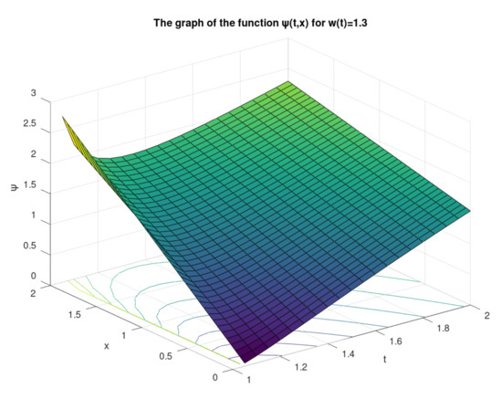
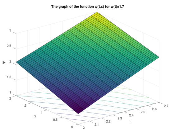
The graph of the function ψ for two values of the variable order $w\left(t\right)$ on the subintervals ${\mathbb{I}}_1$ and ${\mathbb{I}}_2$ are illustrated in Figure 1 and Figure 2.

Accordingly, we have

$$\begin{array}{ccc}\hfill {(logt)}^{\frac{1}{3}}|\psi (t,\mathrm{x})-\psi (t,{\mathrm{x}}^{*})|& =& \left|\frac{7}{5\sqrt{\pi }}{(logt)}^{\mathrm{w}\left(t\right)+\frac{1}{3}}+\frac{1}{t+1}\mathrm{x}\left(t\right)-\frac{7}{5\sqrt{\pi }}{(logt)}^{\mathrm{w}\left(t\right)+\frac{1}{3}}-\frac{1}{t+1}{\mathrm{x}}^{*}\left(t\right)\right|\hfill \\ & \le & \frac{1}{t+1}|\mathrm{x}\left(t\right)-{\mathrm{x}}^{*}\left(t\right)|\hfill \\ & \le & \frac{1}{2}|\mathrm{x}\left(t\right)-{\mathrm{x}}^{*}\left(t\right)|.\hfill \end{array}$$

Thus, the hypothesis (HP2) is valid with $g={\displaystyle \frac{1}{3}}$ and $\ell ={\displaystyle \frac{1}{2}}$.

By Equation $\left(15\right)$, the differential equation of the variable order Hadamard FBVP (14) is divided into two separate FDEs as follows

$$\left\{\begin{array}{c}{}^H{D}_{1^{+}}^{1.3}\mathrm{x}\left(t\right)={\displaystyle \frac{7}{5\sqrt{\pi }}}{(logt)}^{1.3}+{\displaystyle \frac{{(logt)}^{-\frac{1}{3}}}{t+1}}\mathrm{x}\left(t\right),t\in {\mathbb{I}}_1,\hfill \\ {}^H{D}_{1^{+}}^{1.7}\mathrm{x}\left(t\right)={\displaystyle \frac{7}{5\sqrt{\pi }}}{(logt)}^{1.7}+{\displaystyle \frac{{(logt)}^{-\frac{1}{3}}}{t+1}}\mathrm{x}\left(t\right),t\in {\mathbb{I}}_2.\hfill \end{array}\right.$$

For $t\in {\mathbb{I}}_1$, the variable order Hadamard FBVP (14) corresponds to the equivalent standard Hadamard FBVP

$$\left\{\begin{array}{c}{}^H{D}_{1^{+}}^{1.3}\mathrm{x}\left(t\right)={\displaystyle \frac{7}{5\sqrt{\pi }}}{(logt)}^{1.3}+{\displaystyle \frac{{(logt)}^{-\frac{1}{3}}}{t+1}}\mathrm{x}\left(t\right),t\in {\mathbb{I}}_1,\hfill \\ \mathrm{x}\left(1\right)=0,\mathrm{x}\left(2\right)=0.\hfill \end{array}\right.$$

(16)

Simply, one can check that condition (10) is fulfilled. Indeed,

$$\frac{2\ell [{(log{T}_1)}^{1-g}-{(log{T}_0)}^{1-g}]}{(1-g)\mathsf{\Gamma }\left({\mathrm{w}}_1\right)}{(log\frac{T_1}{T_0})}^{{\mathrm{w}}_1-1}=\frac{{(log2)}^{\frac{2}{3}}}{\left(\frac{2}{3}\right)\mathsf{\Gamma }\left(1.3\right)}{(log2)}^{0.3}\simeq 0.5279<1.$$

Let $\varphi \left(t\right)={(logt)}^{\frac{1}{2}}$. Hence,

$$\begin{array}{ccc}\hfill {}^H{I}_{1^{+}}^{{\mathrm{w}}_1}\varphi \left(t\right)& =& \frac{1}{\mathsf{\Gamma }\left(1.3\right)}{\int }_1^t{(log\frac{t}{s})}^{1.3-1}\frac{{(logs)}^{\frac{1}{2}}}{s}ds\hfill \\ & \le & \frac{1}{\mathsf{\Gamma }\left(1.3\right)}{\int }_1^t{(log\frac{t}{s})}^{0.3}\frac{1}{s}ds\hfill \\ & \le & \frac{0.75}{\mathsf{\Gamma }\left(2.3\right)}{(logt)}^{\frac{1}{2}}:={\lambda }_{\varphi \left(t\right)}\varphi \left(t\right).\hfill \end{array}$$

Therefore, the condition (HP3) is satisfied with $\varphi \left(t\right)={(logt)}^{\frac{1}{2}}$ and ${\lambda }_{\varphi \left(t\right)}={\displaystyle \frac{0.75}{\mathsf{\Gamma }\left(2.3\right)}}$.

By Theorem 3, the equivalent standard Hadamard FBVP (16) involves a solution ${\mathrm{x}}_1\in E_1$ uniquely, and from Theorem 4, the equivalent standard Hadamard FBVP (16) is Ulam–Hyers–Rassias stable.

On the other side, for $t\in {\mathbb{I}}_2$, the variable order Hadamard FBVP (14) can be rewritten as follows

$$\left\{\begin{array}{c}{}^H{D}_{1^{+}}^{1.7}\mathrm{x}\left(t\right)={\displaystyle \frac{7}{5\sqrt{\pi }}}{(logt)}^{1.7}+{\displaystyle \frac{{(logt)}^{-\frac{1}{3}}}{t+1}}\mathrm{x}\left(t\right),t\in {\mathbb{I}}_2\hfill \\ \mathrm{x}\left(2\right)=0,\mathrm{x}\left(e\right)=0.\hfill \end{array}\right.$$

(17)

Evidently,

$$\frac{2\ell [{(log{T}_2)}^{1-g}-{(log{T}_1)}^{1-g}]}{(1-g)\mathsf{\Gamma }\left({\mathrm{w}}_2\right)}{(log\frac{T_2}{T_1})}^{{\mathrm{w}}_2-1}=\frac{1-{(log2)}^{\frac{2}{3}}}{\left(\frac{2}{3}\right)\mathsf{\Gamma }\left(1.7\right)}{(log\frac{e}{2})}^{0.7}\simeq 0.0742<1.$$

Thus, the condition (10) is satisfied and

$$\begin{array}{ccc}\hfill {}^H{I}_{2^{+}}^{{\mathrm{w}}_2}\varphi \left(t\right)& =& \frac{1}{\mathsf{\Gamma }\left(1.7\right)}{\int }_2^t{(log\frac{t}{s})}^{1.7-1}\frac{{(logs)}^{\frac{1}{2}}}{s}ds\hfill \\ & \le & \frac{1}{\mathsf{\Gamma }\left(1.7\right)}{\int }_2^t{(log\frac{t}{s})}^{0.7}\frac{1}{s}ds\hfill \\ & \le & \frac{1}{\mathsf{\Gamma }\left(2.7\right)}{(logt)}^{\frac{1}{2}}:={\lambda }_{\varphi \left(t\right)}\varphi \left(t\right).\hfill \end{array}$$

This means that the condition (HP3) is fulfilled with $\varphi \left(t\right)={(logt)}^{\frac{1}{2}}$ and ${\lambda }_{\varphi \left(t\right)}={\displaystyle \frac{1}{\mathsf{\Gamma }\left(2.7\right)}}$.

By Theorem 3, the equivalent standard Hadamard FBVP (17) involves a solution ${\tilde{\mathrm{x}}}_2\in E_2$ uniquely, and from Theorem 4, we find that the variable order Hadamard FBVP (17) is Ulam–Hyers–Rassias stable. On the other side, it is known that

$${\mathrm{x}}_2\left(t\right)=\left\{\begin{array}{c}0,t\in {\mathbb{I}}_1,\hfill \\ {\tilde{\mathrm{x}}}_2\left(t\right),t\in {\mathbb{I}}_2.\hfill \end{array}\right.$$

As a result, by Definition 4, the variable order Hadamard FBVP (14) involves a solution uniquely in the format

$$\mathrm{x}\left(t\right)=\left\{\begin{array}{c}{\mathrm{x}}_1\left(t\right),t\in {\mathbb{I}}_1,\hfill \\ {\mathrm{x}}_2\left(t\right)=\left\{\begin{array}{c}0,t\in {\mathbb{I}}_1,\hfill \\ {\tilde{\mathrm{x}}}_2\left(t\right),t\in {\mathbb{I}}_2,\hfill \end{array}\right.\hfill \end{array}\right.$$

and, by Theorem 4, the variable order Hadamard FBVP (14) is Ulam–Hyers–Rassias stable.

5. Conclusions

In this paper, we introduced an abstract variable order boundary value problem of Hadamard FDEs with terminal conditions, where the function $\mathrm{w}\left(t\right):[1,T]\to (1,2]$ stands for the variable order of the given system. First, we reviewed some important specifications of Hadamard variable order operators and by an example, we showed that the semi-group property is not valid for variable order Hadamard integrals. Then, by defining a partition based on the generalized intervals, we introduced a piecewise constant function $\mathrm{w}\left(t\right)$ and converted the given variable order Hadamard FBVP (1) to an equivalent standard Hadamard BVP (6) of the fractional constant order. By using the standard fixed point theorems, we established the existence and uniqueness and, finally, the Ulam–Hyers–Rassias stability of its possible solutions was checked. Finally, using an example, we illustrated the theoretical findings.

References

- Riaz, U.; Zada, A.; Ali, Z.; Popa, I.L.; Rezapour, S.; Etemad, S. On a Riemann-Liouville type implicit coupled system via generalized boundary conditions. Mathematics 2021, 9, 1205. [Google Scholar] [CrossRef]
- Afshari, H.; Kalantari, S.; Karapinar, E. Solution of fractional differential equations via coupled fixed point. Electron. J. Differ. Equ. 2015, 286, 2015. [Google Scholar]
- Shah, K.; Hussain, W. Investigating a class of nonlinear fractional differential equations and its Hyers-Ulamstability by means of topological degree theory. Numer. Funct. Anal. Optim. 2019, 40, 1355–1372. [Google Scholar] [CrossRef]
- Boutiara, A.; Etemad, S.; Hussain, A.; Rezapour, S. The generalized U-H and U-H stability and existence analysis of a coupled hybrid system of integro-differential IVPs involving φ-Caputo fractional operators. Adv. Differ. Equ. 2021, 2021, 95. [Google Scholar] [CrossRef]
- Ben Chikh, S.; Amara, A.; Etemad, S.; Rezapour, S. On Hyers-Ulam stability of a multi-order boundary value problems via Riemann-Liouville derivatives and integrals. Adv. Differ. Equ. 2020, 2020, 547. [Google Scholar] [CrossRef]
- Mohammadi, H.; Rezapour, S.; Etemad, S.; Baleanu, D. Two sequential fractional hybrid differential inclusions. Adv. Differ. Equ. 2020, 2020, 385. [Google Scholar] [CrossRef]
- Etemad, S.; Rezapour, S.; Sakar, F.M. On a fractional Caputo-Hadamard problem with boundary value conditions via different orders of the Hadamard fractional operators. Adv. Differ. Equ. 2020, 2020, 272. [Google Scholar] [CrossRef]
- Amara, A.; Etemad, S.; Rezapour, S. Topological degree theory and Caputo-Hadamard fractional boundary value problems. Adv. Differ. Equ. 2020, 2020, 369. [Google Scholar] [CrossRef]
- Alsaedi, A.; Baleanu, D.; Etemad, S.; Rezapour, S. On coupled systems of time-fractional differential problems by using a new fractional derivative. J. Funct. Spaces 2016, 2016, 4626940. [Google Scholar] [CrossRef]
- Shah, K.; Khan, R.A. Existence and uniqueness results to a coupled system of fractional order boundary value problems by topological degree theory. Numer. Funct. Anal. Optim. 2016, 37, 887–899. [Google Scholar] [CrossRef]
- Etemad, S.; Souid, M.S.; Telli, B.; Kaabar, M.K.A.; Rezapour, S. Investigation of the neutral fractional differential inclusions of Katugampola-type involving both retarded and advanced arguments via Kuratowski MNC technique. Adv. Differ. Equ. 2021, 2021, 214. [Google Scholar] [CrossRef]
- Matar, M.M. Approximate controllability of fractional nonlinear hybrid differential systems via resolvent operators. J. Math. 2019, 2019, 8603878. [Google Scholar] [CrossRef]
- Thaiprayoon, C.; Sudsutad, W.; Alzabut, J.; Etemad, S.; Rezapour, S. On the qualitative analysis of the fractional boundary value problem describing thermostat control model via ψ-Hilfer fractional operator. Adv. Differ. Equ. 2021, 2021, 201. [Google Scholar] [CrossRef]
- Alzabut, J.; Ahmad, B.; Etemad, S.; Rezapour, S.; Zada, A. Novel existence techniques on the generalized ϕ-Caputo fractional inclusion boundary problem. Adv. Differ. Equ. 2021, 2021, 135. [Google Scholar] [CrossRef]
- Zada, A.; Ali, S. Stability analysis of multi-point boundary value problem for sequential fractional differential equations with noninstantaneous impulses. Int. J. Nonlinear Sci. Numer. Simul. 2018, 19, 763–774. [Google Scholar] [CrossRef]
- Zada, A.; Ali, S.; Li, Y. Ulam-type stability for a class of implicit fractional differential equations with non-instantaneous integral impulses and boundary condition. Adv. Differ. Equ. 2017, 2017, 317. [Google Scholar] [CrossRef] [Green Version]
- Agarwal, P.; Ammi, R.; Asad, J. Existence and uniqueness results on time scales for fractional nonlocal thermistor problem in the conformable sense. Adv. Differ. Equ. 2021, 2021, 162. [Google Scholar] [CrossRef]
- Agarwal, P.; Attary, M.; Maghasedi, M.; Kumam, P. Solving higher-order boundary and initial value problems via Chebyshev-spectral method: Application in elastic foundation. Symmetry 2020, 12, 987. [Google Scholar] [CrossRef]
- Sunarto, A.; Agarwal, P.; Sulaiman, J.; Chew, J.V.L.; Momani, S. Quarter-sweep preconditioned relaxation method, algorithm and efficiency analysis for fractional mathematical equation. Fractal Fract. 2021, 5, 98. [Google Scholar] [CrossRef]
- Wang, B.; Jahanshahi, H.; Volos, C.; Bekiros, S.; Yusuf, A.; Agarwal, P.; Aly, A.A. Control of a symmetric chaotic supply chain system using a new fixed-time super-twisting sliding mode technique subject to control input limitations. Symmetry 2021, 13, 1257. [Google Scholar] [CrossRef]
- Samko, S.G. Fractional integration and differentiation of variable order. Anal. Math. 1995, 21, 213–236. [Google Scholar] [CrossRef]
- Akgul, A.; Inc, M.; Baleanu, D. On solutions of variable-order fractional differential equations. Int. J. Opt. Control Theor. Appl. 2017, 7, 112–116. [Google Scholar] [CrossRef] [Green Version]
- Sun, H.G.; Chang, A.; Zhang, Y.; Chen, W. A review on variable-order fractional differential equations: Mathematical, foundations, physical models, and its applications. Fract. Calc. Appl. Anal. 2019, 22, 27–59. [Google Scholar] [CrossRef] [Green Version]
- Zhang, S. Existence of solutions for two point boundary value problems with singular differential equations of variable order. Electron. J. Differ. Equ. 2013, 245, 1–16. [Google Scholar]
- Zhang, S.; Hu, L. Unique existence result of approximate solution to initial value problem for fractional differential equation of variable order involving the derivative arguments on the half-axis. Mathematics 2019, 7, 286. [Google Scholar] [CrossRef] [Green Version]
- Refice, A.; Souid, M.S.; Stamova, I. On the boundary value problems of Hadamard fractional differential equations of variable order via Kuratowski MNC technique. Mathematics 2021, 9, 1134. [Google Scholar] [CrossRef]
- Bouazza, Z.; Etemad, S.; Souid, M.S.; Rezapour, S.; Martinez, F.; Kaabar, M.K.A. A study on the solutions of a multiterm FBVP of variable order. J. Funct. Spaces 2021, 2021, 9939147. [Google Scholar]
- Li, N.; Wang, C. New existence results of positive solution for a class of nonlinear fractional differential equations. Acta Math. Sci. 2013, 33, 847–854. [Google Scholar] [CrossRef]
- Sousa, J.V.D.C.; de Oliveira, E.C. Two new fractional derivatives of variable order with non-singular kernel and fractional differential equation. Comput. Appl. Math. 2018, 37, 5375–5394. [Google Scholar] [CrossRef]
- Lin, R.; Liu, F.; Anh, V.; Turner, I. Stability and convergence of a new explicit finite-difference approximation for the variable-order nonlinear fractional diffusion equation. Appl. Math. Comput. 2009, 212, 435–445. [Google Scholar] [CrossRef] [Green Version]
- Hristova, S.; Benkerrouche, A.; Souid, M.S.; Hakem, A. Boundary value problems of Hadamard fractional differential equations of variable order. Symmetry 2021, 13, 896. [Google Scholar] [CrossRef]
- Benchohra, M.; Lazreg, J.E. Existence and Ulam stability for nonlinear implicit fractional differential equations with Hadamard derivative. Stud. Univ. Babes-Bolyai Math. 2017, 62, 27–38. [Google Scholar] [CrossRef] [Green Version]
- Almeida, R.; Torres, D.F.M. Computing Hadamard type operators of variable fractional order. Appl. Math. Comput. 2015, 257, 74–88. [Google Scholar] [CrossRef] [Green Version]
- Almeida, R.; Tavares, D.; Torres, D.F.M. The Variable-Order Fractional Calculus of Variations, 1st ed.; Springer: Cham, Switzerland, 2019; ISBN 978-3-319-94005-2. [Google Scholar]
- Kilbas, A.A.; Srivastava, H.M.; Trujillo, J.J. Theory and Applications of Fractional Differential Equations, 1st ed.; Elsevier Science B.V.: Amsterdam, The Netherlands, 2006; ISBN 0444518320. [Google Scholar]
- An, J.; Chen, P. Uniqueness of solutions to initial value problem of fractional differential equations of variable-order. Dyn. Sys. Appl. 2019, 28, 607–623. [Google Scholar]
- Zhang, S. The uniqueness result of solutions to initial value problems of differential equations of variable-order. Rev. Real Acad. Cienc. Exactas Fis. Nat. Ser. A Mat. 2018, 112, 407–423. [Google Scholar] [CrossRef]
- Zhang, S.; Hu, L. The existence of solutions and generalized Lyapunov-type inequalities to boundary value problems of differential equations of variable order. AIMS Math. 2020, 5, 2923–2943. [Google Scholar] [CrossRef]
- Rus, I.A. Ulam stabilities of ordinary differential equations in a Banach space. Carpathian J. Math. 2010, 26, 103–107. [Google Scholar]
Publisher’s Note: MDPI stays neutral with regard to jurisdictional claims in published maps and institutional affiliations. |
© 2021 by the authors. Licensee MDPI, Basel, Switzerland. This article is an open access article distributed under the terms and conditions of the Creative Commons Attribution (CC BY) license (https://creativecommons.org/licenses/by/4.0/).