Article

On the Connectivity Measurement of the Fractal Julia Sets Generated from Polynomial Maps: A Novel Escape-Time Algorithm

1
School of Electrical Engineering and Automation, Qilu University of Technology (Shandong Academy of Science), Jinan 250353, China
2
Research Center of Dynamics System and Control Science, Shandong Normal University, Jinan 250014, China
*
Author to whom correspondence should be addressed.
Fractal Fract. 2021, 5(2), 55; https://doi.org/10.3390/fractalfract5020055
Submission received: 4 April 2021 / Revised: 8 June 2021 / Accepted: 8 June 2021 / Published: 13 June 2021
(This article belongs to the Section Numerical and Computational Methods)

Abstract

:
In this paper, a novel escape-time algorithm is proposed to calculate the connectivity’s degree of Julia sets generated from polynomial maps. The proposed algorithm contains both quantitative analysis and visual display to measure the connectivity of Julia sets. For the quantitative part, a connectivity criterion method is designed by exploring the distribution rule of the connected regions, with an output value C o in the range of [ 0 , 1 ] . The smaller the C o value outputs, the better the connectivity is. For the visual part, we modify the classical escape-time algorithm by highlighting and separating the initial point of each connected area. Finally, the Julia set is drawn into different brightnesses according to different C o values. The darker the color, the better the connectivity of the Julia set. Numerical results are included to assess the efficiency of the algorithm.

1. Introduction

Since the concept of fractals was proposed in the mid-1970s [1,2], it has gradually become an active research hotspot of nonlinear science. In recent years, the theoretical framework of fractals has become more and more mature [3,4,5]. At the same time, in order to explore the application of fractals in biology [6,7], physics [8,9], cryptography [10,11], and other fields, a lot of research and review have been carried out. As one of the important branches of fractal, the research on Julia sets can be traced back to the early 20th century, when French mathematician Gaston Julia [12] considered the characteristics of a simple complex map z n + 1 = z n 2 + c , z , c C in the case n . Due to the limitation of computer technology, the researchers at that time could not fully realize the complexity of the topology under such a simple iteration [13,14]. With the development of computer science, the two systematic works proposed by Mandelbrot have caused a new wave of research on the Mandelbrot set and the Julia set (M-J set for short). The study on algorithms to calculate the M-J sets provides visualization assistance for researchers to explore the internal structures and the dynamical behaviours. Among these algorithms, the escape-time algorithm [15], including the escape radius R and the maximum number of iterations N, is one of the most commonly used methods. Nowadays, a lot of research has been done on the improvement of E T A and proposal of other algorithms. In [16], the Mandelbrot set was displayed by a variety of colours to reveal patterns of finite attracting orbits. Liu et al. [17] proposed a new escape-time algorithm that could accelerate the construction process. Analogous study that reduces the iteration times can be seen in [9], which defined a kind of point as a no-escape point. Some follow-up studies are proposed for the Julia set construction algorithm of generalized polynomial mapping, z n + 1 = z n k + c , k N + [18,19]. Jovanovic presented a method to illustrate the Mandelbrot sets by analyzing the statistical information of the points’ calculation-paths [20]. By distinguishing the points with different colors according to the different strike frequency, the reference [21] presented an equipotential point algorithm to construct the Julia sets. Moreover, some research has been done to investigate the algorithm for constructing 3D M-J sets [22,23,24]. With the help of the E T A , some other related problems about the fractal have also been effectively analyzed and addressed. For instance, the E T A was well-adopted in an investigation on the computation of the Julia set’s dimension [25]. Based on the Julia set’s image generated by E T A , the authors proposed a novel image with visually meaningful cryptography, which has stronger anti-interference ability [26]. In [27], the dynamic behaviors of the network whose nodes are logistic maps was well-described by the M-J set formulated by E T A .
To further reveal the complex internal structure of the M-J set, some supplementary studies, including quantitative methods and visualization methods, were proposed and added to E T A [28,29,30,31,32,33,34,35]. For instance, by analyzing the trajectory of the critical points, Danca et al. [28,29] pointed out that the Julia set showed different connectivity by alternating the iteration of switched systems [30]. Afterwards, a kind of fractals paradox phenomenon “disconnected+disconnected=connected” and the corresponding graphical investigations were proposed in [31,32]. The Julia deviation distance method and Julia deviation plot method were given in the study of noise-perturbed Julia sets [34,35].
As mentioned above, although some progress has been made in the research of modifying the E T A to explore M-J sets’ properties, such as the bounded trajectories [20,21,28,29,36], symmetry property [19,22,24,31,32], and region location [9,17,18,24,33,34,35], few studies have been done on the connectivity measurement of M-J sets. For some high-order polynomial maps [29,31,37], the system generally has multiple critical points, which means that the parameter spaces of this type of map is more complicated than the classical Mandelbrot set. Therefore, the motivation of this work is to quantitatively and visually analyze the distribution of Julia’s connected regions. Therefore, the motivation of this work is to give the quantitative and visual analysis of the distribution law of connected regions for the Julia sets with diverse connectivity properties. The main novelties of this work can be summarized as follows:
(1)
This is the first attempt to solve the problem of measuring the connectivity of Julia sets generated from polynomial maps.
(2)
A criterion is designed to map the connectivity degree to the range of [ 0 , 1 ] . In this way, the quantification of connectivity degree is effectively achieved.
(3)
The connectivity is visualized by coloring Julia sets with different brightnesses, which provides an intuitive way to identify the connectivity degree.
The remainder of the paper is organized as follows. In Section 2, some definitions and preliminaries that will be used throughout the paper are presented. In Section 3, the frame of the proposed algorithm is given. Section 4 contains numerical results about a kind of switched system and a kind of quartic polynomial map. Quantitative analysis and visualization results are included in Section 4. In Section 5, the summation of this present work and prospects of future investigations are made.

2. Definitions and Preliminaries

Julia sets J ( f ) is defined as the closure of repelling periodic points of a complex function. That is, the trajectories of points in a Julia set remain bounded during the iterations of f. Particularly, if f has an attractive point w, the Julia set can be defined as J ( f ) = A ( w ) , where A ( w ) is the attractive domain of the attractive fixed point w [38,39]. The basic frame of E T A is mainly based on the following definition.
Definition 1.
Set ( x 0 , y 0 ) = z 0 C as an initial point of a complex map f. The filled Julia set of f is defined as
K ( f ) = { z 0 | f n ( z 0 ) , n } .
Julia set of f is the boundary of K ( f ) , t h a t i s , J ( f ) = K ( f ) .
The connectivity of the Julia set is determined by parameter c. For the classical map z n + 1 = z n 2 + c , z , c C , the set making J ( f ) connected, is named the Mandelbrot set, composed of all the cs that keep the trajectory of z 0 = 0 bounded.
As mentioned in the introduction, for some higher-order polynomial maps, the Julia sets present diverse connectivities according to the trajectories of critical points. In this paper, we use two such maps as examples to describe, verify the description of, and actually verify the proposed algorithm.
Example 1.
Danca et al.. [28,29] pointed out that Julia sets show different connectivities by studying a kind of switched map:
F 1 : z n + 1 = z n 2 + c 1 , if n is even , z n 2 + c 2 , if n is odd .
Same as Definition 1, the Julia set of system (1) is composed of z 0 , whose sequence is kept bounded. By analyzing the boundedness and periodicity of the two critical points 0 , c 1 , the following definition is given.
Definition 2.
The connectivity loci of system (1), denoted as M ( F ) , is separated into three parts, as follows:
(1) 
C L ( F ) denotes the locations of ( c 1 , c 2 ) ensuring the connectedness of J ( F ) .
(2) 
D L ( F ) denotes the locations of ( c 1 , c 2 ) ensuring the disconnectedness of J ( F ) .
(3) 
T D L ( F ) denotes the locations of ( c 1 , c 2 ) ensuring the totally disconnectedness of J ( F ) .
Example 2.
In [37], the authors investigated the connectivity of a polynomial map with degree d 2 . The work [37] contains the Julia sets from the following quartic map:
F 2 : z n + 1 = a ( z n + 2 ) 2 ( 3 z n 2 8 z n + 8 ) / 3 2 , a C .
Remark 1.
In [37], the authors denoted K ( F 2 ) as the F 2 ’s filled Julia set, I ( F 2 ) = C \ K ( F 2 ) as the escaping set. They pointed out that system (2) has three critical points 1 , 0 , 2 , whose relationship position with the two sets K ( F 2 ) , I ( F 2 ) determine the different connectivity of the corresponding Julia sets.

3. Escape-Time Algorithm Design

The purpose of the proposed algorithm is to quantify the connectivity of systems whose unconnected Julia sets have locally connected regions. Because connectivity is an opposite concept to fragmentation, the main idea of measuring connectivity is to find the relevant rules of fragment distribution. Details are as follows: The purpose of the proposed algorithm is to quantify the connectivity of systems whose unconnected Julia sets have locally connected regions. Because connectivity is an opposite concept to fragmentation, the main idea of measuring connectivity is to find the relevant rules of fragmentation distribution. Details are as follows:
(I)
First, similar to the classical E T A : for polynomial maps f, denote R,N as the escape radius and escape-time, respectively. For each point ( x 0 , y 0 ) in the lattice which contains J ( f ) , a serial number ( φ , ψ ) is assigned ( 1 φ , ψ M ) , where φ , ψ N + . M 2 is the image’s resolution.
(II)
Travel all ( φ , ψ ) in the range 1 φ , ψ M to get a set K based on the following rule: if | f n ( x 0 , y 0 ) | > R in which n N , the point ( φ , ψ ) is abandoned. Otherwise, ( φ , ψ ) K . The number of points in K is defined as n u m ( K ) .
(III)
In the set K, ψ and φ are iterated successively. Once a point ( φ , ψ ) is reached, we express it as ς p , 1 and regard it as the initial point of a connected region Ω p , 1 p M 2 .
(IV)
Each ς p , 1 = ( φ , ψ ) has, at most, eight neighbors in K. In counter-clockwise order, the eight points ( φ , ψ 1 ) , ( φ 1 , ψ 1 ) , ( φ 1 , ψ ) , ( φ 1 , ψ + 1 ) , ( φ , ψ + 1 ) , ( φ + 1 , ψ + 1 ) , ( φ + 1 , ψ ) , ( φ + 1 , ψ 1 ) are denoted as ς p , 2 , which means the second generation of ς p , 1 . Suppose that P 1 connected regions have been classified; then, all the points before the Q t h iteration (always in counter-clockwise order) of ς P , 1 are separated into a set K P , Q + , defined as
K P , Q + = l = 1 P 1 Ω p + q = 1 Q 1 ς p , q .
The Q t h iteration of ς P yields
Ω P ( Q t h i t e r a t i o n ) : { ς p , q } = : b a c k t o ( 3 ) . { ς p , q } : i n t o { Ω P } : i f ς p , q { K P , Q + } . i g n o r e : i f ς p , q { K P , Q + } . b a c k t o ( 3 ) : i f a l l ς p , q { K P , Q + } .
As shown in Figure 1, we illustrate a flowchart for a more intuitive explanation of the algorithm. The (a)–(c) parts of Figure 1 illustrate steps (I), (II), which are in accordance with the classical E T A .
The labelling process in steps (III), (IV) is shown in Figure 1d. Blue points in Figure 1d are the first points ς in regions Ω . The grey points labeled with several generations are those connected with ς . It can be seen from step (IV) that there are some redundant computations in the labelling process. Specifically, 43-times redundant computations occur in Figure 1d. To handle this problem, the linked storage structure illustrated in Figure 2 is adopted. In Figure 2, the white points depict ( φ , ψ ) that do not belong to the set K, and the black points are those that have been classified in the previous regions. The grey and blue ones are those that will be classified only in the set K P , Q ,
K P , Q = K l = 1 P 1 Ω p q = 1 Q 1 ς p , q .
(V)
Repeat steps (III) and (IV) until all points in K are classified. Count all the ς p , 1 in each region Ω and define the number as n u m ( C ) . It is clear that n u m ( C ) means the number of connected regions, that is, the degree of the fragmentation. Then, the connectivity criterion is defined as
C o ( J ) = n u m ( C ) n u m ( J ) : i f n u m ( C ) 1 , 0 : i f n u m ( C ) = 1 .
The two extreme cases of connectivity are shown in Figure 3. For the right-side case, the Julia set is totally disconnected; herein, C o ( J ) = 1 . For the left-side case, since there is a unique blue point ς 1 , 1 and a unique Ω 1 , we define C o ( J ) = 0 , which makes C o ( J ) change in the closed interval [0, 1]. The smaller the C o value, the better the connectivity.
(VI)
According to the value of C o , the color K ( F ) ranges from dark gray to light gray. Highlight and separate all the ς p , 1 with different colors.

4. Numerical Results

In this section, numerical results about Examples 1 and 2 are both given to illustrate the quantitative results and visual exhibitions. The parameters are given as R = 5 , N = 100 , M = 1000 .
For Example 1, the imaginary part of c 2 of system (1) is chosen as 0.3. The lattice for J ( F 1 ) is F 1 = [ 2 , 2 ] [ 2 , 2 ] . Figure 4a–c display 3 D and 2 D slices of M ( F ) . In Figure 4c, the dark-blue area denotes the connected locus C L ( F 1 ) , the light-blue area depicts the disconnected locus D L ( F 1 ) , and the remaining white area is the totally disconnected locus T D L ( F 1 ) . The corresponding filled Julia set constructed by the proposed algorithm with c 1 = 0.8 , c 2 = 0.32 + 0.3 i is illustrated in Figure 4d, in which the grey area is the filled Julia set K ( F 1 ) , and the blue points are the initial points ς p , 1 in each region Ω p .
The filled Julia sets corresponding with different parameters are separately illustrated in Figure 5. Point D is located in C L ( F 1 ) , and the other two points are located in D L ( F 1 ) . Point ( 0.9 , 0 ) is close to the edge of T D L ( F 1 ) . As can be seen from Figure 5, the darker the color, the better the connectivity of the Julia set. This law of the color gradient is consistent with the law of parameter distribution. The quantitative results about n u m ( C ) and C o ( J ) in Table 1 further support the above observations.
The results in Table 1 show that C o ( J ) can better explain the degree of connectivity than n u m ( C ) . The reason lies in the fact that the Julia set whose parameters are located close to T D L ( F 1 ) has fewer points, but more Ω regions.
To get a continuous distribution law of n u m ( C ) and C o ( J ) , two local enlarged regions of Figure 4b are given in Figure 4c and Figure 6, respectively. In the two enlarged regions, two intervals A C D L ( F 1 ) and E F D L ( F 1 ) are selected and derived into 100 points ( A : ( 0.95 , 0 ) , C : ( 0.752 , 0 ) , E : ( 0.4968 , 0.9326 ) , F : ( 0.576 , 0.992 ) ). Set M = 600 , and serial number 1–100 are assigned to those points, in which C and E correspond to serial number 1.
In Table 2 and Table 3, we list part of the n u m ( C ) and C o ( J ) in two intervals.
In order to visualize the changing rule of n u m ( C ) and C o ( J ) , Figure 7 shows the curve and bar graph of the whole 100 points.
Figure 7 has dual longitudinal axes, which contains blue N u m ( c ) on the left side, and red C o ( J ) on the right side. The results in Table 2 and Table 3 and Figure 7 further verify that C o ( J ) can explain the degree of connectivity better than n u m ( C ) . In Figure 7, the change of n u m ( C ) is not obvious, but it decreases sharply when the parameter is close to T D L ( F 1 ) . This is because when the parameters are close to T D L ( F ) , the main structure of K ( F 1 ) almost disappears. The C o ( J ) presents the exponential growth rule when the parameter point tends to T D L ( F 1 ) . These results testify the effectiveness of our algorithm.
For Example 2, we first give the parameter space of the system (2) in Figure 8, which is calculated based on the bounded trajectory of one of the three critical points (this picture has been shown in Figure 8 in [37]). As the Figure 8 shows, the light-blue set is composed of all parameter a, which ensure that the trajectory of critical point 1 is bounded. Based on the research in [37], the Julia set corresponds to any point in Figure 8 which may have a disconnected structure. Therefore, three points marked as G , H , I were chosen to illustrate the corresponding Julia sets.
Three Julia sets generated by points G , H , I are shown in Figure 8. In Figure 8, the Julia sets of points I can be referred to [37]; meanwhile, the Julia sets of points G , H are newly added in this work. Through the new proposed algorithm, three Julia sets present the colors matching with their connectivity’s degrees. Simulation results of system (2) further verify the effectiveness of the proposed algorithm Figure 9.

5. Conclusions

The Julia set is one of the most important topics in the field of fractals. With the aid of computer simulation, the research of constructing M-J sets has gradually become a research hotspot. The most basic algorithm to calculate the M J sets is the escape-time algorithm.
This work focused on the modification of the classical E T A by considering the measurement of the connectivity of Julia sets. By calculating the ratio of fragmentation regions’ numbers to the whole points’ numbers in K, a connectivity criterion C o was constructed to quantize the degree of connectivity. The visualization of the Julia set is also improved by highlighting the initial points of each connected region and distinguishing the brightness of K according to different C o . The numerical results of two kinds of polynomial maps are given to illustrate the realization process of the proposed algorithm.
Note that the main idea of the proposed algorithm is to find the relevant rules of fragmentation distribution. It is of interest to explore the relationship between the connectivity criterion and the resolution. The change curves of n u m ( C ) and C o ( J ) in the interval A C (we take the same 20 points as in Table 2) have been demonstrated in Figure 10. The results illustrate general trends, such as that n u m ( C ) increases with the increase of M, and C o ( J ) decreases with the increase of M. However, Julia sets with different parameters have somewhat different changing rules with the increase of M. Therefore, it is difficult to summarize a general convergence rule. Thus, there is still much work that needs to be further investigated.

Author Contributions

Y.Z. (Yang Zhao): Conceptualization, writing, editing and methodology. S.Z.: Software, editing. Y.Z. (Yi Zhang): Investigation, validation. D.W.: Review, editing and supervision. All authors have read and agreed to the published version of the manuscript.

Funding

This research received no external funding.

Institutional Review Board Statement

Not applicable.

Informed Consent Statement

Not applicable.

Data Availability Statement

Data sharing is not applicable to this article.

Acknowledgments

The research is supported by the Program of National Natural Science Foundation of China (No. 61703251), the China Postdoctoral Science Foundation Funded Project (No. 2017M612337), and the Scientific and Technological Planning Projects of Universities in Shandong Province (No. J18KB097).

Conflicts of Interest

The authors declare no conflict of interest with any editor, reviewer, etc. of the journal.

References

  1. Peitgen, H.O.; Richter, P.H. The Beauty of Fractals; Springer: Berlin/Heidelberg, Germany, 1986. [Google Scholar]
  2. Mandelbrot, B.B. The Fractal Geometry of Nature; WH Freeman: New York, NY, USA, 1982. [Google Scholar]
  3. Hutchinson, J.E. Fractals and self similarity. Indiana Univ. Math. J. 1981, 30, 713–747. [Google Scholar] [CrossRef]
  4. Barnsley, M.F. Fractals Everywhere; Academic Press: Boston, MA, USA, 1988. [Google Scholar]
  5. Blankers, V.; Rendfrey, T.; Shukert, A.; Shipman, P.D. Julia and Mandelbrot Sets for Dynamics over the Hyperbolic Numbers. Fractal Fract. 2019, 3, 6. [Google Scholar] [CrossRef] [Green Version]
  6. Losa, G.A. Fractals in biology and medicine. In Reviews in Cell Biology and Molecular Medicine; Birkhäuser: Locarno, Switzerland, 2006. [Google Scholar]
  7. Pickover, C.A. Biom orphs: Computer displays of biological forms generated from mathematical feedback loops. In Computer Graphics Forum; Blackwell Publishing Ltd.: Oxford, UK, 1986; Volume 5, pp. 313–316. [Google Scholar]
  8. Bercioux, D.; Iñiguez, A. Quantum fractals. Nat. Phys. 2019, 15, 111–112. [Google Scholar] [CrossRef]
  9. Wang, X.Y.; Liu, W.; Yu, X.J. Research on Brownian movement based on generalized Mandelbrot–Julia sets from a class complex mapping system. Mod. Phys. Lett. B 2007, 21, 1321–1341. [Google Scholar] [CrossRef]
  10. Ortiz, S.M.; Parra, O.; Miguel, J.; Espitia, R. Encryption through the Use of Fractals. Int. J. Math. Anal. 2017, 11, 1029–1040. [Google Scholar] [CrossRef]
  11. Sun, Y.Y.; Xu, R.D.; Chen, L.N.; Hu, X.P. Image compression and encryption scheme using fractal dictionary and Julia set. IET Image Process. 2015, 9, 173–183. [Google Scholar] [CrossRef]
  12. Julia, G. Mémoire sur l’itération des fonctions rationnelles. J. Math. Pures Appl. 1918, 8, 47–245. [Google Scholar]
  13. Fatou, P. Sur les équations fonctionnelles. Bull. De La Société Mathématique De Fr. 1919, 47, 161–271. [Google Scholar]
  14. Smale, S. Differentiable dynamical systems. Bull. Am. Math. Soc. 1967, 73, 747–817. [Google Scholar] [CrossRef] [Green Version]
  15. Barnsley, M.F.; Devaney, R.L.; Mandelbrot, B.B.; Peitgen, H.O.; Saupe, D. The Science of Fractal Images; Springer: New York, NY, USA, 1988. [Google Scholar]
  16. Welstead, S.T.; Cromer, T.L. Coloring periodicities of two-dimensional mappings. Comput. Graph. 1989, 13, 539–543. [Google Scholar] [CrossRef]
  17. Liu, X.D.; Zhu, Z.L.; Wang, G.X.; Zhu, W.Y. Composed accelerated escape-time algorithm to construct the general Mandelbrot sets. Fractals 2001, 9, 149–153. [Google Scholar] [CrossRef]
  18. Liu, S.; Cheng, X.C.; Fu, W.H.; Zhou, Y.P.; Li, Q.Z. Numeric characteristics of generalized M-set with its asymptote. Appl. Math. Comput. 2014, 243, 767–774. [Google Scholar] [CrossRef]
  19. Liu, M.; Liu, S.; Fu, W.; Zhou, J. Distributional escape-time algorithm based on generalized fractal sets in cloud environment. Chin. J. Electron. 2015, 24, 124–127. [Google Scholar] [CrossRef]
  20. Jovanovic, P.; Tuba, M.I.; Simian, D.A.; Romania, S.S. A new visualization algorithm for the Mandelbrot set. In Proceedings of the 10th WSEAS International Conference on Mathematics and Computers in Biology and Chemistry; World Scientific and Engineering Academy and Society (WSEAS): Stevens Point, WI, USA, 2009; pp. 162–166. [Google Scholar]
  21. Sun, Y.Y.; Hou, K.N.; Zhao, X.D.; Lu, Z.X. Research on characteristics of noise-perturbed M-J sets based on equipotential point algorithm. Commun. Nonlinear Sci. Numer. Simul. 2016, 30, 284–298. [Google Scholar] [CrossRef] [Green Version]
  22. Sun, Y.Y.; Wang, X.Y. Quaternion M set with none zero critical points. Fractals 2009, 17, 427–439. [Google Scholar] [CrossRef]
  23. Sun, Y.Y.; Wang, X.Y. Noise-perturbed quaternionic Mandelbrot sets. Int. J. Comput. Math. 2009, 86, 2008–2028. [Google Scholar] [CrossRef]
  24. Martineau, É.; Rochon, D. On a bicomplex distance estimation for the Tetrabrot. Int. J. Bifurc. Chaos 2005, 15, 3039–3050. [Google Scholar] [CrossRef]
  25. Mohammed, A.J. A comparison of fractal dimension estimations for filled Julia fractal sets based on the escape-time algorithm. In AIP Conference Proceedings; AIP Publishing LLC: Malang, Indonesia, 2019; Volume 2086, p. 030026. [Google Scholar]
  26. Wang, H.X.; Zhao, X.F.; Shi, Y.Q.; Kim, H.J.; Piva, A. Digital Forensics and Watermarking; Springer Nature: Chengdu, China, 2019. [Google Scholar]
  27. Rǎdulescu, A.; Pignatelli, A. Real and complex behavior for networks of coupled logistic maps. Nonlinear Dyn. 2017, 87, 1295–1313. [Google Scholar] [CrossRef] [Green Version]
  28. Danca, M.F.; Romera, M.; Pastor, G. Alternated Julia sets and connectivity properties. Int. J. Bifurc. Chaos 2009, 19, 2123–2129. [Google Scholar] [CrossRef] [Green Version]
  29. Danca, M.F.; Bourke, P.; Romera, M. Graphical exploration of the connectivity sets of alternated Julia sets. Nonlinear Dyn. 2013, 73, 1155–1163. [Google Scholar] [CrossRef] [Green Version]
  30. Zhang, Y.X. Switching-induced Wada basin boundaries in the Héon map. Nonlinear Dyn. 2013, 73, 2221–2229. [Google Scholar] [CrossRef]
  31. Wang, D.; Liu, S.T. On the boundedness and symmetry properties of the fractal sets generated from alternated complex map. Symmetry 2016, 8, 7. [Google Scholar] [CrossRef] [Green Version]
  32. Wang, D.; Liu, S.T.; Zhao, Y. A preliminary study on the fractal phenomenon: Disconnected+disconnected=connected. Fractals 2017, 25, 1750004. [Google Scholar] [CrossRef]
  33. Andreadis, I.; Karakasidis, T.E. On a numerical approximation of the boundary structure and of the area of the Mandelbrot set. Nonlinear Dyn. 2015, 80, 929–935. [Google Scholar] [CrossRef]
  34. Andreadis, I.; Karakasidis, T.E. On a topological closeness of perturbed Julia sets. Appl. Math. Comput. 2010, 217, 2883–2890. [Google Scholar] [CrossRef]
  35. Andreadis, I.; Karakasidis, T.E. On a closeness of the Julia sets of noise-perturbed complex quadratic maps. Int. J. Bifurc. Chaos 2012, 22, 1250221. [Google Scholar] [CrossRef]
  36. Jovanovic, R.; Tuba, M. A visual analysis of calculation-paths of the Mandelbrot set. WSEAS Trans. Comput. 2009, 8, 1205–1214. [Google Scholar]
  37. Katagata, K. Quartic Julia sets including any two copies of quadratic Julia sets. Discret. Contin. Dyn. Syst. 2016, 36, 2103. [Google Scholar] [CrossRef] [Green Version]
  38. Sajid, M.; Kapoor, G.P. Chaos in dynamics of a family of transcendental meromorphic functions. J. Nonlinear Anal. Appl. 2017, 2017, 1–11. [Google Scholar] [CrossRef] [Green Version]
  39. Sajid, M. Bifurcation and chaos in real dynamics of a two-parameter family arising from generating function of generalized Apostol-type polynomials. Math. Comput. Appl. 2018, 23, 7. [Google Scholar] [CrossRef]
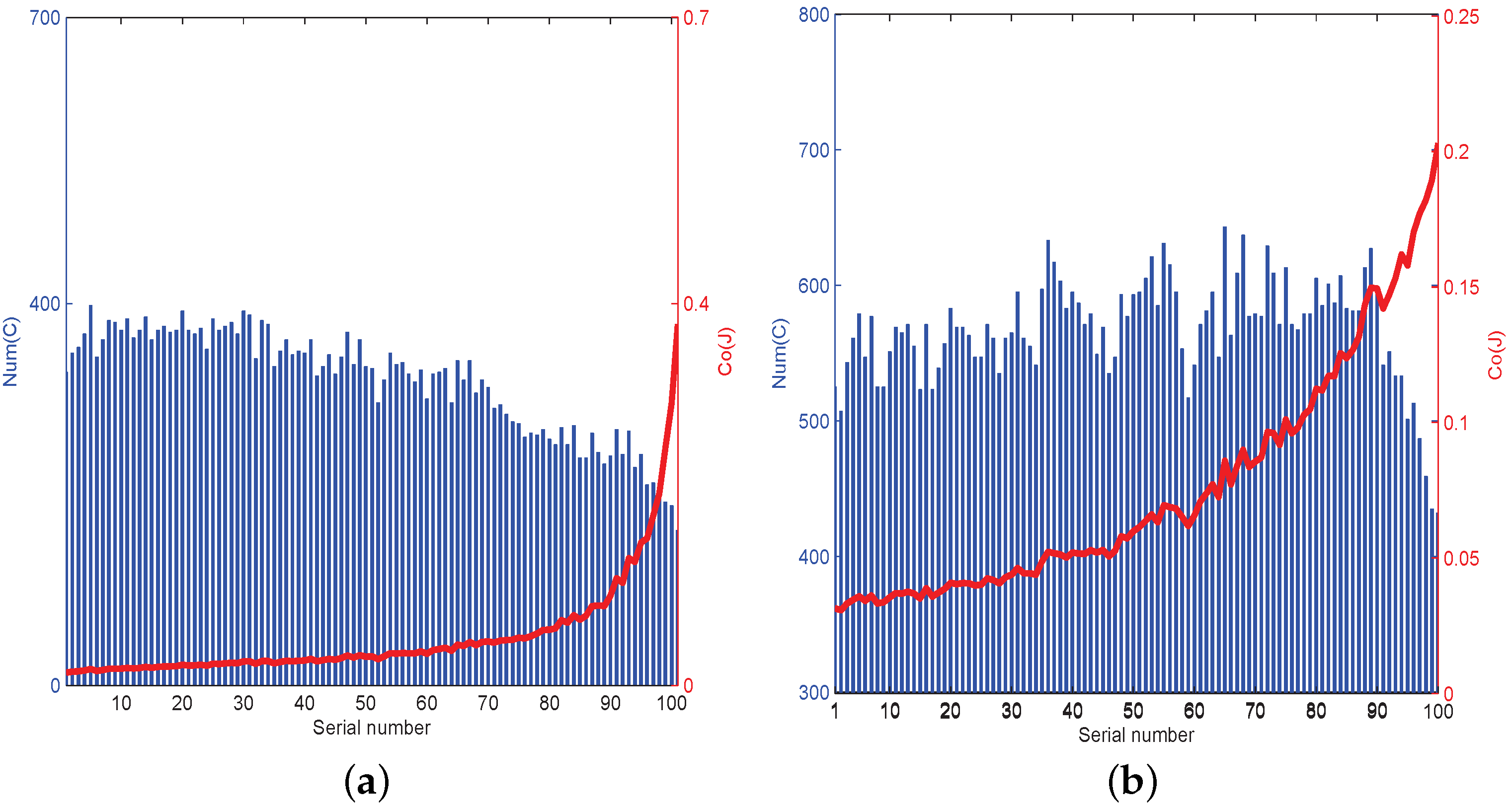
 [Green Version]
Figure 1. The flowchart of the proposed algorithm in which (a,b): corresponding to the steps (I), (II). (c,d): corresponding to the steps (III), (IV). (e,f): corresponding to the step (V).
Fractalfract 05 00055 g001
Figure 2. The labelling process in step (IV).
Fractalfract 05 00055 g002
Figure 3. Two extreme two cases of steps (IV), (V).
Fractalfract 05 00055 g003
Figure 4. (a) The spatial C L ( F 1 ) with I m ( c 2 ) = 0.3 ( I m is the imaginary part). (b) The 2 D slice of M ( F ) I m ( c 2 ) = 0.3 with R e ( c 2 ) = 0.32 . ( R e is the real part). (c) The local enlarged region of (b). (d) The filled Julia set K ( F 1 ) with B point parameter c 1 = 0.8 .
Fractalfract 05 00055 g004
Figure 5. The filled Julia sets of system F 1 with different brightness based on C o . (a) c 1 = 0.68 , c 2 = 0.32 + 0.3 i , (c) c 1 = 0.8 , c 2 = 0.32 + 0.3 i , (e) c 1 = 0.9 , c 2 = 0.32 + 0.3 i . (b,d,f): Separate the points ς p , 1 corresponding to (a,c,e).
Fractalfract 05 00055 g005
Figure 6. The local enlarged region of Figure 4b.
Fractalfract 05 00055 g006
Figure 7. The n u m ( C ) and C o ( J ) in: (a) A C , (b) E F .
Fractalfract 05 00055 g007
Figure 8. The parameter space of system (2). The light-blue region is the set of parameter a, such that { a C : F 2 n ( z 0 = 1 ) , n } [37].
Fractalfract 05 00055 g008
Figure 9. The filled Julia sets of system F 2 with different brightnesses based on C o . (a) a = 0.3 + 0.02 i , (c) a = 0.324 + 0.01 i , (e). a = 1 / 3 + 83 i / 2000 . (b,d,f): Separate the points ς p , 1 corresponding to (a,c,e).
Fractalfract 05 00055 g009
Figure 10. (a) The change curve of n u m ( C ) with the increase of M. (b) The change curve of C o ( J ) with the increase of M.
Fractalfract 05 00055 g010
Table 1. n u m ( C ) and C o ( J ) of the three cases in Figure 5.
J ( F ) Figure 5aFigure 5bFigure 5c
n u m ( C ) 1372260
C o ( J ) 00.02240.0492
Table 2. n u m ( C ) and C o ( J ) in the interval A C .
No.15101520253035404550
n u m ( C ) 348344384372372372388350362344332
C o ( J ) 0.01430.01510.01830.01920.02070.02240.02520.02450.02760.02860.0303
No.556065707580859095100-
n u m ( C ) 338326320290260252238268210162-
C o ( J ) 0.03390.03700.04120.04470.04920.05970.07290.11210.15420.3785-
Table 3. n u m ( C ) and C o ( J ) in the interval E F .
No.15101520253035404550
n u m ( C ) 311299317319311349395397363411439
C o ( J ) 0.01940.01930.02130.02240.02290.02710.03220.03470.03380.04150.0484
No.556065707580859095100-
n u m ( C ) 371445371423429391417381349321-
C o ( J ) 0.04500.05940.05480.06970.07970.08300.10400.12020.17070.2967-
Publisher’s Note: MDPI stays neutral with regard to jurisdictional claims in published maps and institutional affiliations.

