Continuity Result on the Order of a Nonlinear Fractional Pseudo-Parabolic Equation with Caputo Derivative

Abstract

In this paper, we consider a problem of continuity fractional-order for pseudo-parabolic equations with the fractional derivative of Caputo. Here, we investigate the stability of the problem with respect to derivative parameters and initial data. We also show that $u_{{\omega }^{\prime }}\to u_{\omega }$ in an appropriate sense as ${\omega }^{\prime }\to \omega$, where $\omega$ is the fractional order. Moreover, to test the continuity fractional-order, we present several numerical examples to illustrate this property.

1. Introduction

Fractional PDEs are of considerable significance in different fields, such as memory effect physics and engineering, viscoelasticity, porous media, etc. [1,2,3,4,5,6,7,8,9,10,11,12,13,14,15] and C. Cattani in [16,17,18]. Viscosity is of particular significance in the study of the mechanical properties of structures and biological materials. Recently, many researchers applied fractional calculations to probe the viscosity of such materials with high accuracy. Fraction PDEs are the main tool solving that phenomena model.

In this work, we focus on the time-fractional pseudo-parabolic equation as follows

$$\left\{\begin{array}{cc}{\partial }_t^{\omega }\left(u(x,t)+\kappa \mathcal{R}u(x,t)\right)+\mathcal{R}u(x,t)=\mathcal{G}((x,t,u(x,t)),\hfill & (x,t)\in \mathsf{\Omega }\times (0,T],\hfill \\ u(x,t)=0,\hfill & (x,t)\in \partial \mathsf{\Omega }\times (0,T],\hfill \\ u(x,0)=g_0\left(x\right),\hfill & x\in \mathsf{\Omega },\hfill \\ u_t(x,0)=0,\hfill & x\in \mathsf{\Omega },\hfill \end{array}\right.$$

(1)

where $\mathsf{\Omega }$ is a bounded domain in $R^n$ with sufficiently smooth boundary $\partial \mathsf{\Omega }$, $1<\omega <2$ and the Caputo fractional derivative operator of order $\omega$ is given by the notation as ${\partial }_t^{\omega }$. Assume that the function u is definitely continuous in time, then the definition in [19] make less to the traditional form

$${\partial }_t^{\omega }u(x,t)=\frac{1}{\mathsf{\Gamma }(2-\omega )}{\int }_0^t{(t-s)}^{1-\omega }\frac{{\partial }^{2}u(x,s)}{ds}ds,$$

(2)

where $\frac{{\partial }^{2}u}{ds}$ is the second order integer derivative of function $u\left(s\right)$ with respect to the independent variable s and $\mathsf{\Gamma }$ is the Gamma function. The operator $\mathcal{R}$ is defined in Section 2.2. Some functions $\mathcal{G},g_0\left(x\right)$ are defined later. The Equation (1) defines the mechanism of mass transfer in fractal arrangement structures.

In case $\omega =1$ with the derivative of integer order, the problem (1) becomes the well known pseudo-parabolic as follows

$$u_t+\kappa \mathcal{R}{u}_t+\mathcal{R}u=\mathcal{G}\left(u\right).$$

(3)

The Equation (3) is called the pseudo-parabolic, which has many real-world applications, a case in this point is that the seepage of homogeneous fluids from a broken rock, unidirectional distribution of long waves of nonlinear dispersion [20,21] and Population aggregation [22] (where u is the population density). Moreover, there are a lot of works on well-posedness of the pseudo-parabolic equation with classical derivative, for instance, we can see in [23,24,25,26,27,28,29,30,31,32,33,34,35] and the references therein. In particular, in fractional calculus, investigating the existence, uniqueness, stability of fractional differential equations, has been the important goal in the scientific community. To the best of our knowledge, there are a few papers which consider the fractional-order of the pseudo-parabolic partial differential equation. Recently, the authors in [36] generalized Ulam-Hyers-Rassias’s stability results for FPPDE solution. M. Beshtokov [37,38,39] considered a boundary value problem for FPPDE. However, the regularity of mild solutions for FPPDE has not been investigated.

It follows that continuity of the solutions with respect to these parameters is important for modeling purposes. This paper comes from the motivation of [40] for considering the continuity of the solutions on fractional order. In practical problem, the parameter is defined or computed by experiments. Therefore, we only know its value incorrectly. Even if the parameters are known exactly but are irrational, then we also get only its approximate value. Assume that ${\omega }^{\prime }\to \omega$, a natural question is as follows

$$\mathrm{Does}{u}_{{\omega }^{\prime }}\to u_{\omega }\mathrm{in}\mathrm{an}\mathrm{appropriate}\mathrm{sense}\mathrm{as}{\omega }^{\prime }\to \omega ?$$

(4)

The main purpose of our paper is answer above question. The difficulty in the problem occurs when we have to evaluate the upper and lower quantities by the terms independent of fractional order $\alpha$. The question (4) for linear fractional wave equation has been recent studied in [41]. Due to the nonlocal and nonlinearity of our problem, we have to choose an effective method to give suitable estimation.

This paper is organized as follows. Section 2 shows the premilinaries of the Mittag-Leffler function and mild solution. The key findings are discussed in Section 3 which demonstrates the continuous dependency of the problem solution (1) on input data and the fractional parameter. In the last section, we show some numerical examples to illustrate the property which is called that the continuity fractional-order.

2. Preliminaries

2.1. The Mittag-Leffler Function

The Mittag-Leffler function is denoted and defined as following

$$\begin{array}{c}\hfill E_{\omega ,\varphi }\left(\xi \right)=\sum _{n=1}^{\infty }\frac{{\xi }^n}{\mathsf{\Gamma }(n\omega +\varphi )},\xi \in \mathbb{C},\end{array}$$

for $\omega >0$ and $\varphi \in \mathbb{R}$. We recall the following lemmas (we can see in [7,42,43]), that would be helpful for the primary analysis of Section 3 and Section 4.

Lemma 1.

If $1<\omega <2$, with for all $\xi >0$ and $\mathcal{C}$ is a positive number which only depends on ω, such that

$$\begin{array}{c}\hfill |E_{\omega ,1}(-\xi )|\le \mathcal{C},|E_{\omega ,\omega }(-\xi )|\le \mathcal{C}.\end{array}$$

Lemma 2.

For $\lambda >0$ the following identities holds true

$$\begin{array}{cc}\hfill & {\partial }_{\xi }{E}_{\omega ,1}(-\lambda {\xi }^{\omega })=-\lambda {\xi }^{\omega -1}{E}_{\omega ,\omega }(-\lambda {\xi }^a),\hfill \\ \hfill & {\partial }_{\xi }\left({\xi }^{\omega -1}{E}_{\omega ,\omega }(-\lambda {\xi }^{\omega })\right)={\xi }^{\omega -2}{E}_{\omega ,\omega -1}(-\lambda {\xi }^{\omega }),\hfill \end{array}$$

(5)

where ξ is a positive real number.

Proof. 

We can use Lemma 2.2 in [41] to prove the above Lemma. □

Lemma 3.

Assume $1<\omega <2$ and if T is a number that large enough then we get

$$\begin{array}{c}\hfill E_{\omega ,1}(-{\lambda }_j{T}^{\omega })\ne 0.\end{array}$$

(6)

For all j is a natural number, there are always two constants: ${\mathcal{C}}^1\omega$ and ${\mathcal{C}}^2\omega$ such that

$$\begin{array}{c}\hfill \frac{{\mathcal{C}}_{\omega }^1}{1+{\lambda }_j{T}^a}\le \left|E_{\omega ,1}(-{\lambda }_j{T}^a)\right|\le \frac{{\mathcal{C}}_{\omega }^2}{1+{\lambda }_j{T}^{\omega }}.\end{array}$$

(7)

Proof. 

This Lemma can be found in [44]. □

From Lemma $2.3$ in [40], we have the following Lemmas.

Lemma 4.

Let $1<\sigma <\nu <2$ and $\omega \in (\sigma ,\nu )$. There exist positive constants ${\mathcal{C}}_1$, ${\mathcal{C}}_2$, ${\mathcal{C}}_3$ which only depend on $\sigma ,\nu$ such that for any $\xi >0$ we get

$$\begin{array}{c}\hfill \frac{{\mathcal{C}}_1(\sigma ,\nu )}{1+\xi }\le |E_{\omega ,1}(-\xi )|\le \frac{{\mathcal{C}}_2(\sigma ,\nu )}{1+\xi },\left|E_{\omega ,\omega }(-\xi )\right|\le \frac{{\mathcal{C}}_3(\sigma ,\nu )}{1+\xi }.\end{array}$$

(8)

Lemma 5.

Let $0<\xi \le T$ and $0<\sigma <\omega <{\omega }^{\prime }<\nu$. For every $ϵ>0$ that independent of ω, there always exists ${\mathcal{C}}_{ϵ}$ such that

$$\begin{array}{c}\hfill |{\xi }^{\omega }-{\xi }^{{\omega }^{\prime }}|\le max(T^{\nu +2ϵ},1){\mathcal{C}}_{ϵ}{({\omega }^{\prime }-\omega )}^{ϵ}{T}^{\omega -ϵ}.\end{array}$$

(9)

Proof. 

We can find it in Lemma $3.2$ [41]. □

We have the following lemmas by applying Lemmas $3.3$ and $3.4$ from Section 3 [41].

Lemma 6.

Assume that $ϵ>0.$ and $1<\sigma <\omega <{\omega }^{\prime }<\nu <2.$ Then there is a positive constant ${\mathcal{D}}_1(\sigma ,\nu ,ϵ,\rho ,T)$, such that

$$\begin{array}{cc}\hfill & |E_{\omega ,1}(-{\lambda }_n{\xi }^{\omega })-E_{{\omega }^{\prime },1}(-{\lambda }_n{\xi }^{{\omega }^{\prime }})|\hfill \\ \hfill & \le {\mathcal{D}}_1(\sigma ,\nu ,ϵ,\rho ,T){\lambda }_n^{\rho -1}{t}^{-\nu (1-\rho )-ϵ}\left[{({\omega }^{\prime }-\omega )}^{ϵ}+({\omega }^{\prime }-\omega )\right],\hfill \end{array}$$

(10)

where $0\le \rho \le 1$ and $0<\xi \le T.$

Proof. 

Using Lemma 3.3 from Section 3 in [41] to prove above Lemma. □

Lemma 7.

Assume that $1<\sigma <\omega <{\omega }^{\prime }<\nu <2$. For any $ϵ>0$ and $0\le \rho \le 1$ then there is a positive number ${\mathcal{D}}_2(\sigma ,\nu ,ϵ,\rho ,T)$ which is independent of ω and ${\omega }^{\prime }$ such that the following

$$\begin{array}{cc}\hfill |{\xi }^{\omega -1}{E}_{\omega ,\omega }(-{\lambda }_n{\xi }^{\omega })& -{\xi }^{{\omega }^{\prime }-1}{E}_{{\omega }^{\prime },{\omega }^{\prime }}(-{\lambda }_n{t}^{{\omega }^{\prime }})|\hfill \\ \hfill & \le {\mathcal{D}}_2(\sigma ,\nu ,ϵ,\rho ,T){\lambda }_n^{\rho -1}{t}^{\sigma \rho -ϵ-1}\left[{({\omega }^{\prime }-\omega )}^{ϵ}+({\omega }^{\prime }-\omega )\right].\hfill \end{array}$$

(11)

Proof. 

Applying Lemma $3.4$ in [41] to prove this Lemma. □

2.2. Related Notation and Representation of the Solution

We introduce some of the necessary Sobolev spaces and correct some notation. Note ${\mathbb{L}}^2\left(\mathsf{\Omega }\right),H_0^1\left(\mathsf{\Omega }\right),H^2\left(\mathsf{\Omega }\right)$ denote the normal spaces of Sobolev. The symmetrical, uniform elliptical operator $\mathcal{R}:{\mathbb{L}}^2\left(\mathsf{\Omega }\right)\to {\mathbb{L}}^2\left(\mathsf{\Omega }\right)$ is defined by

$$\begin{array}{c}\hfill \mathcal{R}\mathbf{w}\left(s\right)=r\left(s\right)\mathbf{w}(s,t)-\sum _{m=1}^n{\frac{\partial }{\partial s}}_m\left({\mathcal{R}}_{mk}\left(s\right)\frac{\partial }{\partial s_k}\mathbf{w}\left(s\right)\right),s\in \overline{\mathsf{\Omega }},\end{array}$$

where $D\left(\mathcal{R}\right)=H_0^1\left(\mathsf{\Omega }\right)\cap H^2\left(\mathsf{\Omega }\right)$. With assumption $r\left(s\right)\in C(\overline{\mathsf{\Omega }},[0,\infty )$, ${\mathcal{R}}_{mk}\in C^1\left(\overline{\mathsf{\Omega }}\right),{\mathcal{R}}_{mk}={\mathcal{R}}_{km}$, $1\le m,k\le n,$ and there exist a positive constant $\tilde{R}>0$, for $x\in \overline{\mathsf{\Omega }},\eta =({\eta }_1,{\eta }_2,\cdots ,{\eta }_n)\subset {\mathbb{R}}^n$, such that

$$\tilde{R}\sum _{i=1}^n{\eta }_i^2\le \sum _{1\le m,k\le n}{\eta }_i{\mathcal{R}}_{mk}\left(x\right){\mu }_k.$$

We can search the above point in [45]. Now let us recall that the spectral problem

$$\begin{array}{c}\hfill \mathcal{R}{\psi }_n\left(x\right)={\lambda }_n{\psi }_n\left(x\right)\mathrm{in}\mathsf{\Omega }\mathrm{and}{\psi }_n\left(x\right)=0\mathrm{on}\partial \mathsf{\Omega }\end{array}$$

(12)

admits a family of eigenvalues (see, e.g., [46])

$$0<{\lambda }_1\le {\lambda }_2\le {\lambda }_3\le ...\le {\lambda }_n\le ...\nearrow \infty .$$

Moreover, we define by ${\mathcal{R}}^{s}w$ the following operator

$$\begin{array}{c}\hfill {\mathcal{R}}^{s}w:=\sum _{n=1}^{\infty }\langle w,{\psi }_n\rangle {\lambda }_n^s{\psi }_n,w\in \mathbb{D}\left({\mathcal{R}}^s\right)=\left\{w\in {\mathbb{L}}^2\left(\mathsf{\Omega }\right):\sum _{n=1}^{\infty }{\left|\langle w,{\psi }_n\rangle \right|}^2{\lambda }_n^{2s}<\infty \right\},\end{array}$$

(13)

where $\langle ·,·\rangle$ is usual inner product of ${\mathbb{L}}^2\left(\mathsf{\Omega }\right)$ and the notation ${\parallel ·\parallel }_S$ stands for the norm in the Banach space S. The domain $\mathbb{D}\left({\mathcal{R}}^s\right)$ is known as the Banach spaces provided with the norm

$$\begin{array}{c}\hfill {\parallel u\parallel }_{\mathbb{D}\left({\mathcal{R}}^s\right)}^2:=\sum _{n=1}^{\infty }{\lambda }_n^{2s}{\left|\langle u,{\psi }_n\rangle \right|}^2.\end{array}$$

(14)

If $s=1,$ we have $\mathbb{D}\left({\mathcal{R}}^1\right)=H^2\left(\mathsf{\Omega }\right).$

For the specified number $q\ge 0$, the Hilbert space

$$\begin{array}{c}\hfill {\mathbb{H}}^s\left(\mathsf{\Omega }\right)=\left\{u\in {\mathbb{L}}^2\left(\mathsf{\Omega }\right):\sum _{j=1}^{\infty }{\left|\langle u,{\psi }_n\rangle \right|}^2{\lambda }_n^{2s}<\infty \right\},\end{array}$$

(15)

and this space is furnished with the norm

$${\displaystyle {\parallel u\parallel }_{{\mathbb{H}}^s\left(\mathsf{\Omega }\right)}^2=\sum _{n=1}^{\infty }{\lambda }_n^{2s}{\left|\langle u,{\psi }_n\rangle \right|}^2.}$$

If $s=0$, we have ${\mathbb{H}}^0\left(\mathsf{\Omega }\right)={\mathbb{L}}^2\left(\mathsf{\Omega }\right)$. Let $\mathcal{C}((0,T];{\mathbb{H}}^s\left(\mathsf{\Omega }\right))$ is the space of all continuous functions from $(0,T]$ into ${\mathbb{H}}^s\left(\mathsf{\Omega }\right)$. With $0<\upsilon <1$, we define ${\displaystyle {\mathcal{C}}^{\upsilon }((0,T];{\mathbb{H}}^s\left(\mathsf{\Omega }\right))}$ as the following.

$$\underset{0<t\le T}{sup}{t}^{\upsilon }{\parallel u\left(t\right)\parallel }_{{\mathbb{H}}^s\left(\mathsf{\Omega }\right)}<\infty ,\mathrm{for}\mathrm{all}u\in \mathcal{C}((0,T];{\mathbb{H}}^s\left(\mathsf{\Omega }\right)),$$

which has the norm, we can find it in [40],

$${\displaystyle {\parallel u\parallel }_{{\mathcal{C}}^{\upsilon }((0,T];{\mathbb{H}}^s\left(\mathsf{\Omega }\right))}:=\underset{0<t\le T}{sup}{t}^{\upsilon }{\parallel u\left(t\right)\parallel }_{{\mathbb{H}}^s\left(\mathsf{\Omega }\right)}.}$$

For $\zeta >0$ and ${\mathbb{L}}_{\zeta }^{\infty }(0,T,{\mathbb{H}}^s\left(\mathsf{\Omega }\right))$ is a Banach space with norm

$$\begin{array}{c}\hfill {\parallel u\parallel }_{{\mathbb{L}}_{\zeta }^{\infty }(0,T,{\mathbb{H}}^s\left(\mathsf{\Omega }\right))}:=\mathrm{esssup}{e}^{-\zeta t}{\parallel u\parallel }_{{\mathbb{H}}^s\left(\mathsf{\Omega }\right)}.\end{array}$$

(16)

Now, suppose that the (1) problem has a unique solution, so we find the shape of it. Let $u(x,t)={\sum }_{n=1}^{\infty }〈u(·,t),{\psi }_n(·)〉{\psi }_n\left(x\right)$ be the Fourier series in ${\mathbb{L}}^2\left(\mathsf{\Omega }\right)$. From (1), we can deduce that

$$\begin{array}{c}\hfill \langle {\partial }_t^{\omega }u(·,t),{\psi }_n\rangle +\kappa \langle {\partial }_t^{\omega }\mathcal{R}u(·,t),{\psi }_n\rangle +\langle \mathcal{R}u(·,t),{\psi }_n\rangle =\langle \mathcal{G}(·,t,u(·,t)),{\psi }_n\rangle .\end{array}$$

(17)

Using (12), we have

$$\begin{array}{c}\hfill (1+\kappa {\lambda }_n){\partial }_t^{\omega }\langle u(·,t),{\psi }_n\rangle +{\lambda }_n\langle u(·,t),{\psi }_n\rangle =\langle \mathcal{G}(·,t),{\psi }_n\rangle .\end{array}$$

(18)

Therefore, we obtain

$$\begin{array}{c}\hfill {\partial }_t^{\omega }\langle u(·,t),{\psi }_n\rangle +\frac{{\lambda }_n}{1+\kappa {\lambda }_n}\langle u(·,t),{\psi }_n\rangle =\frac{1}{1+\kappa {\lambda }_n}\langle \mathcal{G}(·,t,u(·.t)),{\psi }_n\rangle .\end{array}$$

(19)

By using the theory of fractional ordinary differential equations (see e.g., [43,47]), we have the following unique function $u_n$

$$\begin{array}{cc}\hfill u_n\left(t\right)& =E_{\omega ,1}\left({\displaystyle \frac{-{\lambda }_n{t}^{\omega }}{1+\kappa {\lambda }_n}}\right)g_{0,n}\hfill \\ \hfill & +\frac{1}{1+\kappa {\lambda }_n}{\int }_0^t{(t-s)}^{\omega -1}{E}_{\omega ,\omega }\left({\displaystyle \frac{-{(t-s)}^{\omega }{\lambda }_n}{1+\kappa {\lambda }_n}}\right)\mathcal{G}\left(u_n\left(s\right)\right)\mathrm{d}s,\hfill \end{array}$$

(20)

where we denote $g_{0,n}=〈g_0,{\psi }_n〉$ and $u_n\left(t\right)=〈(·,t,u(·,t)),{\psi }_n〉$.

Deduce, the solution (1) can be shown as by Fourier series $u(x,t)={\sum }_{n=1}^{\infty }〈u(·,t),{\psi }_n(·)〉{\psi }_n\left(x\right)$ and then given by

$$\begin{array}{cc}\hfill u(x,t)& =\sum _{n=1}^{\infty }{E}_{\omega ,1}\left({\displaystyle \frac{-{\lambda }_n{t}^{\alpha }}{1+\kappa {\lambda }_n}}\right)g_{0,n}{\psi }_n\hfill \\ \hfill & +\sum _{n=1}^{\infty }\frac{1}{1+\kappa {\lambda }_n}\left[{\int }_0^t{(t-s)}^{\omega }{E}_{\omega ,\omega }\left({\displaystyle \frac{-{(t-s)}^{\omega -1}{\lambda }_n}{1+\kappa {\lambda }_n}}\right)\mathcal{G}\left(u_n\left(s\right)\right)\mathrm{d}s\right]{\psi }_n.\hfill \end{array}$$

(21)

We will rely on the results of Section 2.1 and the calculation of some variations in the Mittag-Leffler function to investigate the stability of the solution to Problem (1.1) with respect to the parameter. From (21) we get the solution of Problem (1) is given by

$$\begin{array}{cc}\hfill {\mathbf{u}}_{\omega }(x,t)& ={\mathcal{X}}_{\omega }\left(t\right)g_0+\underset{0}{\overset{t}{\int }}{\mathcal{Y}}_{\omega }(t-s)\mathcal{G}\left(u_{\omega }\left(s\right)\right)\mathrm{d}s,\hfill \end{array}$$

(22)

where

$$\begin{array}{cc}\hfill {\mathcal{X}}_{\omega }\left(t\right)\mathsf{\Theta }& =\sum _{n=1}^{\infty }{E}_{\omega ,1}\left({\displaystyle \frac{-{\lambda }_n{t}^{\omega }}{1+\kappa {\lambda }_n}}\right)\langle \mathsf{\Theta },{\psi }_n\rangle {\psi }_n,\hfill \\ \hfill {\mathcal{Y}}_{\omega }(t-s)\mathsf{\Theta }& =\sum _{n=1}^{\infty }\frac{1}{1+\kappa {\lambda }_n}\left[{(t-s)}^{\omega -1}{E}_{\omega ,\omega }\left({\displaystyle \frac{-{(t-s)}^{\omega }{\lambda }_n}{1+\kappa {\lambda }_n}}\right)\langle \mathsf{\Theta },{\psi }_n\rangle \right]{\psi }_n.\hfill \end{array}$$

Therefore, we also have

$$\begin{array}{cc}\hfill {\mathbf{u}}_{{\omega }^{\prime }}(x,t)& ={\mathcal{X}}_{{\omega }^{\prime }}\left(t\right)g_0+\underset{0}{\overset{t}{\int }}{\mathcal{Y}}_{{\omega }^{\prime }}(t-s)\mathcal{G}\left(u_{{\omega }^{\prime }}\left(s\right)\right)\mathrm{d}s.\hfill \end{array}$$

(23)

Lemma 8.

Let $1<\omega <2,$$0<\theta <1$, $\theta <\alpha <\theta +1$ and $\mathsf{\Theta }\in {\mathbb{H}}^{\alpha }\left(\mathsf{\Omega }\right)$. The following inequalities hold:

$$\begin{array}{cc}\hfill \parallel {\mathcal{X}}_{\omega }{\left(t\right)\mathsf{\Theta }\parallel }_{{\mathbb{H}}^{\alpha }\left(\mathsf{\Omega }\right)}& \le {\overline{C}}_2(\sigma ,\nu ,\kappa ,\theta )t^{-\omega \theta }{\parallel \mathsf{\Theta }\parallel }_{{\mathbb{H}}^{\alpha }\left(\mathsf{\Omega }\right)},\hfill \end{array}$$

(24)

$$\begin{array}{cc}\hfill \parallel {\mathcal{Y}}_{\omega }{(t-s)\mathsf{\Theta }\parallel }_{{\mathbb{H}}^{\alpha }\left(\mathsf{\Omega }\right)}& \le {\overline{C}}_3(\sigma ,\nu ,\kappa ,\theta ){(t-s)}^{(\omega -1-\omega \theta )}{\parallel \mathsf{\Theta }\parallel }_{{\mathbb{H}}^{\alpha }\left(\mathsf{\Omega }\right)}.\hfill \end{array}$$

(25)

Proof. 

Using Lemma 4, with assumption $0<\theta <1$, we get

$$\begin{array}{cc}\hfill & \parallel {\mathcal{X}}_{\alpha }{\left(t\right)\mathsf{\Theta }\parallel }_{{\mathbb{H}}^{\alpha }\left(\mathsf{\Omega }\right)}^2\hfill \\ \hfill & =\sum _{n=1}^{\infty }{\lambda }_n^{2\alpha }{E}_{\omega ,1}^2\left(\frac{-{\lambda }_n{t}^{\omega }}{1+\kappa {\lambda }_n}\right)\left|\langle \mathsf{\Theta },{\psi }_n\rangle \right|\le \sum _{n=1}^{\infty }{\lambda }_n^{2\alpha }{\left(\frac{{\mathcal{C}}_2(\sigma ,\nu )}{1+\frac{{\lambda }_n{t}^{\omega }}{1+\kappa {\lambda }_n}}\right)}^2{\left|\langle \mathsf{\Theta },{\psi }_n\rangle \right|}^2\hfill \\ \hfill & \le \sum _{n=1}^{\infty }{\lambda }_n^{2\alpha }\frac{{\mathcal{C}}_2^2(\sigma ,\nu )}{{\left(1+\frac{{\lambda }_n{t}^{\omega }}{1+\kappa {\lambda }_n}\right)}^{\theta }}{\left|\langle \mathsf{\Theta },{\psi }_n\rangle \right|}^2\le \sum _{n=1}^{\infty }{\lambda }_n^{2\alpha }{\mathcal{C}}_2^2(\sigma ,\nu ){\left(\frac{{\lambda }_n{t}^{\omega }}{1+\kappa {\lambda }_n}\right)}^{-2\theta }{\left|\langle \mathsf{\Theta },{\psi }_n\rangle \right|}^2\hfill \\ \hfill & \le {\mathcal{C}}_2^2(\sigma ,\nu )t^{-2\omega \theta }{(1+\kappa {\lambda }_1^{-1})}^{2\theta }\sum _{n=1}^{\infty }{\lambda }_n^{2\alpha }{\left|\langle \mathsf{\Theta },{\psi }_n\rangle \right|}^2\le {\mathcal{C}}_2^2(\sigma ,\nu )t^{-2\omega p}{({\lambda }_1^{-1}+\kappa )}^{2\theta }{\parallel \mathsf{\Theta }\parallel }_{{\mathbb{H}}^{\alpha }\left(\mathsf{\Omega }\right)}^2.\hfill \end{array}$$

Therefore, with ${\overline{C}}_2(\sigma ,\nu ,\kappa ,\theta ):={\mathcal{C}}_2(\sigma ,\nu ){({\lambda }_1^{-1}+\kappa )}^{\theta }$, we have the following estimate that

$$\begin{array}{cc}\hfill \parallel {\mathcal{X}}_{\omega }{\left(t\right)\mathsf{\Theta }\parallel }_{{\mathbb{H}}^{\alpha }\left(\mathsf{\Omega }\right)}& \le {\overline{C}}_2(\sigma ,\nu ,\kappa ,\theta )t^{-\omega \theta }{|\mathsf{\Theta }\parallel }_{{\mathbb{H}}^{\alpha }\left(\mathsf{\Omega }\right)}.\hfill \end{array}$$

(26)

Similarly, using Lemma 4, we have the following estimate

$$\begin{array}{cc}\hfill \parallel {\mathcal{Y}}_{\omega }{(t-s)\mathsf{\Theta }\parallel }_{{\mathbb{H}}^{\alpha }\left(\mathsf{\Omega }\right)}^2& =\sum _{n=1}^{\infty }\frac{{\lambda }_n^{2\alpha }}{{(1+\kappa {\lambda }_n)}^2}{(t-s)}^{2(\omega -1)}{E}_{\omega ,\omega }^2\left(\frac{-{\lambda }_n{(t-s)}^{\omega }}{1+\kappa {\lambda }_n}\right){\left|\langle \mathsf{\Theta },{\psi }_n\rangle \right|}^2\hfill \\ \hfill & \le \sum _{n=1}^{\infty }\frac{{\lambda }_n^{2\alpha }}{{(1+\kappa {\lambda }_n)}^2}{(t-s)}^{2(\omega -1)}{\left(\frac{{\mathcal{C}}_3(\sigma ,\nu )}{1+\frac{{\lambda }_n{(t-s)}^{\omega }}{1+\kappa {\lambda }_n}}\right)}^2{\left|\langle w,{\psi }_n\rangle \right|}^2\hfill \\ \hfill & \le {(t-s)}^{2(\omega -1-\omega \theta )}{\mathcal{C}}_3^2(\sigma ,\nu )\sum _{n=1}^{\infty }{\lambda }_n^{2q}{\left(\frac{1}{{\lambda }_n}+\kappa \right)}^{2(\theta -1)}{\lambda }_n^{-2}{\left|\langle \mathsf{\Theta },{\psi }_n\rangle \right|}^2\hfill \\ \hfill & \le {(t-s)}^{2(\omega -1-\omega p)}{\mathcal{C}}_3^2(\sigma ,\nu ){\left({\lambda }_1^{-1}+\kappa \right)}^{2(\theta -1)}{\lambda }_1^{-2}{\parallel \mathsf{\Theta }\parallel }_{{\mathbb{H}}^{\alpha }\left(\mathsf{\Omega }\right)}^2.\hfill \end{array}$$

(27)

Therefore, we deduce

$$\begin{array}{cc}\hfill \parallel {\mathcal{Y}}_{\alpha }{(t-s)\mathsf{\Theta }\parallel }_{{\mathbb{H}}^{\alpha }\left(\mathsf{\Omega }\right)}& \le {\overline{C}}_3(\sigma ,\nu ,\kappa ,\theta ){(t-s)}^{(\omega -1-\omega p)}{\parallel \mathsf{\Theta }\parallel }_{{\mathbb{H}}^{\alpha }\left(\mathsf{\Omega }\right)},\hfill \end{array}$$

(28)

where ${\overline{C}}_3(\sigma ,\nu ,\kappa ,\theta ):={\mathcal{C}}_3(\sigma ,\nu ){\left({\lambda }_1^{-1}+\kappa \right)}^{\theta -1}{\lambda }_1^{-1}.$

Thus, we complete the proof of Lemma 8. □

Lemma 9.

Let $1<\omega <2$, $\alpha >0$ with $0<\rho <1$ and $\mathsf{\Theta }\in {\mathbb{H}}^{\alpha }\left(\mathsf{\Omega }\right)$. The following inequalities hold:

$$\begin{array}{cc}\hfill & \parallel \left[{\mathcal{X}}_{{\omega }^{\prime }}\left(t\right)-{\mathcal{X}}_{\omega }\left(t\right)\right]\mathsf{\Theta }{\parallel }_{{\mathbb{H}}^{\alpha }\left(\mathsf{\Omega }\right)}\hfill \\ \hfill & \le {\overline{D}}_1(\sigma ,\nu ,ϵ,\rho ,\kappa ,T)\left[{({\omega }^{\prime }-\omega )}^{ϵ}+({\omega }^{\prime }-\omega )\right]t^{-\nu (1-\rho )-ϵ}{\parallel \mathsf{\Theta }\parallel }_{{\mathbb{H}}^{\alpha }\left(\mathsf{\Omega }\right)},\hfill \\ \hfill & \parallel \left[{\mathcal{Y}}_{{\omega }^{\prime }}(t-s)-{\mathcal{Y}}_{\omega }(t-s)\right]\mathsf{\Theta }{\parallel }_{{\mathbb{H}}^{\alpha }\left(\mathsf{\Omega }\right)}\hfill \\ \hfill & \le {\overline{D}}_2(\sigma ,\nu ,ϵ,\rho ,\kappa ,T)\left[{({\omega }^{\prime }-\omega )}^{ϵ}+({\omega }^{\prime }-\omega )\right]{(t-s)}^{\sigma \rho -ϵ-1}{\parallel \mathsf{\Theta }\parallel }_{{\mathbb{H}}^{\alpha }\left(\mathsf{\Omega }\right)},\hfill \end{array}$$

(29)

where ${\overline{D}}_1,{\overline{D}}_2$ are independent of ω and also defined in the proof.

Proof. 

Parseval’s equality implies that the following equality

$$\begin{array}{c}\hfill \parallel \left[{\mathcal{X}}_{{\omega }^{\prime }}\left(t\right)-{\mathcal{X}}_{\omega }\left(t\right)\right]\mathsf{\Theta }{\parallel }_{{\mathbb{H}}^{\alpha }\left(\mathsf{\Omega }\right)}^2=\sum _{n=1}^{\infty }{\lambda }_n^{2\alpha }{\left[E_{{\omega }^{\prime },1}\left(\frac{-{\lambda }_n{t}^{{\omega }^{\prime }}}{1+\kappa {\lambda }_n}\right)-E_{\omega ,1}\left(\frac{-{\lambda }_n{t}^{\omega }}{1+\kappa {\lambda }_n}\right)\right]}^2{\left|\langle \mathsf{\Theta },{\psi }_n\rangle \right|}^2.\end{array}$$

Using the estimate of Lemma 6, we can deduce

$$\begin{array}{cc}\hfill & \parallel \left[{\mathcal{X}}_{{\omega }^{\prime }}\left(t\right)-{\mathcal{X}}_{\omega }\left(t\right)\right]\mathsf{\Theta }{\parallel }_{{\mathbb{H}}^{\alpha }\left(\mathsf{\Omega }\right)}^2\hfill \\ \hfill & \le \sum _{n=1}^{\infty }{\lambda }_n^{2\alpha }{\mathcal{D}}_1^2(\sigma ,\nu ,ϵ,\rho ,T){\left[{({\omega }^{\prime }-\omega )}^{ϵ}+({\omega }^{\prime }-\omega )\right]}^2{\left(\frac{{\lambda }_n}{1+\kappa {\lambda }_n}\right)}^{2(\rho -1)}{t}^{-2\nu (1-\rho )-2ϵ}{\left|\langle \mathsf{\Theta },{\psi }_n\rangle \right|}^2\hfill \\ \hfill & \le {\mathcal{D}}_1^2(\sigma ,\nu ,ϵ,\rho ,T){\left[{({\omega }^{\prime }-\omega )}^{ϵ}+({\omega }^{\prime }-\omega )\right]}^2{t}^{-2\nu (1-\rho )-2ϵ}{({\lambda }_1^{-1}+\kappa )}^{2(1-\rho )}\sum _{n=1}^{\infty }{\lambda }_n^{2\alpha }{\left|\langle \mathsf{\Theta },{\psi }_n\rangle \right|}^2\hfill \\ \hfill & \le {\mathcal{D}}_1^2(\sigma ,\nu ,ϵ,\rho ,T){\left[{({\omega }^{\prime }-\omega )}^{ϵ}+({\omega }^{\prime }-\omega )\right]}^2{t}^{-2\nu (1-\rho )-2ϵ}{({\lambda }_1^{-1}+\kappa )}^{2(1-\rho )}{\parallel \mathsf{\Theta }\parallel }_{{\mathbb{H}}^{\alpha }\left(\mathsf{\Omega }\right)}^2,\hfill \end{array}$$

(30)

which allows us to get

$$\begin{array}{cc}\hfill & \parallel \left[{\mathcal{X}}_{{\omega }^{\prime }}\left(t\right)-{\mathcal{X}}_{\omega }\left(t\right)\right]\mathsf{\Theta }{\parallel }_{{\mathbb{H}}^{\alpha }\left(\mathsf{\Omega }\right)}\hfill \\ \hfill & \le {\overline{D}}_1(\sigma ,\nu ,ϵ,\rho ,\kappa ,T)\left[{({\omega }^{\prime }-\omega )}^{ϵ}+({\omega }^{\prime }-\omega )\right]t^{-\nu (1-\rho )-ϵ}{\parallel \mathsf{\Theta }\parallel }_{{\mathbb{H}}^{\alpha }\left(\mathsf{\Omega }\right)}.\hfill \end{array}$$

Here, we note $0<\rho <1$ and ${\overline{D}}_1(\sigma ,\nu ,ϵ,\rho ,\kappa ,T):={\mathcal{D}}_1(\sigma ,\nu ,ϵ,\rho ,T){({\lambda }_1^{-1}+\kappa )}^{(1-\rho )}$.

By a similarly argument as above, applying Lemma 7, we also get

$$\begin{array}{cc}\hfill & \parallel \left[{\mathcal{Y}}_{{\omega }^{\prime }}(t-s)-{\mathcal{Y}}_{\omega }(t-s)\right]\mathsf{\Theta }{\parallel }_{{\mathbb{H}}^{\alpha }\left(\mathsf{\Omega }\right)}^2\hfill \\ \hfill & =\sum _{n=1}^{\infty }\frac{{\lambda }_n^{2\alpha }}{{(1+\kappa {\lambda }_n)}^2}\hfill \\ \hfill & \times {\left[{(t-s)}^{{\omega }^{\prime }-1}{E}_{{\omega }^{\prime },{\omega }^{\prime }}\left(\frac{-{\lambda }_n{(t-s)}^{{\omega }^{\prime }}}{1+\kappa {\lambda }_n}\right)-{(t-s)}^{\omega -1}{E}_{\omega ,\omega }\left(\frac{-{\lambda }_n{(t-s)}^{\omega }}{1+\kappa {\lambda }_n}\right)\right]}^2{\left|\langle \mathsf{\Theta },{\psi }_n\rangle \right|}^2\hfill \\ \hfill & \le \sum _{n=1}^{\infty }{\mathcal{D}}_2^2(\sigma ,\nu ,ϵ,\rho ,T){\left(\frac{{\lambda }_n}{1+\kappa {\lambda }_n}\right)}^{2(\rho -1)}{t}^{2\sigma \rho -2ϵ-2}\hfill \\ \hfill & \times {\left[{({\omega }^{\prime }-\omega )}^{ϵ}+({\omega }^{\prime }-\omega )\right]}^2\frac{{\lambda }_n^{2q}}{{(1+\kappa {\lambda }_n)}^2}{\left|\langle \mathsf{\Theta },{\psi }_n\rangle \right|}^2\hfill \\ \hfill & \le {\mathcal{D}}_2^2(\sigma ,\nu ,ϵ,\rho ,T){\left[{({\omega }^{\prime }-\omega )}^{ϵ}+({\omega }^{\prime }-\omega )\right]}^2{\lambda }_1^{-2}{(t-s)}^{2\sigma \rho -2ϵ-2}\hfill \\ \hfill & \times \sum _{n=1}^{\infty }{\left(\frac{1}{{\lambda }_n}+\kappa \right)}^{-2\rho }{\lambda }_n^{2\alpha }{\left|\langle \mathsf{\Theta },{\psi }_n\rangle \right|}^2\hfill \\ \hfill & \le {\mathcal{D}}_2^2(\sigma ,\nu ,ϵ,\rho ,T){\left[{({\omega }^{\prime }-\omega )}^{ϵ}+({\omega }^{\prime }-\omega )\right]}^2{\lambda }_1^{-2}{\kappa }^{-2\rho }{(t-s)}^{2\sigma \rho -2ϵ-2}{\parallel \mathsf{\Theta }\parallel }_{{\mathbb{H}}^{\alpha }\left(\mathsf{\Omega }\right)}^2,\hfill \end{array}$$

where we set ${\overline{D}}_2(\sigma ,\nu ,ϵ,\rho ,\kappa ,T):={\mathcal{D}}_2(\sigma ,\nu ,ϵ,\rho ,T){\lambda }_1^{-1}{\kappa }^{-\rho }$. Therefore, we arrive at

$$\begin{array}{cc}\hfill & \parallel \left[{\mathcal{Y}}_{{\omega }^{\prime }}(t-s)-{\mathcal{Y}}_{\omega }(t-s)\right]\mathsf{\Theta }{\parallel }_{{\mathbb{H}}^{\alpha }\left(\mathsf{\Omega }\right)}\hfill \\ \hfill & \le {\overline{D}}_2(\sigma ,\nu ,ϵ,\rho ,\kappa ,T)\left[{({\omega }^{\prime }-\omega )}^{ϵ}+({\omega }^{\prime }-\omega )\right]{(t-s)}^{\sigma \rho -ϵ-1}{\parallel \mathsf{\Theta }\parallel }_{{\mathbb{H}}^{\alpha }\left(\mathsf{\Omega }\right)}.\hfill \end{array}$$

(31)

We have all the Lemma 9 estimate and this completes the proof. □

Next, we state the main results in the following section.

3. Stability of a Nonlinear Fractional Pseudo-Parabolic Equation Regarding Fractional-Order of the Time

In this section, we propose the continuous dependency of the problem solution (1) on input data (the fractional-order $\omega$ and the initial state $g_0$). The forcing terms are assumed to satisfy the following assumptions:

$$\begin{array}{c}\hfill {\parallel \mathcal{G}\left(u\right)-\mathcal{G}\left(v\right)\parallel }_{{\mathbb{H}}^{\alpha }\left(\mathsf{\Omega }\right)}<\mathbf{K}{\parallel u-v\parallel }_{{\mathbb{H}}^{\alpha }\left(\mathsf{\Omega }\right)}.\end{array}$$

(32)

In the following theorem, we present results about the unique solution of Problem (1) and the stability of solution regarding fractional order.

Theorem 1.

Let$0<\theta <1$, $\theta <\alpha <\theta +1$. Assume that$1<\sigma <\omega <{\omega }^{\prime }<\nu <2$and let$g_0\in {\mathbb{H}}^{\alpha }\left(\mathsf{\Omega }\right)$, and$\mathcal{G}\left(0\right)=0$. Then the Problem (1) has unique solution$u(x,t)\in {\mathbb{L}}_{\zeta }^{\infty }(0,T,{\mathbb{H}}^{\alpha }\left(\mathsf{\Omega }\right))$. Moreover, let${\mathbf{u}}_{\omega }$and${\mathbf{u}}_{{\omega }^{\prime }}$be the solutions to Problem (1) for fractional-orders ω and${\omega }^{\prime }$respectively. If existing two positive numbers ρ,${ϵ}^{} satisfy$ 0 < ρ <1, $and$ 0 < ϵ < min (σρ − $\underset{2}{\overset{1}{¯}}$, υρ − υ + $\underset{2}{\overset{1}{¯}}$) then

$$\begin{array}{cc}\hfill \parallel {\mathbf{u}}_{\omega }{(·,t)\parallel }_{{\mathcal{C}}^{\omega \theta }(0,T,{\mathbb{H}}^{\alpha }\left(\mathsf{\Omega }\right))}& \le \sqrt{2}{\overline{C}}_2(\sigma ,\nu ,\kappa ,\theta ){\parallel g_0\parallel }_{{\mathbb{H}}^{\alpha }\left(\mathsf{\Omega }\right)}\sqrt{exp\left(\mathfrak{R}T\right)}\hfill \end{array}$$

(33)

and

$$\begin{array}{cc}\hfill \parallel {\mathbf{u}}_{{\omega }^{\prime }}(·,t)-{\mathbf{u}}_{\omega }{(·,t)\parallel }_{{\mathcal{C}}^{\nu (1-\rho )+ϵ}(0,T,{\mathbb{H}}^{\alpha }\left(\mathsf{\Omega }\right))}& \le {\overline{W}}_1\left[{({\omega }^{\prime }-\omega )}^{ϵ}+({\omega }^{\prime }-\omega )\right]\sqrt{exp\left({\overline{W}}_{2}T\right)},\hfill \end{array}$$

(34)

where ${\overline{C}}_2$(σ, υ, κ, θ), $\mathcal{R}$, ${\overline{W}}_1$, ${\overline{W}}_2$ are positive constants which are independent of ω and ω′.

Proof. 

Now, we divided the proof into several parts.

Part 1.

Using the Banach fixed-point theorem, we are affirmative that the existence and uniqueness of the solution of Equation (21) for $v\in {\mathbb{L}}_{\zeta }^{\infty }(0,T,{\mathbb{H}}^{\alpha }\left(\mathsf{\Omega }\right))$. Let us give following operate by

$$\begin{array}{c}\hfill \mathcal{B}v:={\mathcal{X}}_{\omega }\left(t\right)g_0+\underset{0}{\overset{t}{\int }}{\mathcal{Y}}_{\omega }(t-s)\mathcal{G}\left(v\left(s\right)\right)\mathrm{d}s.\end{array}$$

(35)

Now, we will prove that the equation $\mathcal{B}{v}_{@}=v_{@}$ has the unique solution ${\mathbf{v}}_{@}\in {\mathbb{L}}_{\zeta }^{\infty }(0,T,{\mathbb{H}}^{\alpha }\left(\mathsf{\Omega }\right))$. Indeed we have

$$\begin{array}{c}\hfill \mathcal{B}{v}_{\omega ,1}-\mathcal{B}{v}_{\omega ,2}=\underset{0}{\overset{t}{\int }}{\mathcal{X}}_{\omega }(t-s)\left[\mathcal{G}\left(v_{\omega ,1}\left(s\right)\right)-\mathcal{G}\left(v_{\omega ,2}\left(s\right)\right)\right]\mathrm{d}s.\end{array}$$

(36)

Hence, with $\zeta >0$ using Lemma (8) and (32), we obtain

$$\begin{array}{cc}\hfill \parallel {\mathrm{e}}^{-\zeta t}(\mathcal{B}{v}_{\omega ,1}& -\mathcal{B}{v}_{\omega ,2}){\parallel }_{{\mathbb{H}}^{\alpha }\left(\mathsf{\Omega }\right)} = \parallel \underset{0}{\overset{t}{\int }}{\mathcal{X}}_{\omega }(t-s){\mathrm{e}}^{-\zeta t}\left[\mathcal{G}\left(v_{\omega ,1}\left(s\right)\right)-\mathcal{G}\left(v_{\omega ,2}\left(s\right)\right)\right]\mathrm{d}s{\parallel }_{{\mathbb{H}}^{\alpha }\left(\mathsf{\Omega }\right)}\hfill \\ \hfill & \le \underset{0}{\overset{t}{\int }}{\overline{C}}_3(\sigma ,\nu ,\kappa ,\theta ){(t-s)}^{(\omega -1-\omega \theta )}{\mathrm{e}}^{-\zeta t}\mathbf{K}{\parallel v_{\omega ,1}-v_{\omega ,2}\parallel }_{{\mathbb{H}}^{\alpha }\left(\mathsf{\Omega }\right)}\mathrm{d}s\hfill \\ \hfill & \le \underset{0}{\overset{t}{\int }}{\overline{C}}_3(\sigma ,\nu ,\kappa ,\theta )\mathbf{K}{\parallel v_{\omega ,1}-v_{\omega ,2}\parallel }_{{\mathbb{L}}_{\zeta }^{\infty }(0,T,{\mathbb{H}}^{\alpha }\left(\mathsf{\Omega }\right))}\underset{0}{\overset{t}{\int }}{\mathrm{e}}^{-\zeta (t-s)}{(t-s)}^{(\omega -1-\omega \theta )}\mathrm{d}s.\hfill \end{array}$$

By taking $0<\tau <\alpha (1-\theta )$ and using inequality ${\mathrm{e}}^{-t}<{\mathbf{C}}_{\tau }{t}^{-\tau }$, we can show that

$$\begin{array}{cc}\hfill & \parallel {\mathrm{e}}^{-\zeta t}\left(\mathcal{B}{v}_{\omega ,1}-\mathcal{B}{v}_{\omega ,2}\right){\parallel }_{{\mathbb{H}}^{\alpha }\left(\mathsf{\Omega }\right)}\hfill \\ \hfill & \le {\overline{C}}_3(\sigma ,\nu ,\kappa ,\theta )\mathbf{K}{\parallel v_{\omega ,1}-v_{\omega ,2}\parallel }_{{\mathbb{L}}_{\zeta }^{\infty }(0,T,{\mathbb{H}}^{\alpha }\left(\mathsf{\Omega }\right))}\frac{{\mathbf{C}}_{\tau }}{{\zeta }^{\tau }}\underset{0}{\overset{t}{\int }}{(t-s)}^{\omega -1-\omega \theta -\tau }\mathrm{d}s\hfill \\ \hfill & \le {\overline{C}}_3(\sigma ,\nu ,\kappa ,\theta )\mathbf{K}{\parallel v_{\omega ,1}-v_{\omega ,2}\parallel }_{{\mathbb{L}}_{\zeta }^{\infty }(0,T,{\mathbb{H}}^{\alpha }\left(\mathsf{\Omega }\right))}\frac{{\mathbf{C}}_{\tau }}{{\zeta }^{\tau }}\frac{t^{\omega -\omega \theta -\tau }}{\omega -\omega \theta -\tau }.\hfill \end{array}$$

(37)

Therefore, we deduce that

$$\begin{array}{cc}\hfill \parallel \mathcal{B}{v}_{\omega ,1}-\mathcal{B}{v}_{\omega ,2}& {\parallel }_{{\mathbb{L}}_{\zeta }^{\infty }(0,T,{\mathbb{H}}^{\alpha }\left(\mathsf{\Omega }\right))}\le {\overline{C}}_3(\sigma ,\nu ,\kappa ,\theta )\mathbf{K}\frac{{\mathbf{C}}_{\tau }}{{\zeta }^{\tau }}\frac{T^{\omega -\omega \theta -\tau }}{\omega -\omega \theta -\tau }{\parallel v_{\omega ,1}-v_{\omega ,2}\parallel }_{{\mathbb{L}}_{\zeta }^{\infty }(0,T,{\mathbb{H}}^{\alpha }\left(\mathsf{\Omega }\right))}.\hfill \end{array}$$

With assumption $\zeta >{\left[{\overline{C}}_3(\sigma ,\nu ,\kappa ,\theta )\mathbf{K}{\mathbf{C}}_{\tau }\frac{T^{\omega -\omega \theta -\tau }}{\omega -\omega \theta -\tau }\right]}^{\frac{1}{\tau }}$ then we can see that

$${\overline{C}}_3(\sigma ,\nu ,\kappa ,\theta )\mathbf{K}\frac{{\mathbf{C}}_{\tau }}{{\zeta }^{\tau }}\frac{T^{\omega -\omega p-\tau }}{\omega -\omega \theta -\tau }<1.$$

And so $\mathcal{B}$ is a contractive mapping in the space ${\mathbb{L}}_{\zeta }^{\infty }(0,T,{\mathbb{H}}^{\alpha }\left(\mathsf{\Omega }\right))$ therefor the Problem (1) has uniques solution $u\in {\mathbb{L}}_{\zeta }^{\infty }(0,T,{\mathbb{H}}^{\alpha }\left(\mathsf{\Omega }\right))$.

Part 2.

Estimates ${\parallel u(·,t)\parallel }_{{\mathbb{H}}^{\alpha }\left(\mathsf{\Omega }\right)}$. From (22) and inequality ${(a+b)}^2\le 2(a^2+b^2)$, we get

$$\begin{array}{cc}\hfill \parallel {\mathbf{u}}_{\omega }{(·,t)\parallel }_{{\mathbb{H}}^{\alpha }\left(\mathsf{\Omega }\right)}^2& \le 2\parallel {\mathcal{X}}_{\omega }\left(t\right)g_0{\parallel }_{{\mathbb{H}}^{\alpha }\left(\mathsf{\Omega }\right)}^2+2\parallel \underset{0}{\overset{t}{\int }}{\mathcal{Y}}_{\omega }(t-s)\mathcal{G}\left(u_{\omega }\left(s\right)\right)\mathrm{d}s{\parallel }^2.\hfill \end{array}$$

Using Lemma 8 and assumption (32), we obtain

$$\begin{array}{cc}\hfill & \parallel {\mathbf{u}}_{\omega }{(·,t)\parallel }_{{\mathbb{H}}^{\alpha }\left(\mathsf{\Omega }\right)}^2\hfill \\ \hfill & \le {\left[{\overline{C}}_2(\sigma ,\nu ,\kappa ,\theta ){\parallel g_0\parallel }_{{\mathbb{H}}^{\alpha }\left(\mathsf{\Omega }\right)}\right]}^2+{\left[\underset{0}{\overset{t}{\int }}{\overline{C}}_3(\sigma ,\nu ,\kappa ,\theta ){(t-s)}^{(\omega -1-\omega \theta )}{\parallel \mathcal{G}\left(u_{\omega }\left(s\right)\right)-\mathcal{G}\left(0\right)\parallel }_{{\mathbb{H}}^{\alpha }\left(\mathsf{\Omega }\right)}\mathrm{ds}\right]}^2\hfill \\ \hfill & \le 2{\left[{\overline{C}}_2(\sigma ,\nu ,\kappa ,\theta )t^{-\omega \theta }{\parallel g_0\parallel }_{{\mathbb{H}}^{\alpha }\left(\mathsf{\Omega }\right)}\right]}^2+2{\left[{\overline{C}}_3(\sigma ,\nu ,\kappa ,\theta )\underset{0}{\overset{t}{\int }}{(t-s)}^{(\omega -1-\omega \theta )}{\parallel u_{\omega }\left(s\right)\parallel }_{{\mathbb{H}}^{\alpha }\left(\mathsf{\Omega }\right)}\mathrm{ds}\right]}^2.\hfill \end{array}$$

Multiplying both side by $t^{2\omega \theta }$, we get

$$\begin{array}{cc}\hfill & {\left[t^{\omega \theta }{\parallel {\mathbf{u}}_{\omega }(·,t)\parallel }_{{\mathbb{H}}^{\alpha }\left(\mathsf{\Omega }\right)}\right]}^2\hfill \\ \hfill & \le 2{\left[{\overline{C}}_2(\sigma ,\nu ,\kappa ,\theta ){\parallel g_0\parallel }_{{\mathbb{H}}^{\alpha }\left(\mathsf{\Omega }\right)}\right]}^2\hfill \\ \hfill & +2{\left[{\overline{C}}_3(\sigma ,\nu ,\kappa ,\theta )t^{\omega \theta }\right]}^2{\left[\underset{0}{\overset{t}{\int }}{(t-s)}^{(\omega -1-\omega \theta )}{s}^{-\omega \theta }{s}^{\omega \theta }{\parallel u_{\omega }\left(s\right)\parallel }_{{\mathbb{H}}^{\alpha }\left(\mathsf{\Omega }\right)}ds\right]}^2.\hfill \end{array}$$

Using Hölder’s inequality, we obtain

$$\begin{array}{cc}\hfill & {\left[t^{\omega \theta }{\parallel {\mathbf{u}}_{\omega }(·,t)\parallel }_{{\mathbb{H}}^{\alpha }\left(\mathsf{\Omega }\right)}\right]}^2\hfill \\ \hfill & \le 2{\left[{\overline{C}}_2(\sigma ,\nu ,\kappa ,\theta ){\parallel g_0\parallel }_{{\mathbb{H}}^{\alpha }\left(\mathsf{\Omega }\right)}\right]}^2\hfill \\ \hfill & +2{\left[{\overline{C}}_3(\sigma ,\nu ,\kappa ,\theta )t^{\omega \theta }\right]}^2\underset{0}{\overset{t}{\int }}{(t-s)}^{2(\omega -1-\omega \theta )}{s}^{-2\omega \theta }ds\underset{0}{\overset{t}{\int }}{s}^{2\omega \theta }{\parallel u_{\omega }\left(s\right)\parallel }_{{\mathbb{H}}^{\alpha }\left(\mathsf{\Omega }\right)}^{2}ds.\hfill \end{array}$$

Applying Beta’s function property ${\int }_0^t{s}^{m-1}{(t-s)}^{n-1}ds=t^{m+n-1}\mathbf{B}(m,n),m>0,n>0.$ and together with the assumption $1-2\omega \theta >0$, we obtain the following estimates

$$\begin{array}{cc}\hfill & {\left[t^{\omega \theta }{\parallel {\mathbf{u}}_{\omega }(·,t)\parallel }_{{\mathbb{H}}^{\omega }\left(\mathsf{\Omega }\right)}\right]}^2\hfill \\ \hfill & \le 2{\left[{\overline{C}}_2(\sigma ,\nu ,\kappa ,\theta ){\parallel g_0\parallel }_{{\mathbb{H}}^{\alpha }\left(\mathsf{\Omega }\right)}\right]}^2\hfill \\ \hfill & +2{\left[{\overline{C}}_3(\sigma ,\nu ,\kappa ,\theta )t^{\omega \theta }\right]}^2{t}^{2\omega -1-4\omega \theta }\mathbf{B}(-2\omega \theta +1,2\omega -2\omega \theta -1)\underset{0}{\overset{t}{\int }}{s}^{2\omega \theta }{\parallel u_{\omega }\left(s\right)\parallel }_{{\mathbb{H}}^{\alpha }\left(\mathsf{\Omega }\right)}^{2}ds.\hfill \end{array}$$

Thanks to Gronwall’s inequality, we can deduce

$$\begin{array}{c}\hfill {\left[t^{\omega \theta }{\parallel {\mathbf{u}}_{\omega }(·,t)\parallel }_{{\mathbb{H}}^{\alpha }\left(\mathsf{\Omega }\right)}\right]}^2\le 2{\left[{\overline{C}}_2(\sigma ,\nu ,\kappa ,\theta ){\parallel g_0\parallel }_{{\mathbb{H}}^{\alpha }\left(\mathsf{\Omega }\right)}\right]}^{2}exp\left(\mathfrak{R}t\right),\end{array}$$

where

$$\mathfrak{R}:=2{\left[{\overline{C}}_3(\sigma ,\nu ,\kappa ,\theta )\right]}^2{T}^{2\omega -1-2\omega \theta }\mathbf{B}(-2\omega \theta +1,2\omega -2\omega \theta -1).$$

Therefore, we get the following estimate

$$\begin{array}{cc}\hfill \parallel {\mathbf{u}}_{\omega }{(·,t)\parallel }_{{\mathcal{C}}^{\omega \theta }(0,T,{\mathbb{H}}^{\alpha }\left(\mathsf{\Omega }\right))}& \le \sqrt{2}{\overline{C}}_2(\sigma ,\nu ,\kappa ,\theta ){\parallel g_0\parallel }_{{\mathbb{H}}^{\alpha }\left(\mathsf{\Omega }\right)}\sqrt{exp\left(\mathfrak{R}T\right)}.\hfill \end{array}$$

(38)

Part 3.

Similar to part 2, using inequality ${(a+b+c)}^2\le 3(a^2+b^2+c^2)$ from (22) and (23), we get the following estimate:

$$\begin{array}{cc}\hfill & \parallel {\mathbf{u}}_{{\omega }^{\prime }}(·,t)-{\mathbf{u}}_{\omega }{(·,t)\parallel }_{{\mathbb{H}}^q\left(\mathsf{\Omega }\right)}^2\hfill \\ \hfill & \le 3\parallel \left[{\mathcal{X}}_{{\omega }^{\prime }}-{\mathcal{X}}_{\omega }\left(t\right)\right]\left(t\right)g_0{\parallel }_{{\mathbb{H}}^{\alpha }\left(\mathsf{\Omega }\right)}^2+3\parallel \underset{0}{\overset{t}{\int }}\left[{\mathcal{Y}}_{{\omega }^{\prime }}(t-s)-{\mathcal{Y}}_{\omega }(t-s)\right]\mathcal{G}\left(u_{{\omega }^{\prime }}\left(s\right)\right)\mathrm{d}s{\parallel }_{{\mathbb{H}}^{\alpha }\left(\mathsf{\Omega }\right)}^2\hfill \\ \hfill & +3\parallel \underset{0}{\overset{t}{\int }}{\mathcal{Y}}_{\omega }(t-s)\left[\mathcal{G}\left(u_{{\omega }^{\prime }}\left(s\right)\right)-\mathcal{G}\left(u_{\omega }\left(s\right)\right)\right]\mathrm{d}s{\parallel }_{{\mathbb{H}}^{\alpha }\left(\mathsf{\Omega }\right)}^2.\hfill \end{array}$$

Applying Lemmas 8 and 9 and assumption (32), we obtain

$$\begin{array}{cc}\hfill & \parallel {\mathbf{u}}_{{\omega }^{\prime }}(·,t)-{\mathbf{u}}_{\omega }{(·,t)\parallel }_{{\mathbb{H}}^q\left(\mathsf{\Omega }\right)}^2\hfill \\ \hfill & \le 3{\left[{\overline{D}}_1(\sigma ,\nu ,ϵ,\rho ,\kappa ,T)\left[{({\omega }^{\prime }-\omega )}^{ϵ}+({\omega }^{\prime }-\omega )\right]t^{-\nu (1-\rho )-ϵ}{\parallel g_0\parallel }_{{\mathbb{H}}^{\alpha }\left(\mathsf{\Omega }\right)}\right]}^2\hfill \\ \hfill & +\underset{{\mathcal{S}}_1}{\underbrace{3{\left[\underset{0}{\overset{t}{\int }}{\overline{D}}_2(\sigma ,\nu ,ϵ,\rho ,\kappa ,T)\left[{({\omega }^{\prime }-\omega )}^{ϵ}+({\omega }^{\prime }-\omega )\right]{(t-s)}^{\sigma \rho -ϵ-1}{\parallel \mathcal{G}\left(u_{\omega }^{\prime }\left(s\right)\right)\parallel }_{{\mathbb{H}}^{\alpha }\left(\mathsf{\Omega }\right)}\mathrm{d}s\right]}^2}}\hfill \\ \hfill & +\underset{{\mathcal{S}}_2}{\underbrace{3{\left[\underset{0}{\overset{t}{\int }}{\overline{C}}_3(\sigma ,\nu ,\kappa ,\theta ){(t-s)}^{(\omega -1-\omega \theta )}\mathbf{K}{\parallel u_{{\omega }^{\prime }}\left(s\right)-u_{\omega }\left(s\right)\parallel }_{{\mathbb{H}}^{\alpha }\left(\mathsf{\Omega }\right)}\mathrm{ds}\right]}^2}}.\hfill \end{array}$$

(39)

Next, we will find a bound for ${\mathcal{S}}_1$ and ${\mathcal{S}}_2$. Estimate ${\mathcal{S}}_1$, applying Hölder’s inequality with assumption (32), we get

$$\begin{array}{cc}\hfill & {\mathcal{S}}_1\le 3{\left[{\overline{D}}_2(\sigma ,\nu ,ϵ,\rho ,\kappa ,T)\left[{({\omega }^{\prime }-\omega )}^{ϵ}+({\omega }^{\prime }-\omega )\right]\mathbf{K}\right]}^2\hfill \\ \hfill & \times \underset{0}{\overset{t}{\int }}{(t-s)}^{2(\sigma \rho -ϵ-1)}{t}^{-2{\omega }^{\prime }\theta }\mathrm{d}s\underset{0}{\overset{t}{\int }}{t}^{2{\omega }^{\prime }p}{\parallel u_{{\omega }^{\prime }}\left(s\right)\parallel }_{{\mathbb{H}}^q\left(\mathsf{\Omega }\right)}^2\mathrm{d}s.\hfill \end{array}$$

Assume $1-2{\omega }^{\prime }\theta >0$ and $0<ϵ<\sigma \rho -\frac{1}{2}$ then $2\sigma \rho -2ϵ-1>0$. Applying Beta’s function property and (33), we deduce

$$\begin{array}{cc}\hfill {\mathcal{S}}_1\le & 3{\left[{\overline{D}}_2(\sigma ,\nu ,ϵ,\rho ,\kappa ,T)\left[{({\omega }^{\prime }-\omega )}^{ϵ}+({\omega }^{\prime }-\omega )\right]\mathbf{K}\right]}^2\mathbf{B}(-2{\omega }^{\prime }\theta +1,2\sigma \rho -2ϵ-1)\hfill \\ \hfill & \times t^{-2{\omega }^{\prime }\theta +2\sigma \rho -2ϵ-1}{\left(\sqrt{2}{\overline{C}}_2(\sigma ,\nu ,\kappa ,\theta ){\parallel g_0\parallel }_{{\mathbb{H}}^{\alpha }\left(\mathsf{\Omega }\right)}\sqrt{exp\left(\mathfrak{R}T\right)}\right)}^2.\hfill \end{array}$$

(40)

Estimate ${\mathcal{S}}_2$, similarly as above, we also have

$$\begin{array}{cc}\hfill {\mathcal{S}}_2& \le 3{\left[{\overline{C}}_3(\sigma ,\nu ,\kappa ,\theta )\mathbf{K}\right]}^2{\left[\underset{0}{\overset{t}{\int }}{(t-s)}^{(\omega -1-\omega \theta )}{\parallel u_{{\omega }^{\prime }}\left(s\right)-u_{\omega }\left(s\right)\parallel }_{{\mathbb{H}}^{\alpha }\left(\mathsf{\Omega }\right)}\mathrm{ds}\right]}^2.\hfill \end{array}$$

Since the condition $0<ϵ<\nu \rho -\nu +\frac{1}{2}$ and $1-2\omega \theta >0$, we get immediately that $2\omega -2\omega \theta -1>0,-2\nu (1-\rho )-2ϵ+1>0$, which allows us to obtain the following estimate

$$\begin{array}{cc}\hfill {\mathcal{S}}_2& \le 3{\left[{\overline{C}}_3(\sigma ,\nu ,\kappa ,\theta )\mathbf{K}\right]}^2\hfill \\ \hfill & \times \underset{0}{\overset{t}{\int }}{(t-s)}^{2(\omega -1-\omega \theta )}{t}^{-2\nu (1-\rho )-2ϵ}\mathrm{d}s\underset{0}{\overset{t}{\int }}{t}^{2\nu (1-\rho )+2ϵ}{\parallel u_{{\omega }^{\prime }}\left(s\right)-u_{\omega }\left(s\right)\parallel }_{{\mathbb{H}}^{\alpha }\left(\mathsf{\Omega }\right)}^2\mathrm{ds}\hfill \\ \hfill & \le 3{\left[{\overline{C}}_3(\sigma ,\nu ,\kappa ,\theta )\mathbf{K}\right]}^2{t}^{-2\nu (1-\rho )-2ϵ+2\omega (1-\theta )-1}\mathbf{B}(-2\nu (1-\rho )-2ϵ,2\omega (1-\theta )-1)\hfill \\ \hfill & \times \underset{0}{\overset{t}{\int }}{t}^{2\nu (1-\rho )+2ϵ}{\parallel u_{{\omega }^{\prime }}\left(s\right)-u_{\omega }\left(s\right)\parallel }_{{\mathbb{H}}^{\alpha }\left(\mathsf{\Omega }\right)}^2\mathrm{ds}.\hfill \end{array}$$

(41)

And so, from (39)–(41), we obtain

$$\begin{array}{cc}\hfill & \parallel {\mathbf{u}}_{{\omega }^{\prime }}(·,t)-{\mathbf{u}}_{\omega }{(·,t)\parallel }_{{\mathbb{H}}^{\alpha }\left(\mathsf{\Omega }\right)}^2\hfill \\ \hfill & \le 3{\left[{\overline{D}}_1(\sigma ,\nu ,ϵ,\rho ,\kappa ,T)\left[{({\omega }^{\prime }-\omega )}^{ϵ}+({\omega }^{\prime }-\omega )\right]t^{-\nu (1-\rho )-ϵ}{\parallel g_0\parallel }_{{\mathbb{H}}^{\alpha }\left(\mathsf{\Omega }\right)}\right]}^2\hfill \\ \hfill & +3{\left[{\overline{D}}_2(\sigma ,\nu ,ϵ,\rho ,\kappa ,T)\left[{({\omega }^{\prime }-\omega )}^{ϵ}+({\omega }^{\prime }-\omega )\right]\mathbf{K}\right]}^2\mathbf{B}(-2{\omega }^{\prime }\theta +1,2\sigma \rho -2ϵ-1)\hfill \\ \hfill & \times t^{-2{\omega }^{\prime }\theta +2\sigma \rho -2ϵ-1}{\left(\sqrt{2}{\overline{C}}_2(\sigma ,\nu ,\kappa ,\theta ){\parallel g_0\parallel }_{{\mathbb{H}}^{\alpha }\left(\mathsf{\Omega }\right)}\sqrt{exp\left(\mathfrak{R}T\right)}\right)}^2\hfill \\ \hfill & +3{\left[{\overline{C}}_3(\sigma ,\nu ,\kappa ,\theta )\mathbf{K}\right]}^2{t}^{-2\nu (1-\rho )-2ϵ+2\omega (1-\theta )-1}\mathbf{B}(-2\nu (1-\rho )-2ϵ,2\omega (1-\theta )-1)\hfill \\ \hfill & \underset{0}{\overset{t}{\int }}{t}^{2\nu (1-\rho )+2ϵ}{\parallel u_{{\omega }^{\prime }}\left(s\right)-u_{\omega }\left(s\right)\parallel }_{{\mathbb{H}}^{\alpha }\left(\mathsf{\Omega }\right)}^2\mathrm{ds}.\hfill \end{array}$$

Multiplying both side to $t^{2\nu (1-\rho )+2ϵ}$, we have the following estimates

$$\begin{array}{cc}\hfill & t^{2\nu (1-\rho )+2ϵ}{\parallel {\mathbf{u}}_{{\omega }^{\prime }}(·,t)-{\mathbf{u}}_{\omega }(·,t)\parallel }_{{\mathbb{H}}^{\alpha }\left(\mathsf{\Omega }\right)}^2\hfill \\ \hfill & \le 3{\left[{\overline{D}}_1(\sigma ,\nu ,ϵ,\rho ,\kappa ,T)\left[{({\omega }^{\prime }-\omega )}^{ϵ}+({\omega }^{\prime }-\omega )\right]{\parallel g_0\parallel }_{{\mathbb{H}}^{\alpha }\left(\mathsf{\Omega }\right)}\right]}^2\hfill \\ & +3{\left[{\overline{D}}_2(\sigma ,\nu ,ϵ,\rho ,\kappa ,T)\left[{({\omega }^{\prime }-\omega )}^{ϵ}+({\omega }^{\prime }-\omega )\right]\mathbf{K}\right]}^2\mathbf{B}(-2{\omega }^{\prime }\theta +1,2\sigma \rho -2ϵ-1)\hfill \\ \hfill & \times t^{-2{\omega }^{\prime }\theta +2\sigma \rho +2\nu (1-\rho )-1}{\left(\sqrt{2}{\overline{C}}_2(\sigma ,\nu ,\kappa ,\theta ){\parallel g_0\parallel }_{{\mathbb{H}}^{\alpha }\left(\mathsf{\Omega }\right)}\sqrt{exp\left(\mathfrak{R}T\right)}\right)}^2\hfill \\ \hfill & +3{\left[{\overline{C}}_3(\sigma ,\nu ,\kappa ,\theta )\mathbf{K}\right]}^2\mathbf{B}(-2\nu (1-\rho )-2ϵ,2\omega (1-\theta )-1)\hfill \\ \hfill & \times t^{2\omega (1-\theta )-1}\underset{0}{\overset{t}{\int }}{t}^{2\nu (1-\rho )+2ϵ}{\parallel u_{{\omega }^{\prime }}\left(s\right)-u_{\omega }\left(s\right)\parallel }_{{\mathbb{H}}^{\alpha }\left(\mathsf{\Omega }\right)}^2\mathrm{ds}.\hfill \end{array}$$

Applying Gronwall’s inequality, we can show that

$$\begin{array}{cc}\hfill \parallel {\mathbf{u}}_{{\omega }^{\prime }}(·,t)& -{\mathbf{u}}_{\omega }{(·,t)\parallel }_{{\mathcal{C}}^{\nu (1-\rho )+ϵ}(0,T,{\mathbb{H}}^q\left(\mathsf{\Omega }\right))}^2\le {\overline{W}}_1{\left[{({\omega }^{\prime }-\omega )}^{ϵ}+({\omega }^{\prime }-\omega )\right]}^{2}exp\left({\overline{W}}_{2}t\right),\hfill \end{array}$$

(42)

where

$$\begin{array}{cc}\hfill & {\overline{W}}_1:=max(3{\left[{\overline{D}}_1(\sigma ,\nu ,ϵ,\rho ,\kappa ,T){\parallel g_0\parallel }_{{\mathbb{H}}^{\alpha }\left(\mathsf{\Omega }\right)}\right]}^2,\hfill \\ \hfill & 3{\left[{\overline{D}}_2(\sigma ,\nu ,ϵ,\rho ,\kappa ,T)\mathbf{K}\right]}^2\mathbf{B}(-2{\omega }^{\prime }\theta +1,2\sigma \rho -2ϵ-1)\hfill \\ \hfill & \times T^{-2{\omega }^{\prime }\theta +2\sigma \rho +2\nu (1-\rho )-1}{\left(\sqrt{2}{\overline{C}}_2(\sigma ,\nu ,\kappa ,\theta ){\parallel g_0\parallel }_{{\mathbb{H}}^{\alpha }\left(\mathsf{\Omega }\right)}\sqrt{exp\left(\mathfrak{R}T\right)}\right)}^2),\hfill \end{array}$$

and

$${\overline{W}}_2:=3{\left[{\overline{C}}_3(\sigma ,\nu ,\kappa ,\theta )\mathbf{K}\right]}^2\mathbf{B}(-2\nu (1-\rho )-2ϵ,2\omega (1-\theta )-1)T^{2\omega (1-\theta )-1}.$$

From the above steps, we get the following estimate

$$\begin{array}{cc}\hfill \parallel {\mathbf{u}}_{{\omega }^{\prime }}(·,t)& -{\mathbf{u}}_{\omega }{(·,t)\parallel }_{{\mathcal{C}}^{\nu (1-\rho )+ϵ}(0,T,{\mathbb{H}}^{\alpha }\left(\mathsf{\Omega }\right))}\le \sqrt{{\overline{W}}_1}\left[{({\omega }^{\prime }-\omega )}^{ϵ}+({\omega }^{\prime }-\omega )\right]\sqrt{exp\left({\overline{W}}_{2}T\right)}.\hfill \end{array}$$

(43)

Theorem 1 has been proved. □

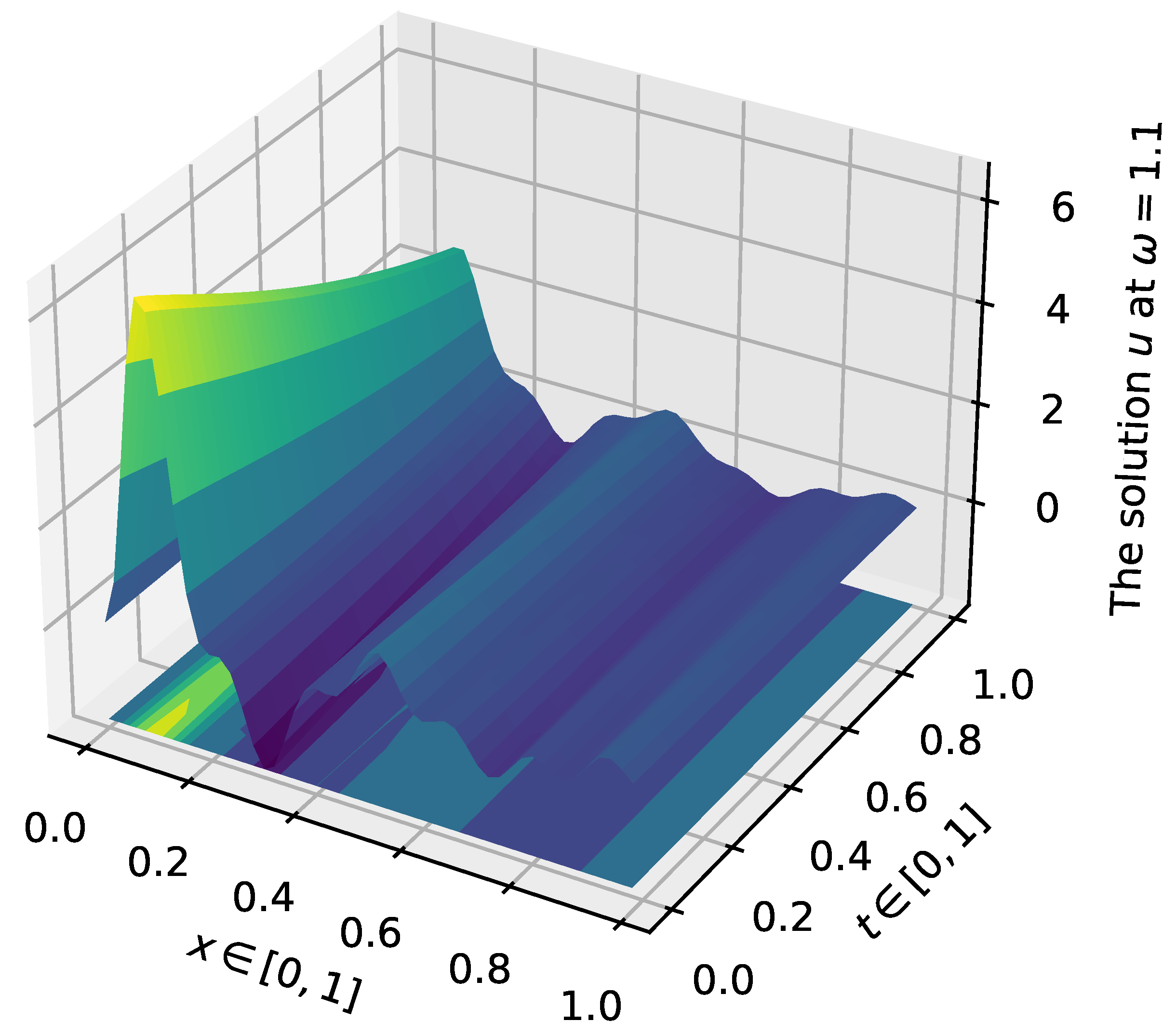
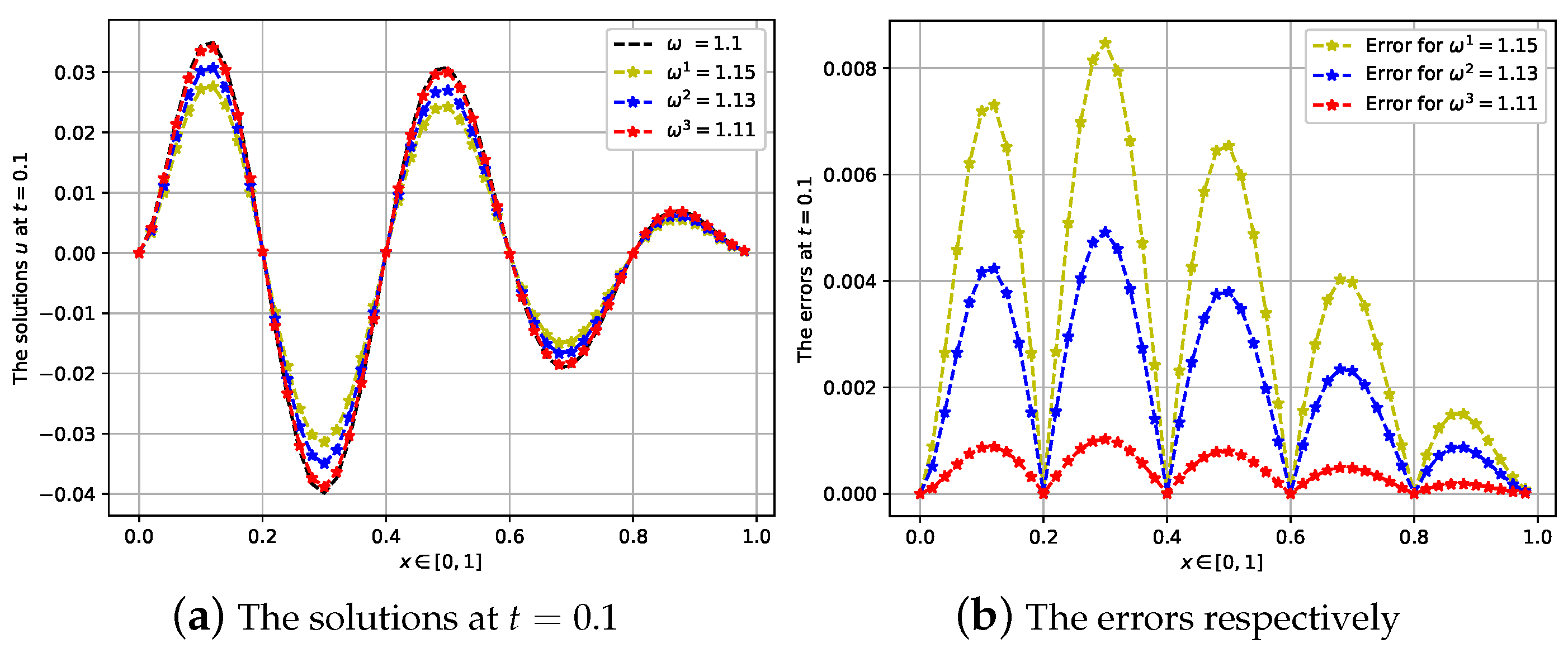
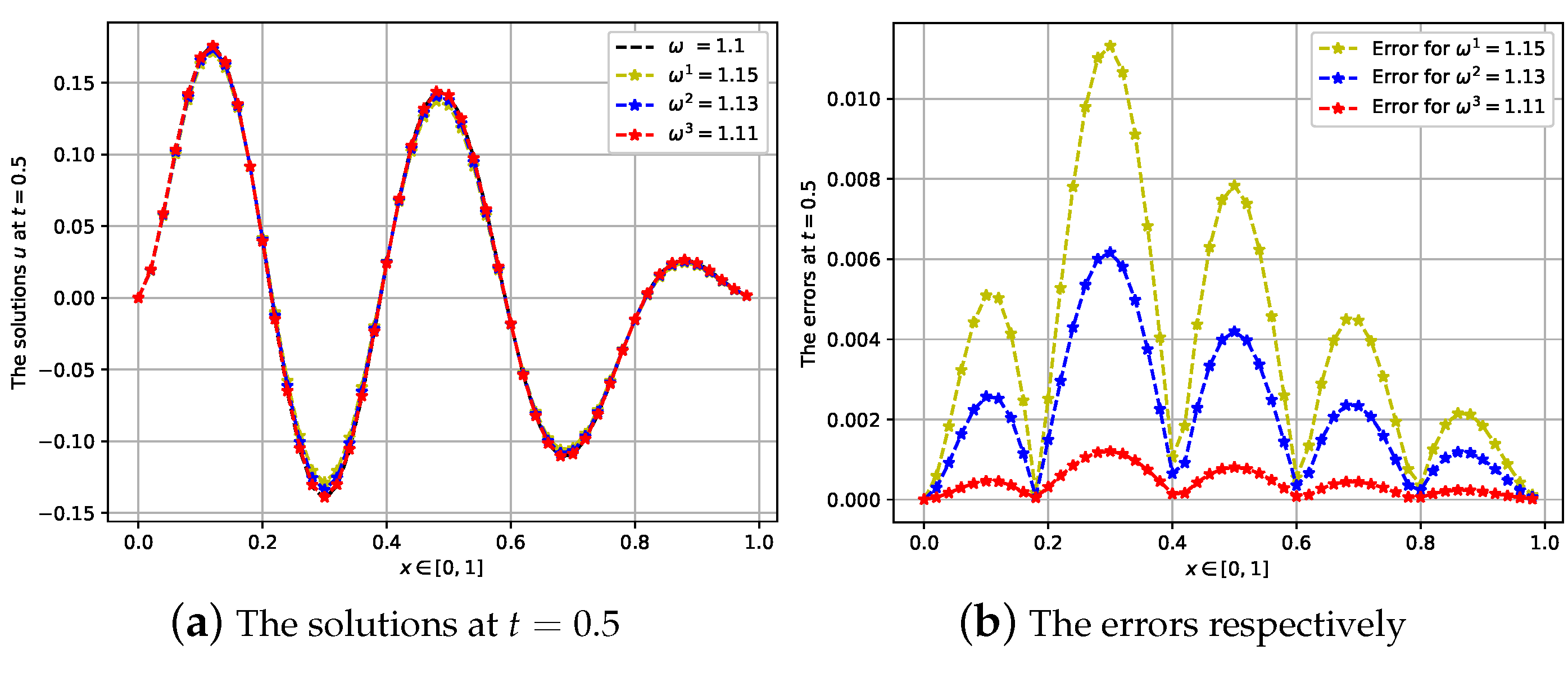
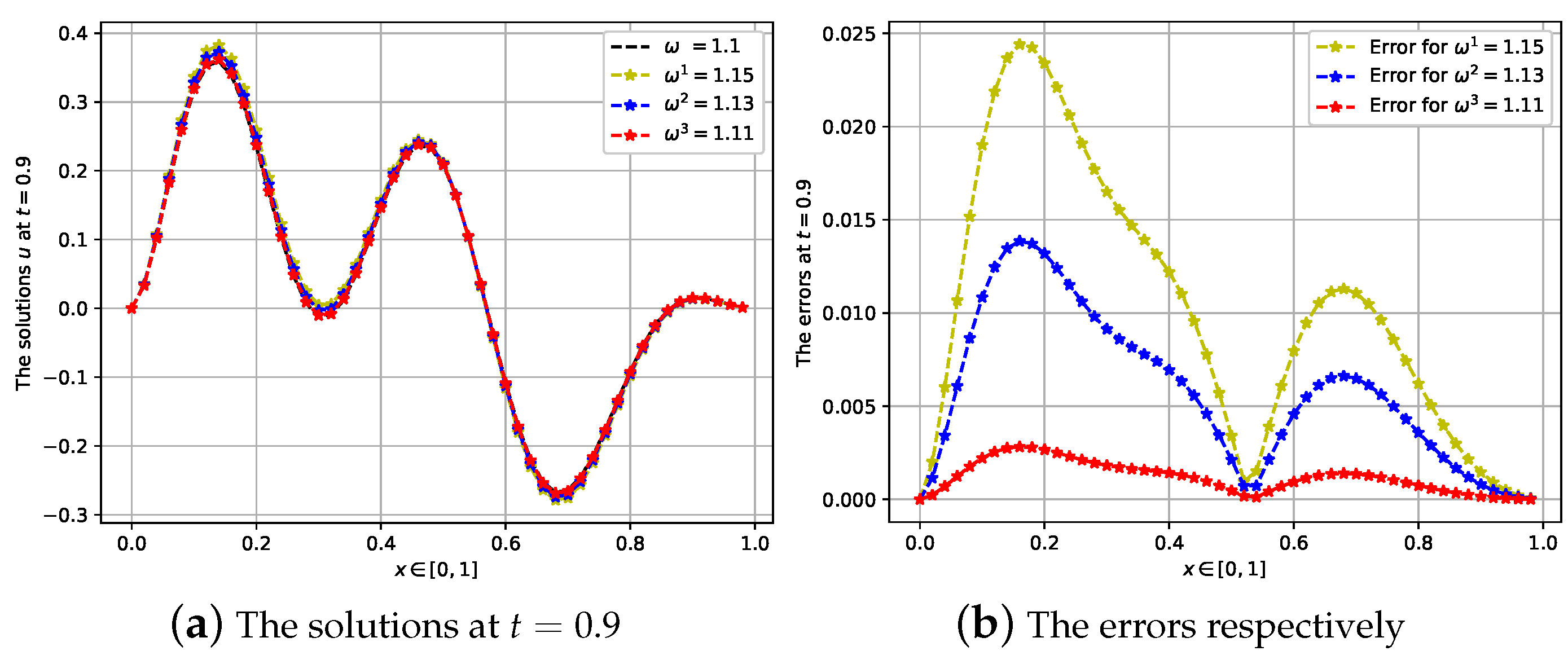
4. Numerical Experiments

In this section, we employ our proposed numerical scheme for the continuity fractional order for the pseudo-parabolic equation with the fractional Caputo derivative. For more detail, we present some examples to illustrate the property which are shown in Theorem 1. It means that the solution $u_{{\omega }^{\prime }}$ (the solution u with order ${\omega }^{\prime }$) converge on $u_{\omega }$ (the solution u with order ω) when ${\omega }^{\prime }$ tends to ω, where ω is the fractional order. To do this, firstly, we use finite difference to discrete the spatial and time variable on the domain $(x,t)\in [0,1]\times [0,1]$ as follows

$${\mathbb{D}}_x:=\left\{x_p={\displaystyle \frac{p-1}{N_x}},p=\overline{1,N_x+1}\right\},{\mathbb{D}}_t:=\left\{t_q={\displaystyle \frac{q-1}{N_t}},q=\overline{1,N_t+1}\right\},$$

where $N_x$ and $N_t$ are given positive constants.

Secondly, in calculations with Python software, we use some numerical approximation methods as follows.

We use the approximation of the Mittag-Leffler function $E_{\omega ,\varphi }$ as follows

$$\begin{array}{c}\hfill E_{\omega ,\varphi }\left(z\right):=\mathtt{ml}(z,\omega ,\varphi ),\end{array}$$

and we evaluate the function $\mathsf{\Gamma }(·)$ by $\mathtt{gamma}(·)$ function which defined in the Matplotlib library.

The integral approximation method by sum Rieamann. This approach can be used to find a numerical approximation for a definite integral

$${\int }_{z_1}^{z_2}f\left(z\right)dz\approx \sum _{m=0}^{M}f\left(z_1+m{\displaystyle \frac{z_2-z_1}{M}}\right){\displaystyle \frac{z_2-z_1}{M}},$$

where M is large enough positive number.

Next, by taking the operator $\mathcal{R}=-\Delta$. Then we have an orthonormal eigenbasis in $L^2(0,1)$ is

$$\begin{array}{c}\hfill {\psi }_n=\sqrt{2}sin\left(n\pi x\right),\end{array}$$

(44)

and the respective eigenvalues as follows

$$0<{\lambda }_1\le {\lambda }_2\le {\lambda }_3\le ...⟶\infty ,\mathrm{where}{\lambda }_n=n^2{\pi }^2,\mathrm{for}n\in {\mathbb{Z}}^{+}.$$

By choosing $T=1$ and $\kappa =1$, we focus on the following time fractional diffusion equation

$$\begin{array}{c}\hfill {\partial }_t^{\omega }\left(u(x,t)-u_{xx}(x,t)\right)-u_{xx}(x,t)=\mathcal{G}((x,t,u(x,t)),(x,t)\in (0,1)\times (0,1],\end{array}$$

(45)

subject to the initial conditions as follows

$$\begin{array}{c}\hfill u(x,t){|}_{t=0}=g_0\left(x\right)\mathrm{and}{u}_t(x,t){|}_{t=0}=0,x\in (0,1),\end{array}$$

(46)

and the Dirichlet boundary condition as follows

$$\begin{array}{c}\hfill u(x,t){|}_{x=0}=u(x,t){|}_{x=1}=0,t\in (0,1],\end{array}$$

(47)

Base on the solution (21), we can rewrite it in form truncation according to $\mathcal{N}$ which is a parameter truncated as follows

$$\begin{array}{cc}\hfill u(x,t)& {\displaystyle =\sum _{n=1}^{\mathcal{N}}{E}_{\omega ,1}\left({\displaystyle \frac{-n^2{\pi }^2{t}^{\alpha }}{1+n^2{\pi }^2}}\right){\int }_0^1{g}_0\left(\tau \right){\psi }_n\left(\tau \right)d\tau {\psi }_n\left(x\right)}\hfill \\ \hfill & +\sum _{n=1}^{\mathcal{N}}\frac{1}{1+n^2{\pi }^2}\left[{\int }_0^t{(t-s)}^{\omega }{E}_{\omega ,\omega }\left({\displaystyle \frac{-{(t-s)}^{\omega -1}{n}^2{\pi }^2}{1+n^2{\pi }^2}}\right){\mathcal{G}}_n\left(u_n\left(s\right)\right)\mathrm{d}s\right]{\psi }_n\left(x\right),\hfill \end{array}$$

(48)

where ${\displaystyle {\mathcal{G}}_n\left(u\left(s\right)\right):=\mathcal{G}(u(·,s),·,s)=〈\mathcal{G}(u(·,s),·,s),{\psi }_n(·)〉={\int }_0^1\mathcal{G}(u(\tau ,s),\tau ,s){\psi }_n\left(\tau \right)\mathrm{d}\tau }$.

On the domain $[0,1]\times [0,10]$, we have a performance below

$$\begin{array}{cc}\hfill u(x_p,t_q)& =2\left[\begin{array}{ccccc}{\tilde{u}}_1\left(t_q\right)& {\tilde{u}}_2\left(t_q\right)& {\tilde{u}}_3\left(t_q\right)& \cdots & {\tilde{u}}_{\mathcal{N}}\left(t_q\right)\end{array}\right]\hfill \\ \hfill & \times {\left[\begin{array}{ccccc}sin\left(\pi x_p\right)& sin\left(2\pi x_p\right)& sin\left(3\pi x_p\right)& \cdots & sin\left(\mathcal{N}\pi x_p\right)\end{array}\right]}^{\mathrm{T}},\hfill \end{array}$$

(49)

where ${\left[A\right]}^{\mathrm{T}}$ is the transposition matrix of the matrix $\left[A\right]$ and

$$\begin{array}{cc}\hfill {\tilde{u}}_1\left(t_q\right)& {\displaystyle =E_{\omega ,1}\left({\displaystyle \frac{-n^2{\pi }^2{t}_p^{\alpha }}{1+n^2{\pi }^2}}\right){\int }_0^1{g}_0\left(\tau \right){\psi }_n\left(\tau \right)d\tau }\hfill \\ \hfill & {\displaystyle +\frac{1}{1+n^2{\pi }^2}{\int }_0^{t_p}{(t_p-s)}^{\omega }{E}_{\omega ,\omega }\left({\displaystyle \frac{-{(t_p-s)}^{\omega -1}{n}^2{\pi }^2}{1+n^2{\pi }^2}}\right){\int }_0^1\mathcal{G}(u(\tau ,s),\tau ,s){\psi }_n\left(\tau \right)\mathrm{d}\tau \mathrm{d}s.}\hfill \end{array}$$

(50)

Then the solution (49) can be written in the matrix form ${\left[u_{pq}\right]}_{(N_x+1)\times (N_t+1)}$, where the representative element $u_{pq}$ of this matrix is $u(x_p,t_q)$.

Finally, by fixing t, we have the relative error estimation (${\mathcal{REE}}_{\omega }^{{\omega }^i}$) and percent error estimation (${\mathcal{PEE}}_{\omega }^{{\omega }^i}$) between the solutions $u_{\omega }$ and $u_{{\omega }^{\prime }}$ as follows

$$\begin{array}{cc}\hfill & {\mathcal{REE}}_{\omega }^{{\omega }^i}\left(t\right)=\sum _{p=1}^{N_x+1}|u_{{\omega }^i}(x_p,t)-u_{\omega }(x_p,t)|,\mathrm{for}\mathrm{some}\mathrm{cases}i=1,2,3.\hfill \end{array}$$

(51)

$$\begin{array}{cc}\hfill & {\mathcal{PEE}}_{\omega }^{{\omega }^i}\left(t\right)={\mathcal{REE}}_{\omega }^{{\omega }^i}\left(t\right)/{\displaystyle \sum _{p=1}^{N_x+1}\left|u_{\omega }(x_p,t)\right|}\times 100.\hfill \end{array}$$

(52)

Let get started, we consider $(x,t)$ on the domain $[0,1]\times [0,1]$ with the functions are given by

$$\begin{array}{cc}\hfill & g_0\left(x\right)=\sqrt{2}sin\left(2\pi x\right),\hfill \end{array}$$

(53)

$$\begin{array}{cc}\hfill & \mathcal{G}(u,x,t)=u^2-{\displaystyle \frac{4{\pi }^2\sqrt{2}}{t^2+1}}sin\left(2\pi x\right)+{\displaystyle \frac{cos\left(4\pi x\right)-1}{{(t^2+1)}^2}}.\hfill \end{array}$$

(54)

In the following subsection, by choosing $N_x=N_t=50$ and $\mathcal{N}=10$, we present the result of the numerical implementations for the problem (45) with the conditions (53) and (54) in some cases as follows.

4.1. First Case: The Fractional Order Is $\omega =1.1$

In this case, we consider the asymptotic behaviour of the solutions for some values of $\omega =1.1$ and ${\omega }^i\in \{1.15,1.13,1.11\}$.

The numerical result is shown that the performance of the proposed method is acceptable. Indeed, the convergent estimate between the solutions for the fractional orders ω and ${\omega }^i$ at $t\in \{0.1,0.5,0.9\}$ is shown in

Table 1. The relative error and percent error estimations for $\omega =1.1$.

Fractional Order	$\mathit{t}=0.1$		$\mathit{t}=0.5$		$\mathit{t}=0.9$
	${\mathcal{REE}}_{\mathit{\omega }}^{{\mathit{\omega }}^{\mathbf{i}}}$	${\mathcal{PEE}}_{\mathit{\omega }}^{{\mathit{\omega }}^{\mathbf{i}}}$	${\mathcal{REE}}_{\mathit{\omega }}^{{\mathit{\omega }}^{\mathbf{i}}}$	${\mathcal{PEE}}_{\mathit{\omega }}^{{\mathit{\omega }}^{\mathbf{i}}}$	${\mathcal{REE}}_{\mathit{\omega }}^{{\mathit{\omega }}^{\mathbf{i}}}$	${\mathcal{PEE}}_{\mathit{\omega }}^{{\mathit{\omega }}^{\mathbf{i}}}$
${\omega }^1=1.15$	0.17060940	21.16%	0.19486871	5.23%	0.50700111	7.41%
${\omega }^2=1.13$	0.09891093	12.26%	0.10425578	2.80%	0.28847739	4.22%
${\omega }^3=1.11$	0.02063175	2.55%	0.02002432	0.53%	0.05891203	0.86%

,

Table 2. The relative error and percent error estimations for $\omega =1.5$.

Fractional Order	$\mathit{t}=0.1$		$\mathit{t}=0.5$		$\mathit{t}=0.9$
	${\mathcal{REE}}_{\mathit{\omega }}^{{\mathit{\omega }}^{\mathbf{i}}}$	${\mathcal{PEE}}_{\mathit{\omega }}^{{\mathit{\omega }}^{\mathbf{i}}}$	${\mathcal{REE}}_{\mathit{\omega }}^{{\mathit{\omega }}^{\mathbf{i}}}$	${\mathcal{PEE}}_{\mathit{\omega }}^{{\mathit{\omega }}^{\mathbf{i}}}$	${\mathcal{REE}}_{\mathit{\omega }}^{{\mathit{\omega }}^{\mathbf{i}}}$	${\mathcal{PEE}}_{\mathit{\omega }}^{{\mathit{\omega }}^{\mathbf{i}}}$
${\omega }^1=1.55$	0.06218532	23.58%	0.25924582	9.55%	0.20731152	2.48%
${\omega }^2=1.53$	0.03645685	13.82%	0.14441751	5.32%	0.11992968	1.43%
${\omega }^3=1.51$	0.00769853	2.92%	0.02891043	1.06%	0.02491671	0.29%

and

Table 3. The relative error and percent error estimations for $\omega =1.9$.

Fractional Order	$\mathit{t}=0.1$		$\mathit{t}=0.5$		$\mathit{t}=0.9$
	${\mathcal{REE}}_{\mathit{\omega }}^{{\mathit{\omega }}^{\mathbf{i}}}$	${\mathcal{PEE}}_{\mathit{\omega }}^{{\mathit{\omega }}^{\mathbf{i}}}$	${\mathcal{REE}}_{\mathit{\omega }}^{{\mathit{\omega }}^{\mathbf{i}}}$	${\mathcal{PEE}}_{\mathit{\omega }}^{{\mathit{\omega }}^{\mathbf{i}}}$	${\mathcal{REE}}_{\mathit{\omega }}^{{\mathit{\omega }}^{\mathbf{i}}}$	${\mathcal{PEE}}_{\mathit{\omega }}^{{\mathit{\omega }}^{\mathbf{i}}}$
${\omega }^1=1.95$	0.01925768	24.99%	0.20146470	12.17%	0.31121755	3.82%
${\omega }^2=1.93$	0.01134916	14.72%	0.11418913	6.89%	0.16942761	2.08%
${\omega }^3=1.91$	0.00241016	3.12%	0.02328528	1.40%	0.03311517	0.40%

.

In addition, we present the graphs of the solutions and corresponding errors in Figures. To facilitate comparison, we consider three cases of the fractional order such as $\omega \in \{1.1,1.5,1.9\}$. We also show the 3D-graph of the solutions u on the domain $(x,t)\in [0,1]\times [0,1]$. For detail, the first case $\omega =1.1$ is shown in Figure 1, Figure 2, Figure 3 and Figure 4. The second case $\omega =1.5$ is shown in Figure 5, Figure 6, Figure 7 and Figure 8. And the final case, $\omega =1.9$ is shown in Figure 9, Figure 10, Figure 11 and Figure 12.

From the observations on these tables and figures, it concludes that the smaller the error output between the solutions for the fractional orders ω and ${\omega }^i$ when the smaller in the fractional orders.

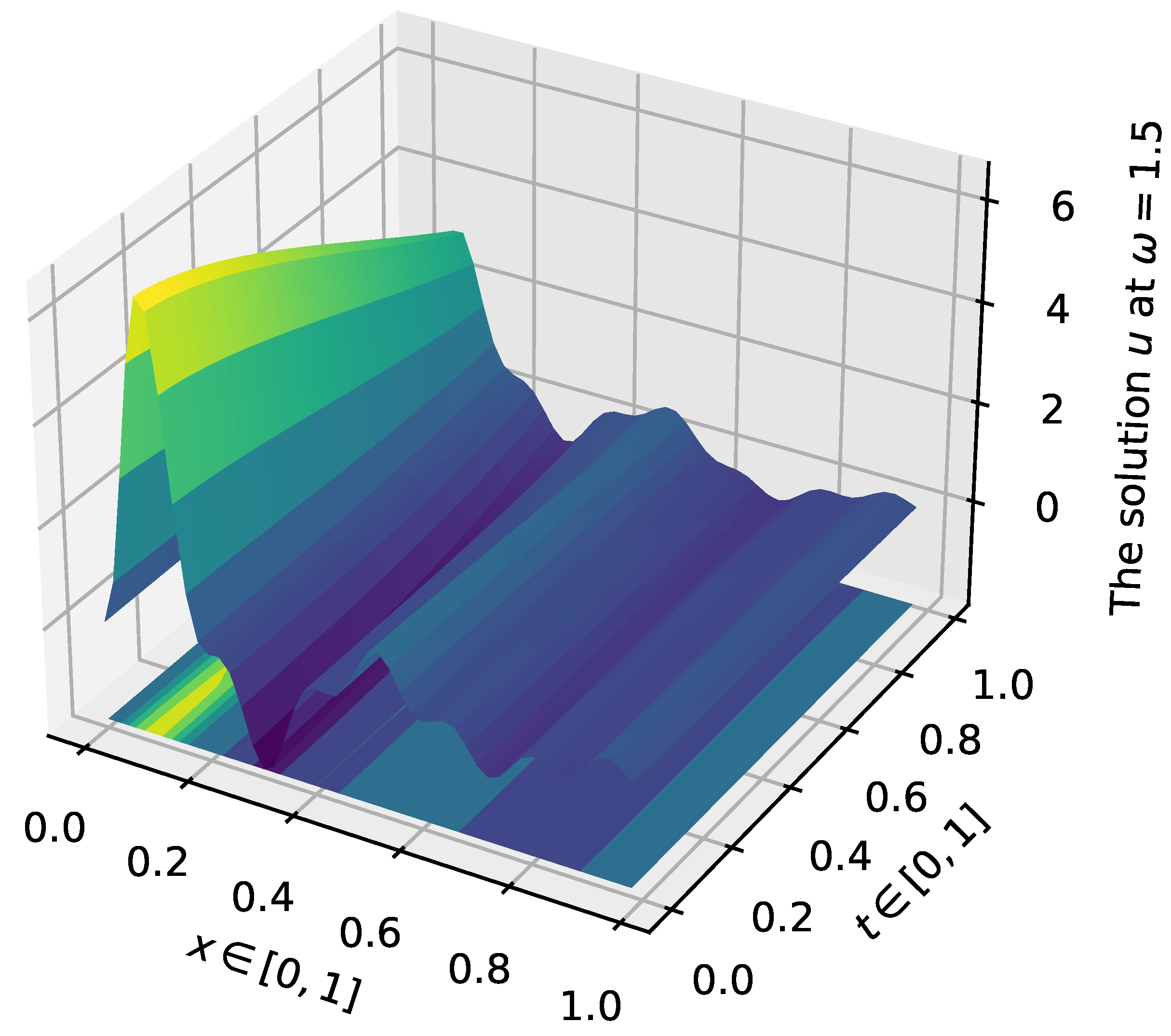
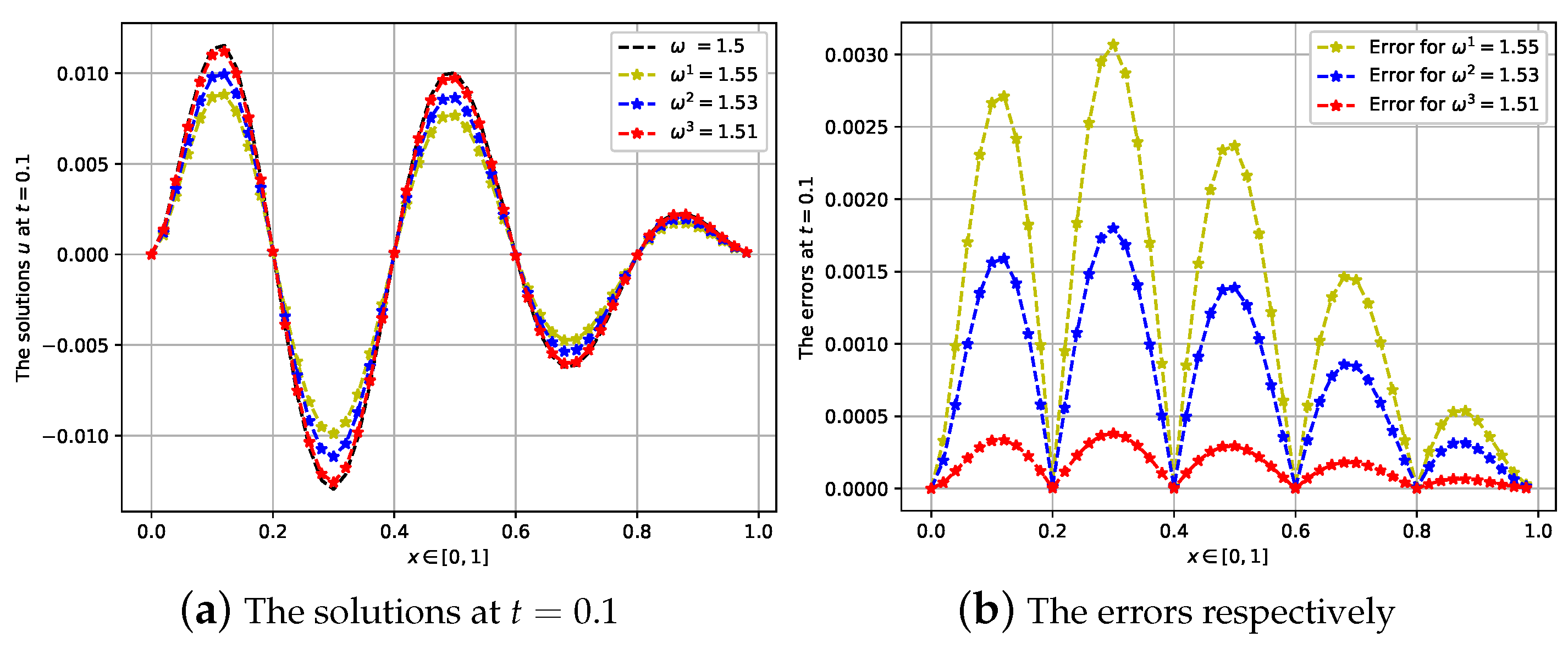
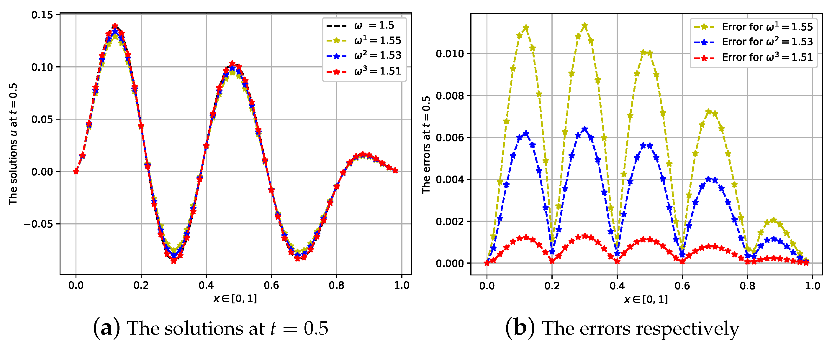
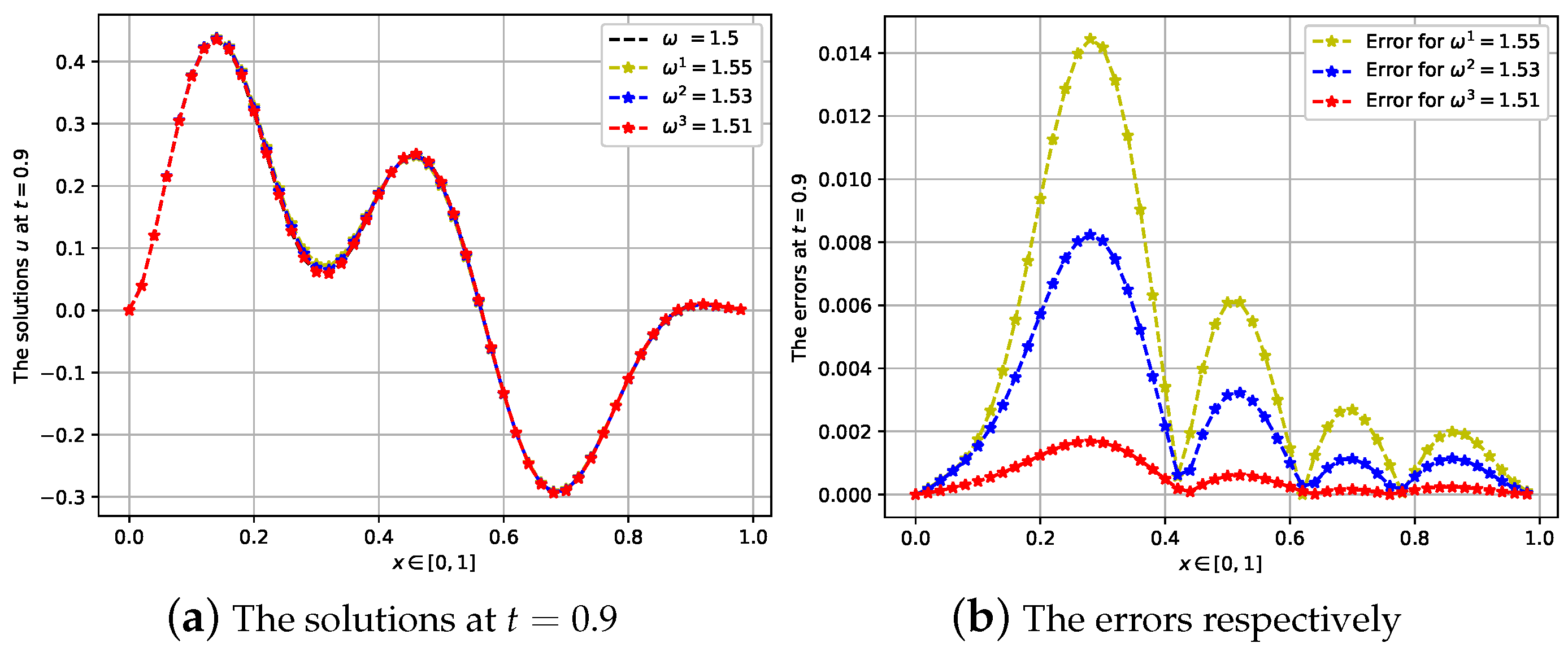
4.2. Second Case: The Fractional Order Is ω = 1.5

In this subsection, we consider the asymptotic behaviour of the solutions for some values of $\omega =1.5$ and ${\omega }^i\in \{1.55,1.53,1.51\}$.

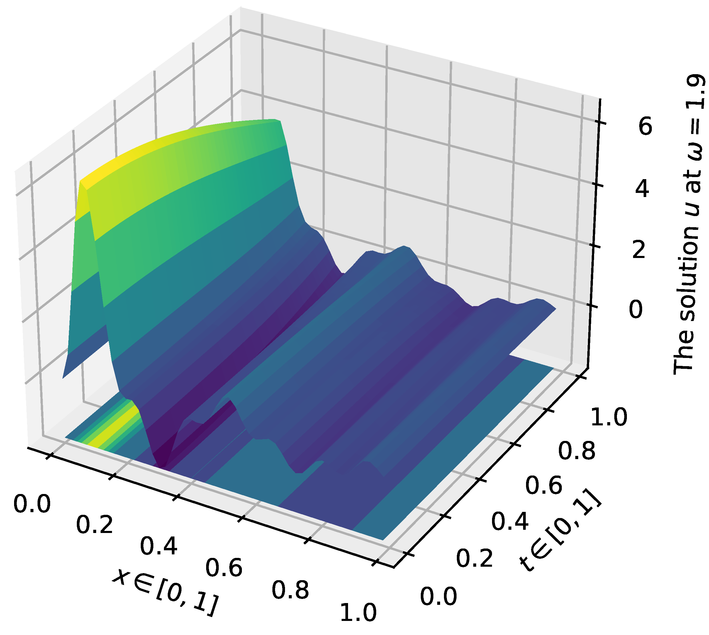
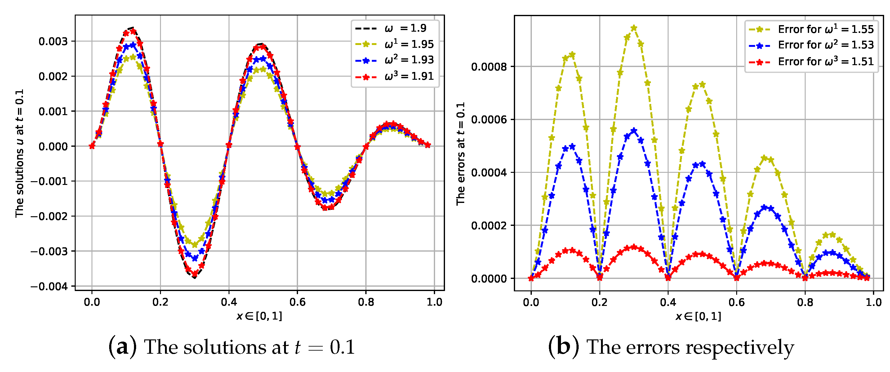
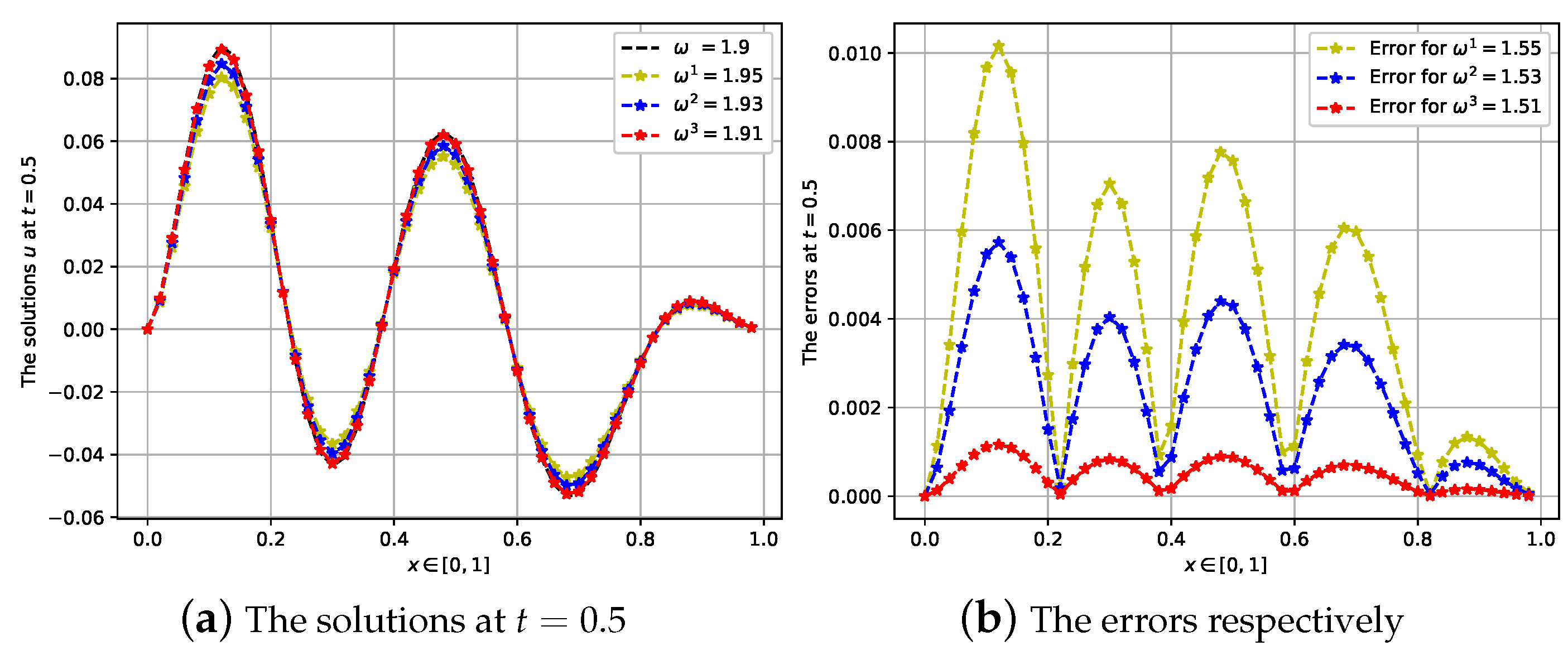
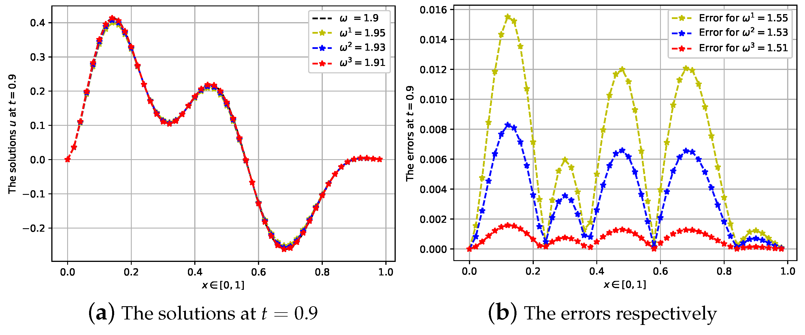
4.3. Third Case: The Fractional Order Is ω = 1.9

In final case, we consider the asymptotic behaviour of the solutions for some values of $\omega =1.9$ and ${\omega }^i\in \{1.95,1.93,1.91\}$.

References

1. Atangana, A.; Akgül, A.; Owolabi, K.M. Analysis of fractal fractional differential equations. Alex. Eng. J. 2020, 59, 1117–1134. [Google Scholar] [CrossRef]
2. Atangana, A.; Hammouch, Z. Fractional calculus with power law: The cradle of our ancestors. Eur. Phys. J. Plus 2019, 134, 429. [Google Scholar] [CrossRef]
3. Atangana, A.; Bonyah, E. Fractional stochastic modeling: New approach to capture more heterogeneity. Chaos Interdiscip. J. Nonlinear Sci. 2019, 29, 013118. [Google Scholar] [CrossRef] [PubMed]
4. Atangana, A.A.; Baleanu, D. New fractional derivatives with nonlocal and non-singular kernel: Theory and application to heat transfer model. Therm. Sci. 2016, 18. [Google Scholar] [CrossRef] [Green Version]
5. Atangana, A.; Goufo, E.F.D. Cauchy problems with fractal-fractional operators and applications to groundwater dynamics. Fractals 2020. [Google Scholar] [CrossRef]
6. Sun, H.G.; Zhang, Y.; Baleanu, D.; Chen, W.; Chen, Y.Q. A new collection of real world applications of fractional calculus in science and engineering. Commun. Nonlinear Sci. Numer. Simul. 2018, 64, 213–231. [Google Scholar] [CrossRef]
7. Podlubny, I. Fractional Differential Equations; Academic press: Cambridge, MA, USA, 1999. [Google Scholar]
8. Abro, K.A.; Atangana, A. Mathematical analysis of memristor through fractal -fractional differential operators: A numerical study. Math. Methods Appl. Sci. 2020, 43, 6378–6395. [Google Scholar] [CrossRef]
9. Tuan, N.H.; Baleanu, D.; Thach, T.N.; O’Regan, D.; Can, N.H. Final value problem for nonlinear time fractional reaction-diffusion equation with discrete data. J. Comput. Appl. Math. 2020, 376, 112883. [Google Scholar] [CrossRef]
10. Luc, N.H.; Huynh, L.N.; Baleanu, D.; Can, N.H. Identifying the space source term problem for a generalization of the fractional diffusion equation with hyper-Bessel operator. Adv. Differ. Equ. 2020, 261, 23. [Google Scholar] [CrossRef]
11. Sweilam, N.H.; Al-Mekhlafi, S.M.; Assiri, T.; Atangana, A. Optimal control for cancer treatment mathematical model using Atangana-Baleanu-Caputo fractional derivative. Adv. Differ. Equ. 2020, 334. [Google Scholar] [CrossRef]
12. Tuan, N.H.; Huynh, L.N.; Baleanu, D.; Can, N.H. On a Terminal Value Problem for a Generalization of the Fractional Diffusion Equation with Hyper-Bessel Operator. Math. Methods Appl. Sci. 2020, 43, 2858–2882. [Google Scholar] [CrossRef]
13. Kumar, S.; Atangana, A. A numerical study of the nonlinear fractional mathematical model of tumor cells in presence of chemotherapeutic treatment. Int. J. Biomath. 2020, 13, 2050021. [Google Scholar] [CrossRef]
14. Kiryakova, V. Generalized Fractional Calculus and Applications; CRC press: Boca Raton, FL, USA, 1993. [Google Scholar]
15. Ngoc, T.B.; Baleanu, D.; Duc, L.M.; Tuan, N.H. Regularity results for fractional diffusion equations involving fractional derivative with Mittag-Leffler kernel. Math. Methods Appl. Sci. 2020, 43, 7208–7226. [Google Scholar]
16. Ebaid, A.; Cattani, C.; Al Juhani, A.S.; El-Zahar, E.R. A novel exact solution for the fractional Ambartsumian equation. Adv. Differ. Equ. 2021, 2021, 88. [Google Scholar] [CrossRef]
17. Heydaria, M.H.; Avazzadehb, Z.; Cattani, C. Taylor’s series expansion method for nonlinear variable-order fractional 2D optimal control problems. Alex. Eng. J. 2020, 59, 4737–4743. [Google Scholar] [CrossRef]
18. Mohammad, M.; Cattani, C. A collocation method via the quasi-affine biorthogonal systems for solving weakly singular type of Volterra-Fredholm integral equations. Alex. Eng. J. 2020, 59, 2181–2191. [Google Scholar] [CrossRef]
19. Li, L.; Liu, G.J. A generalized definition of Caputo derivatives and its application to fractional ODEs. SIAM J. Math. Anal. 2018, 50, 2867–2900. [Google Scholar] [CrossRef] [Green Version]
20. Benjamin, T.B.; Bona, J.L.; Mahony, J.J. Model equations for long waves in nonlinear dispersive systems. Philos. Trans. R. Soc. 1972, 272, 47–78. [Google Scholar]
21. Ting, W.T. Certain non-steady flows of second-order fluids. Arch. Ration. Mech. Anal. 1963, 14, 1–26. [Google Scholar] [CrossRef]
22. Padron, V. Effect of aggregation on population recovery modeled by a forward-backward pseudo-parabolic equation. Trans. Am. Math. Soc. 2004, 356, 2739–2756. [Google Scholar] [CrossRef]
23. Huafei, D.; Yadong, S.; Xiaoxiao, Z. Global well-posedness for a fourth order pseudo-parabolic equation with memory and source terms. Disc. Contin. Dyn. Syst. Ser. B 2016, 21, 781–801. [Google Scholar]
24. Sun, F.; Liu, L.; Wu, Y. Global existence and finite time blow-up of solutions for the semi-linear pseudo-parabolic equation with a memory term. Appl. Anal. 2019, 98, 22. [Google Scholar] [CrossRef]
25. Ding, H.; Zhou, J. Global existence and blow-up for a mixed pseudo-parabolic p-Laplacian type equation with logarithmic nonlinearity. J. Math. Anal. Appl. 2019, 478, 393–420. [Google Scholar] [CrossRef]
26. Jin, L.; Li, L.; Fang, S. The global existence and time-decay for the solutions of the fractional pseudo-parabolic equation. Comput. Math. Appl. 2017, 73, 2221–2232. [Google Scholar] [CrossRef]
27. Afshari, H.; Kalantari, S.; Karapinar, E. Solution of fractional differential equations via coupled fixed point. Electron. J. Differ. Equ. 2015, 2015, 1–12. [Google Scholar]
28. Karapinar, E.; Fulga, A.; Rashid, M.; Shahid, L.; Aydi, H. Large Contractions on Quasi-Metric Spaces with an Application to Nonlinear Fractional Differential-Equations. Mathematics 2019, 7, 444. [Google Scholar] [CrossRef] [Green Version]
29. Karapinar, E.; Abdeljawad, T.; Jarad, F. Applying new fixed point theorems on fractional and ordinary differential equations. Adv. Differ. Equ. 2019, 2019, 421. [Google Scholar] [CrossRef] [Green Version]
30. Abdeljawad, A.; Agarwal, R.P.; Karapinar, E.; Kumari, P.S. Solutions of he Nonlinear Integral Equation and Fractional Differential Equation Using the Technique of a Fixed Point with a Numerical Experiment in Extended b-Metric Space. Symmetry 2019, 11, 686. [Google Scholar] [CrossRef] [Green Version]
31. Zhu, X.; Li, F.; Li, Y. Global solutions and blow up solutions to a class of pseudo-parabolic equations with nonlocal term. Appl. Math. Comput. 2018, 329, 38–51. [Google Scholar] [CrossRef]
32. Cao, Y.; Yin, J.; Wang, C. Cauchy problems of semilinear pseudo-parabolic equations. J. Differ. Equ. 2009, 246, 4568–4590. [Google Scholar] [CrossRef] [Green Version]
33. Cao, Y.; Liu, C. Initial boundary value problem for a mixed pseudo- parabolic p-Laplacian type equation with logarithmic nonlinearity. Electron. J. Differ. Equ. 2018, 2018, 1–19. [Google Scholar]
34. He, Y.; Gao, H.; Wang, H. Blow-up and decay for a class of pseudo-parabolic p-Laplacian equation with logarithmic nonlinearity. Comput. Math. Appl. 2018, 75, 459–469. [Google Scholar] [CrossRef]
35. Lu, Y.; Fei, L. Bounds for blow-up time in a semilinear pseudo-parabolic equation with nonlocal source. J. Inequalities Appl. 2016, 2016, 229. [Google Scholar] [CrossRef] [Green Version]
36. Sousa, C.V.J.; de Oliveira, C.E. Fractional order pseudo-parabolic partial differential equation: Ulam-Hyers stability. Bull. Braz. Math. Soc. 2019, 50, 481–496. [Google Scholar] [CrossRef] [Green Version]
37. Beshtokov, M.K. To boundary-value problems for degenerating pseudo-parabolic equations with Gerasimov-Caputo fractional derivative. Izv. Vyssh. Uchebn. Zaved. Mat. 2018, 10, 3–16. [Google Scholar]
38. Beshtokov, M.K. Boundary-value problems for loaded pseudo-parabolic equations of fractional order and difference methods of their solving. Russ. Math. 2019, 63, 1–10. [Google Scholar] [CrossRef]
39. Beshtokov, M.K. Boundary value problems for a pseudoparabolic equation with the Caputo fractional derivative. Differ. Equ. 2019, 55, 884–893. [Google Scholar] [CrossRef]
40. Dang, D.T.; Nane, E.; Nguyen, D.M.; Tuan, N.H. Continuity of Solutions of a Class of Fractional Equations. Potential Anal. 2018, 49, 423–478. [Google Scholar] [CrossRef] [Green Version]
41. Tuan, N.H.; O’Regan, D.; Ngoc, T.B. Continuity with respect to fractional order of the time fractional diffusion-wave equation. Evol. Equ. Control Theory 2020, 9, 773. [Google Scholar] [CrossRef] [Green Version]
42. Samko, S.G.; Kilbas, A.A.; Marichev, O.I. Fractional Integrals and Derivatives, Theory and Applications; Gordon and Breach Science: Naukai Tekhnika, Minsk, 1987. [Google Scholar]
43. Diethelm, K. The Analysis of Fractional Differential Equations; Springer: Berlin/Heidelberg, Germany, 2010. [Google Scholar]
44. Wei, T.; Zhang, Y. The backward problem for a time-fractional diffusion-wave equation in a bounded domain. Comput. Math. Appl. 2018, 75, 3632–3648. [Google Scholar] [CrossRef]
45. Sakamoto, K.; Yamamoto, M. Initial value/boundary value problems for fractional diffusion-wave equations and applications to some inverse problems. J. Math. Anal. Appl. 2011, 382, 426–447. [Google Scholar] [CrossRef] [Green Version]
46. Kato, T. Perturbation Theory for Linear Operators; Springer: Berlin/Heidelberg, Germany, 1995. [Google Scholar]
47. Kilbas, A.A.; Srivastava, H.M.; Trujillo, J.J. Theory and Applications of Fractional Differential Equations; Elsevier Science B.V.: Amsterdam, The Netherlands, 2006. [Google Scholar]
Figure 1. The 3-dimensional graph of solution u on the domain ( x , t ) [ 0 , 1 ] × [ 0 , 1 ] for ω = 1.1 .
Fractalfract 05 00041 g001
Figure 2. The solution u for ω = 1.1 , ω i { 1.15 , 1.13 , 1.11 } at t = 0.1 and the respective error.
Fractalfract 05 00041 g002
Figure 3. The solution u for ω = 1.1 , ω i { 1.15 , 1.13 , 1.11 } at t = 0.5 and the respective error.
Fractalfract 05 00041 g003
Figure 4. The solution u for ω = 1.1 , ω i { 1.15 , 1.13 , 1.11 } at t = 0.9 and the respective error.
Fractalfract 05 00041 g004
Figure 5. The 3-dimensional graph of solution u on the domain ( x , t ) [ 0 , 1 ] × [ 0 , 1 ] for ω = 1.5 .
Fractalfract 05 00041 g005
Figure 6. The solution u for ω = 1.5 , ω i { 1.55 , 1.53 , 1.51 } at t = 0.1 and the respective error.
Fractalfract 05 00041 g006
Figure 7. The solution u for ω = 1.5 , ω i { 1.55 , 1.53 , 1.51 } at t = 0.5 and the respective error.
Fractalfract 05 00041 g007
Figure 8. The solution u for ω = 1.5 , ω i { 1.55 , 1.53 , 1.51 } at t = 0.9 and the respective error.
Fractalfract 05 00041 g008
Figure 9. The 3-dimensional graph of solution u on the domain ( x , t ) [ 0 , 1 ] × [ 0 , 1 ] for ω = 1.9 .
Fractalfract 05 00041 g009
Figure 10. The solution u for ω = 1.9 , ω i { 1.95 , 1.93 , 1.91 } at t = 0.1 and the respective error.
Fractalfract 05 00041 g010
Figure 11. The solution u for ω = 1.9 , ω i { 1.95 , 1.93 , 1.91 } at t = 0.5 and the respective error.
Fractalfract 05 00041 g011
Figure 12. The solution u for ω = 1.9 , ω i { 1.95 , 1.93 , 1.91 } at t = 0.9 and the respective error.
Fractalfract 05 00041 g012