Article

Analysis of Fractional Order Chaotic Financial Model with Minimum Interest Rate Impact

1
Department of Mathematics and Statistics, University of Lahore, Lahore 54590, Pakistan
2
Art and Science Faculty, Department of Mathematics, Siirt University, Siirt 56100, Turkey
3
Department of Mathematics, Cankaya University, Ankara 06530, Turkey
4
Institute of Space Sciences, R76900 Magurele-Bucharest, Romania
5
Department of Medical Research, China Medical University, Taichung 40402, Taiwan
*
Author to whom correspondence should be addressed.
Fractal Fract. 2020, 4(3), 43; https://doi.org/10.3390/fractalfract4030043
Submission received: 19 July 2020 / Revised: 10 August 2020 / Accepted: 14 August 2020 / Published: 21 August 2020

Abstract

:
The main objective of this paper is to construct and test fractional order derivatives for the management and simulation of a fractional order disorderly finance system. In the developed system, we add the critical minimum interest rate d parameter in order to develop a new stable financial model. The new emerging paradigm increases the demand for innovation, which is the gateway to the knowledge economy. The derivatives are characterized in the Caputo fractional order derivative and Atangana-Baleanu derivative. We prove the existence and uniqueness of the solutions with fixed point theorem and an iterative scheme. The interest rate begins to rise according to initial conditions as investment demand and price exponent begin to fall, which shows the financial system’s actual macroeconomic behavior. Specifically component of its application to the large scale and smaller scale forms, just as the utilization of specific strategies and instruments such fractal stochastic procedures and expectation.

1. Introduction

Different parts of the financial sector are investigated through mathematical models, this article is helpful in discussing advantages and drawbacks of mathematical models in the financial associations. Different solutions for improving mathematical models and obstructions in the application zone is also discussed. Mathematical modeling is the technique in which sensible and similar numerical expressions from vertical frameworks are made which is used in translating different issues including drawing systematic ideas. These systematic ideas are used in formulating strategy by choosing information and understanding problem [1]. Mathematical models help in different fields of science such as sociology and engineering. Mathematics have an important place in the field of finance. In the field of finance, account related theory on assessment of exercises on the money related administrators [2]. Different parts of financial market types and different scientific and numerical systems are drawn by using mathematical models [3].
Different types of genuine certified systems are derived through the device of fractional calculus [4]. We establish some writing with the help of the research work and construct the hypothesis of fractional calculus and exhibiting several utilizations. The recently presented Caputo Fabrizio fractional derivative is used to examine the partial model of an adjusted Kawahara condition by Kumar et al. [5]. The Atangana-Baleanu partial administrator is used to formulate fragmentary augmentation of a regularized long wave condition [6]. Arrangement of the fragmentary control issues including a Mittag–Leffler non-specific piece is proposed by Baleanu et al. [7]. In another work, the development of fractional analysis has been given in [8]. Fractional calculus is used by the scientist named Jajarmi for separating a hyperchaotic financial system [9]. The fractional calculus operatives including different functions have been derived effectively for mathematical modeling of various complex issues in changed areas of science and engineering, for example, liquid elements, plasma material science, astronomy, picture handling, stochastic dynamical framework, and controlled atomic combination [1,10,11,12]. Recently, Caputo and Fabrizio [13] derived another fractional derivative for some engineering and thermo dynamical systems, and this new derivation is better than the old style of Caputo derivative. Another fractional derivative for observing the possibility of Fisher’s response dispersion condition is derived by Atangana [14]. In this article [15], by using these two approaches, we have defined a new contraction in one of the most extended abstract spaces known. In [16], we have demonstrated a novel approximate-analytical solution method, which is called the Laplace homotopy analysis method (LHAM) using the Caputo–Fabrizio fractional derivative operator. We investigated in [17] existence and uniqueness conditions of solutions of a nonlinear differential equation containing the Caputo–Fabrizio operator in Banach spaces. A solution method is coupled with a kind of integral transformation, namely the Elzaki transform, and apply it to two different nonlinear regularized long wave equations in [18]. In [19], time-fractional partial differential equations (FPDEs) involving singular and non-singular kernel are considered. For more details, see [20,21,22].
In this paper, we need to use fractional parameters using the Caputo and ABC derivatives method with fractional derivatives to build the model of complex nonlinear differential equations. Complex financial system models of complex actions provide a new perspective as a result of patterns and actual behavior of the financial system’s internal structure.

2. Preliminaries

The fractional derivative of Liouville Caputo [13,23] is presented as
t 0 C D t κ { g ( t ) } = 1 Γ ( 1 κ ) t 0 t d d t g ( ψ ) ( t ψ ) κ d ψ ,
where Γ ( . ) refers to the function of Gamma. Laplace transform of the above derivative is obtained as [23,24]:
L { 0 C D t κ { g ( t ) } } ( s ) = S κ G ( S ) k = 0 m 1 S κ k 1 g ( k ) ( 0 ) .
Recently, Atangana and Baleanu proposed a fractional derivative with the Mittag–Leffler function as the kernel of differentiation. This kernel is non-singular and nonlocal and preserves the benefits of the above Liouville–Caputo derivative. The Atangana–Baleanu derivative has been defined as [25]:
t 0 A B C D t κ { g ( t ) } = Z ( κ ) 1 κ t 0 t d d t g ( ψ ) E κ [ κ ( t ψ ) κ 1 κ ] d ψ , n 1 < κ ( t ) n ,
where κ ϵ , Z ( κ ) refers to the Z ( 0 ) = Z ( 1 ) = 1 and E κ ( . ) refers to the equation Mittag–Leffler. Equation (3) Laplace is defined as follows:
L { 0 A B C D t κ { g ( t ) } } ( s ) = Z ( κ ) 1 κ L [ κ t d d t g ( ψ ) E κ [ κ ( t ψ ) κ 1 κ ] d ψ ] ( s ) = Z ( κ ) 1 κ s κ L [ g ( t ) ] ( s ) s κ 1 g ( 0 ) s κ + κ 1 κ
The fractional integral associated with the Atangana–Baleanu derivative with non-local kernel is defined as
t 0 A B D t κ { g ( t ) } = 1 κ Z ( κ ) g ( t ) + κ Z ( κ ) Γ ( κ ) t 0 t g ( ψ ) ( t ψ ) κ 1 d ψ ,
When κ is equivalent to zero, the initial function will be retrieved. κ = 1 will be retrieved from the classical ordinary integral.

3. Liouville–Caputo Sense

The strategy is an experimental system dependent on the blend of homotopy analysis technique and Laplace’s transformation with polynomial homotopy [23,26]. The primary steps of this strategy are characterized as follows:
Step 1. We should take a look at the following condition:
D t κ { g ( h , t ) } + Ξ [ h ] g ( h , t ) + [ h ] g ( h , t ) = η ( h , t ) , t > 0 , h ϵ , 0 < κ 1 ,
where Ξ [ h ] is a bounded linear operator in h. While the nonlinear operator [ h ] in h is Lipschitz continuous and satisfying | ( g ) ( ϕ ) | θ | g ϕ | , where θ > 0 and η ( h , t ) is a continuous function. The boundary and initial conditions can be treated in a similar way.
Step 2. Applying the methodology proposed in [23,27], we get the following m-th order deformation equation:
g m ( h , t ) = ( X m + ) g m 1 ( 1 X m ) i = 0 j 1 t i g ( i 1 ) ( 0 ) + L 1 ( 1 s κ L ( Ξ m 1 [ h ] g m 1 ( h ) + k = 0 m 1 P k ( g 0 , g 1 , . . . . , g m ) Ψ ( h , t ) ) ) ,
where the Laplace transform is implemented in Caputo sense (1) and P k is the homotopy polynomial described by Odibat in [28].
Step 3. Regarding homotopy polynomials, the nonlinear term [ h ] g ( h , t ) is extended as
[ g ( h , t ) ] = ( k = 0 m 1 g m ( h , t ) ) = m = 0 P m g m
Step 4. Expanding the nonlinear term in (6) as a progression of polynomials for homotopy, we can compute the diverse g m ( h , t ) for m > 1 and Equation solutions (5) can be written as
g ( h , t ) = m = 0 g m ( h , t ) .
The classical form of the model first studied in [29] and we modify the model by adding d as critical minimum interest rate. By using this methodology, a Liouville–Caputo fractional order derivative was utilized to solve the using time-fractional funding model:
0 C D t κ x ( t ) = z ( t ) + x ( t ) y ( t ) a x ( t ) ,
0 C D t κ y ( t ) = 1 b y ( t ) x ( t ) x ( t ) ,
0 C D t κ z ( t ) = d x ( t ) c z ( t ) ,
where x, y, and z are the state variables representing interest rate, investment demand, and price index, respectively, and we add the critical minimum interest rate d parameter in [30]. The parameter a is for savings, b is to cost per investment and c is the elasticity of market demand, although the parameters are non-negative constants i.e., a = 3 , b = 0.1 and c = 1 .
From the above model (10)–(12), we use the parameter d to modify the model, where d represents critical minimum interest rate with initial conditions x ( 0 ) = n 1 = 0.1 , y ( 0 ) = n 2 = 4 , z ( 0 ) = n 3 = 0.5 .
Solution. We also implemented the Laplace transform (2) to the system’s first formula on (10):
s κ x ¯ ( s ) s κ 1 x ( 0 ) = L { z ( t ) + x ( t ) y ( t ) a x ( t ) }
The initial conditions are taken and the above equation is simplified
x ¯ ( s ) = x ( 0 ) s + L { z ( t ) + x ( t ) y ( t ) a x ( t ) }
With inverse Laplace transform to Equation (14), getting
x ( t ) = n 1 + L 1 [ 1 s κ L { z ( t ) + x ( t ) y ( t ) a x ( t ) } ] ,
For the other equations shown in Equations (11) and (12), we get
y ( t ) = n 2 + t κ Γ ( κ + 1 ) L 1 1 s κ L { b y ( t ) + x ( t ) x ( t ) } ,
z ( t ) = n 3 + d t κ Γ ( κ + 1 ) L 1 1 s κ L { x ( t ) + c z ( t ) } ,
[ j ( t ; p ) ] = L [ ϕ j ( t ; p ) ] , j = 1 , 2 , 3
with feature ( e ) = 0 where e is constant. Let’s describe the following system as:
N [ ϕ 1 ( t ; p ) ] = L [ ϕ 1 ( t ; p ) ] n 1 + 1 s κ L { ϕ 3 + ϕ 1 ϕ 2 a ϕ 1 }
N [ ϕ 2 ( t ; p ) ] = L [ ϕ 2 ( t ; p ) ] n 2 1 s κ L { b ϕ 2 + ϕ 1 ϕ 1 }
N [ ϕ 3 ( t ; p ) ] = L [ ϕ 3 ( t ; p ) ] n 3 1 s κ L { ϕ 1 + c ϕ 3 }
The equation of so-called zero-order deformation is given by
( 1 p ) [ j ( t ; p ) u 0 ( t ) ] = p [ ϕ j ( t ; p ) ] , j = 1 , 2 , 3
when p = 0 and p = 1 , we have
ϕ j ( t ; 0 ) = u 0 ( t ) , ϕ j ( t ; 1 ) = u ( t ) , j = 1 , 2 , 3
The deformation equations of the mth-order are given
L { x m ( t ) P m x m 1 ( t ) } = S m ( x m 1 , t )
L { y m ( t ) P m y m 1 ( t ) } = S m ( y m 1 , t )
L { z m ( t ) P m z m 1 ( t ) } = S m ( z m 1 , t )
Transforming the inverse Laplace into Equations (24)–(26). We’ve got this
x m ( t ) = P m x m 1 ( t ) + S m ( x m 1 , t )
y m ( t ) = P m y m 1 ( t ) + S m ( y m 1 , t )
z m ( t ) = P m z m 1 ( t ) + S m ( z m 1 , t )
where
S m ( x m 1 , t ) = L [ x m 1 ( t ) ] ( 1 P m ) ( n 1 + 1 s κ L { z m 1 + H m a . x m 1 } )
S m ( y m 1 , t ) = L [ y m 1 ( t ) ] ( 1 P m ) ( n 2 + t κ Γ ( κ + 1 ) 1 s κ L { b . y m 1 + K m } )
S m ( z m 1 , t ) = L [ z m 1 ( t ) ] ( 1 P m ) ( n 3 + d t κ Γ ( κ + 1 ) 1 s κ L { x m 1 + c . z m 1 } )
The mth-order deformation equation solution (24)–(26) is presented as:
x m ( t ) = ( P m + ) x m 1 ( 1 P m ) ( n 1 ) + L 1 { 1 s κ L { z m 1 + H m a . x m 1 } }
y m ( t ) = ( P m + ) y m 1 ( 1 P m ) ( n 2 + t κ Γ ( κ + 1 ) ) L 1 { 1 s κ L { b . y m 1 + K m } }
z m ( t ) = ( P m + ) z m 1 ( 1 P m ) ( n 3 + d t κ Γ ( κ + 1 ) ) L 1 { 1 s κ L { x m 1 + c . z m 1 } }
where
H m = 1 Γ m + 1 [ d m d p m N [ ( p ϕ 1 ( t ; p ) ) ( p ϕ 2 ( t ; p ) ) ] ] p = 0
K m = 1 Γ m + 1 [ d m d p m N [ ( p ϕ 1 ( t ; p ) ) ( p ϕ 1 ( t ; p ) ) ] ] p = 0
Finally, the solutions of the Equations (10)–(12) are
x ( t ) = x 0 ( t ) + x 1 ( t ) + x 2 ( t ) + . . . . . . . = m = 0 x m ( t )
y ( t ) = y 0 ( t ) + y 1 ( t ) + y 2 ( t ) + . . . . . . . = m = 0 y m ( t )
z ( t ) = z 0 ( t ) + z 1 ( t ) + z 2 ( t ) + . . . . . . . = m = 0 z m ( t )
Through combining the Laplace transform (2) and its inverse, another model (10)–(12) solution can be obtained. The iterative scheme is given through
x n ( t ) = n 1 + L 1 { 1 s κ L { z n 1 ( t ) + x n 1 ( t ) . y n 1 ( t ) a . x n 1 ( t ) } ( s ) } ( t )
y n ( t ) = n 2 + L 1 { 1 s κ L { 1 b . y n 1 ( t ) x n 1 ( t ) . x n 1 ( t ) } ( s ) } ( t )
z n ( t ) = n 3 + L 1 { 1 s κ L { d x n 1 ( t ) c . z n 1 ( t ) } ( s ) } ( t )
where n 1 , n 2 , and n 3 are the initial conditions. If n tends to infinity, it is assumed that the solution is a limit
x ( t ) = lim n x n ( t ) , y ( t ) = lim n y n ( t ) , z ( t ) = lim n z n ( t )
Theorem 1.
Equations recursive forms (41)–(43) are stable.
Proof. 
We are going to assume the following. There are five positive constants D, E, and F can be found such that for all 0 t T ,
x ( t ) < D ; y ( t ) < E ; z ( t ) < F .
Now, we consider a subset of L 2 ( ( e , f ) ( 0 , T ) ) defined as follows:
Ξ = { β : ( e , f ) ( 0 , T ) Ξ , 1 Γ ( κ ) ( t β ) ( κ 1 ) v ( β ) u ( β ) d β < }
We have
ϑ ( x , y , z ) = z ( t ) + x ( t ) y ( t ) a x ( t ) = 1 b y ( t ) + x ( t ) x ( t ) = d x ( t ) c z ( t )
Then,
= < ϑ ( x , y , z ) ϑ ( x 1 , y 1 , z 1 ) , ( x x 1 , y y 1 , z z 1 ) > , < ( z ( t ) z 1 ( t ) ) + ( x ( t ) x 1 ( t ) ) ( y ( t ) y 1 ( t ) ) a ( x ( t ) x 1 ( t ) ) , ( x ( t ) x 1 ( t ) ) > , < 1 b ( y ( t ) y 1 ( t ) ) + ( x ( t ) x 1 ( t ) ) ( x ( t ) x 1 ( t ) ) , ( y ( t ) y 1 ( t ) ) > , < d ( x ( t ) x 1 ( t ) ) c ( z ( t ) z 1 ( t ) ) , ( z ( t ) z 1 ( t ) ) > ,
where
x ( t ) x 1 ( t ) ; y ( t ) y 1 ( t ) ; z ( t ) z 1 ( t )
We obtain
< ϑ ( x , y , z ) ϑ ( x 1 , y 1 , z 1 ) , ( x x 1 , y y 1 , z z 1 ) > ,
< { z ( t ) z 1 ( t ) x ( t ) x 1 ( t ) + y ( t ) y 1 ( t ) a } x ( t ) x 1 ( t ) 2 ,
< { 1 y ( t ) y 1 ( t ) b x ( t ) x 1 ( t ) 2 y ( t ) y 1 ( t ) } y ( t ) y 1 ( t ) 2 , < { d z ( t ) z 1 ( t ) + x ( t ) x 1 ( t ) z ( t ) z 1 ( t ) c } z ( t ) z 1 ( t ) 2 ,
where
< ϑ ( x , y , z ) ϑ ( x 1 , y 1 , z 1 ) , ( x x 1 , y y 1 , z z 1 ) > , < A x ( t ) x 1 ( t ) 2 , < B y ( t ) y 1 ( t ) 2 , < C z ( t ) z 1 ( t ) 2 ,
with
A = z ( t ) z 1 ( t ) x ( t ) x 1 ( t ) + y ( t ) y 1 ( t ) a B = 1 y ( t ) y 1 ( t ) b x ( t ) x 1 ( t ) 2 y ( t ) y 1 ( t ) C = d z ( t ) z 1 ( t ) + x ( t ) x 1 ( t ) z ( t ) z 1 ( t ) c
Additionally, if we find a non-null vector ( x 1 , y 1 , z 1 ) using a certain routine as above, we get
< A x ( t ) x 1 ( t ) x ( t ) < B y ( t ) y 1 ( t ) y ( t ) < C z ( t ) z 1 ( t ) z ( t )
We conclude from the results of Equations (50) and (52) that the iterative method used is stable. Then, we obtain the same in [31]:
x ( t ) = u = 0 n 1 δ 1 u t u u ! + 1 Γ ( κ ) 0 t ( t ψ ) κ 1 [ z ( ψ ) + x ( ψ ) y ( ψ ) a x ( ψ ) ] d u ,
y ( t ) = u = 0 n 1 δ 2 u t u u ! + 1 Γ ( κ ) 0 t ( t ψ ) κ 1 [ 1 b y ( ψ ) + x ( ψ ) x ( ψ ) ] d u ,
z ( t ) = u = 0 n 1 δ 3 u t u u ! + 1 Γ ( κ ) 0 t ( t ψ ) κ 1 [ d x ( ψ ) c z ( ψ ) ] d u ,

4. Atangana–Baleanu–Caputo Sense

Considering the system with an ABC fractional order derivative according to the methodology mentioned in [23,26]:
0 A B C D t κ x ( t ) = z + x y a x
0 A B C D t κ y ( t ) = 1 b y x x
0 A B C D t κ z ( t ) = d x c z
with initial conditions x ( 0 ) = n 1 0 , y ( 0 ) = n 2 0 , z ( 0 ) = n 3 0
Solution: We apply the Laplace transformation (4) to Equation (56), we have
R ( κ ) 1 κ s κ x ˜ ( s ) s κ 1 x ( 0 ) s κ + κ 1 κ = L { z ( t ) + x ( t ) y ( t ) a x ( t ) }
Simplifying the above equation with taking initial conditions
x ˜ ( s ) = x ( 0 ) s + ( 1 κ ) s κ + κ R ( κ ) s κ L { z ( t ) + x ( t ) y ( t ) + a x ( t ) } ,
Then, we have
x ( t ) = n 1 + L 1 { ( 1 κ ) s κ + κ R ( κ ) s κ L { z ( t ) + x ( t ) y ( t ) + a x ( t ) } } ,
Similarly to Equations (57) and (58), we have
y ( t ) = n 2 + ( 1 κ ) R ( κ ) s + κ R ( κ ) s ( κ ) L 1 { ( 1 κ ) s κ + κ R ( κ ) s κ L { b y ( t ) + x ( t ) x ( t ) } } ,
z ( t ) = n 3 + ( 1 κ ) R ( κ ) s + κ R ( κ ) s ( κ ) L 1 { ( 1 κ ) s κ + κ R ( κ ) s κ L { x ( t ) + c z ( t ) } } ,
Here, we select a operator that is of linear type as
[ j ( t ; p ) ] = L [ ϕ j ( t ; p ) ] , j = 1 , 2 , 3 .
Next, we describe the model below:
N [ ϕ 1 ( t ; p ) ] = L [ ϕ 1 ( t ; p ) ] n 1 ( 1 κ ) s κ + κ R ( κ ) s κ L { ϕ 3 ϕ 1 ϕ 2 + a ϕ 1 }
N [ ϕ 2 ( t ; p ) ] = L [ ϕ 2 ( t ; p ) ] n 2 ( 1 κ ) s κ + κ R ( κ ) s κ L { b ϕ 2 + ϕ 1 2 }
N [ ϕ 3 ( t ; p ) ] = L [ ϕ 3 ( t ; p ) ] n 3 ( 1 κ ) s κ + κ R ( κ ) s κ 1 s κ L { ϕ 1 + c ϕ 3 }
This is the so-called zeroth-order deformation is presented by:
( 1 p ) [ j ( t ; p ) u 0 ( t ) ] = p N [ ϕ j ( t ; p ) ] , j = 1 , 2 , 3
ϕ j ( t ; 0 ) = u 0 ( t ) , ϕ j ( t ; 1 ) = u ( t ) , j = 1 , 2 , 3
The equations of the mth-order deformation are presented by
L { x m ( t ) P m x m 1 ( t ) } = S m ( x m 1 , t )
L { y m ( t ) P m y m 1 ( t ) } = S m ( y m 1 , t )
L { z m ( t ) P m z m 1 ( t ) } = S m ( z m 1 , t )
Use the inverse Laplace to transform the Equations (69)–(71), and we obtain
x m ( t ) = P m x m 1 ( t ) + S m ( x m 1 , t )
y m ( t ) = P m y m 1 ( t ) + S m ( y m 1 , t )
z m ( t ) = P m z m 1 ( t ) + S m ( z m 1 , t )
where
S m ( x m 1 , t ) = L [ x m 1 ( t ) ] ( 1 P m ) n 1 + ( 1 κ ) s κ + κ R ( κ ) s κ L { z m 1 + H m 1 a x m 1 }
S m ( y m 1 , t ) = L [ y m 1 ( t ) ] ( 1 P m ) ( n 2 + ( 1 κ ) R ( κ ) + κ t κ Γ ( κ + 1 ) ) ( 1 κ ) s κ + κ R ( κ ) s κ L { b y m 1 + K m 1 }
S m ( z m 1 , t ) = L [ z m 1 ( t ) ] ( 1 P m ) ( n 3 + d ( 1 κ ) R ( κ ) + d κ t κ Γ ( κ + 1 ) ) ( 1 κ ) s κ + κ R ( κ ) s κ L { x m 1 + c z m 1 }
The mth-order deformation of the system is specified as
x m ( t ) = ( P m + ) x m 1 ( 1 P m ) n 1 + L 1 { ( 1 κ ) s κ + κ R ( κ ) s κ L [ z m 1 + H m a x m 1 ] }
y m ( t ) = ( P m + ) y m 1 ( 1 P m ) ( n 2 + ( 1 κ ) R ( κ ) + t κ R ( κ ) Γ κ + 1 ) L 1 { ( 1 κ ) s κ + κ R ( κ ) s κ L [ b y m 1 + K m ] }
z m ( t ) = ( P m + ) z m 1 ( 1 P m ) ( n 3 + d ( 1 κ ) R ( κ ) + d κ t κ Γ κ + 1 ) L 1 { ( 1 κ ) s κ + κ R ( κ ) s κ L [ x m 1 + c z m 1 ] }
where
H m = 1 Γ ( m + 1 ) [ d m d p m N [ ( p ϕ 1 ( t ; p ) ) ( p ϕ 2 ( t ; p ) ) ] ] p = 0
K m = 1 Γ ( m + 1 ) [ d m d p m N [ ( p ϕ 1 ( t ; p ) ) ( p ϕ 1 ( t ; p ) ) ] ] p = 0
Finally, the solutions of Equations (56)–(58) are given as
x ( t ) = m = 0 x m ( t ) , y ( t ) = m = 0 y m ( t ) , z ( t ) = m = 0 z m ( t )
Models (56)–(58) solution can be obtained with Equation (4). Systems (56)–(58) are similar to the Volterra form in the Atangana–Baleanu sense. With the iterative scheme, we get
x n + 1 ( t ) = 1 κ R ( κ ) { z n ( t ) + x n ( t ) y n ( t ) a x n ( t ) } + κ R ( κ ) Γ ( κ ) 0 t ( t ψ ) κ 1 { z n ( ψ ) + x n ( ψ ) y n ( ψ ) a x n ( ψ ) } d ψ ,
y n + 1 ( t ) = 1 κ R ( κ ) { 1 b y n ( t ) x n ( t ) x n ( t ) } + κ R ( κ ) Γ ( κ ) 0 t ( t ψ ) κ 1 { 1 b y n ( ψ ) x n ( ψ ) x n ( ψ ) } d ψ ,
z n + 1 ( t ) = 1 κ R ( κ ) { d x n ( t ) c z n ( t ) } + κ R ( κ ) Γ ( κ ) 0 t ( t ψ ) κ 1 { d x n ( ψ ) c z n ( ψ ) } d ψ ,
Theorem 2.
We prove the existence and uniqueness of the solution using a Picard–Lindelof approach.
Proof. 
The following operator is considered:
Ξ 1 ( t , ς ) = z ( t ) + x ( t ) y ( t ) a x ( t ) Ξ 2 ( t , ς ) = 1 b y ( t ) x ( t ) x ( t ) Ξ 3 ( t , ς ) = d x ( t ) c z ( t )
Let
Ω 1 = s u p γ ϵ , k 1 Ξ 1 ( t , ς ) ;
Ω 2 = s u p γ ϵ , k 2 Ξ 2 ( t , ς ) ;
Ω 3 = s u p γ ϵ , k 3 Ξ 3 ( t , ς ) ;
where
γ ϵ , k 1 = | t a , t + a | × [ ϑ k 1 , ϑ + k 1 ] = ϵ 1 × k 1
γ ϵ , k 2 = | t a , t + a | × [ ϑ k 2 , ϑ + k 2 ] = ϵ 1 × k 2
γ ϵ , k 3 = | t a , t + a | × [ ϑ k 3 , ϑ + k 3 ] = ϵ 1 × k 3
Considering the Picards operator, we have
ϑ : γ ( ϵ 1 , k 1 , k 2 , k 3 ) γ ( ϵ 1 , k 1 , k 2 , k 3 )
defined as follows:
ϑ Ω ( t ) = Ω 0 ( t ) Δ ( t , Ω ( t ) ) 1 κ R ( κ ) + κ R ( κ ) Γ ( κ ) 0 t ( t ψ ) κ 1 Δ ( ψ , Ω ( ψ ) ) d ψ ,
where
Ω ( t ) = { G ( t ) , X ( t ) , I ( t ) } = { g 1 , g 2 , g 3 } , a n d Δ ( t , Ω ( t ) ) = { Ξ 1 ( t , ϑ ( t ) ) , Ξ 2 ( t , ϑ ( t ) ) , Ξ 1 ( t , ϑ ( t ) ) } .
Now, we presume that all solutions are bound in a certain amount of time
Ω ( t ) m a x { k 1 , k 2 , k 3 } ,
Ω ( t ) Ω 0 ( t ) = Δ ( t , Ω ( t ) ) 1 κ R ( κ ) + κ R ( κ ) Γ ( κ ) 0 t ( t ψ ) κ 1 Δ ( ψ , Ω ( ψ ) d ψ
1 κ R ( κ ) Δ ( t , Ω ( t ) ) + κ R ( κ ) Γ ( κ ) 0 t ( t ψ ) κ 1 Δ ( ψ , Ω ( ψ ) d ψ
1 κ R ( κ ) X = m a x { k 1 , k 2 , k 3 } + κ R ( κ ) ξ ϑ κ ϑ ξ k = m a x { k 1 , k 2 , k 3 }
Here, we request that ϑ < k ξ Then, we obtain
ϑ Ω 1 ϑ Ω 2 = s u p t ϵ ε | Ω 1 Ω 2 | ,
ϑ Ω 1 ϑ Ω 2 = { Δ ( t , Ω 1 ( t ) ) Δ ( t , Ω 2 ( t ) ) } 1 κ R ( κ )
+ κ R ( κ ) Γ ( κ ) 0 t ( t ψ ) κ 1 { Δ ( ψ , Ω 1 ( t ) ) Δ ( ψ , Ω 2 ( t ) ) } d ψ ,
1 κ R ( κ ) Δ ( ψ , Ω 1 ( t ) ) Δ ( ψ , Ω 2 ( t ) ) + κ R ( κ ) Γ ( κ ) 0 t ( t ψ ) κ 1 { Δ ( ψ , Ω 1 ( t ) ) Δ ( ψ , Ω 2 ( t ) ) } d ψ ,
1 κ R ( κ ) ω Ω 1 ( t ) Ω 2 ( t ) + κ ω R ( κ ) Γ ( κ ) 0 t ( t ψ ) κ 1 Ω 1 ( t ) Ω 2 ( t ) ) ) d ψ ,
{ 1 κ R ( κ ) ω + κ ω ϑ κ R ( κ ) Γ ( κ ) } Ω 1 ( t ) Ω 2 ( t ) d ψ ,
ϑ ω Ω 1 ( t ) Ω 2 ( t ) ,
with ω less than 1. Since Ω is a contraction, we obtain θ ω < 1 , so the specified ϑ operator is also a contraction. The Atangana–Baleanu fractional integral numerical approximation [27] using the Adams–Moulton rule is given by
ψ t κ [ g ( t n + 1 ) ] = 1 κ R ( κ ) g ( t n + 1 g ( t n ) ) 2 + κ Γ ( κ ) k = 0 [ g ( t k + 1 g ( t k ) ) 2 ] b k κ ,
where b k κ = ( k + 1 ) 1 κ ( k ) 1 κ . Hence, it shows that existence and uniqueness of the solution for the dynamical finance system. We have the following generalized solution with the iterative method:
x ( n + 1 ) ( t ) x ( n ) ( t ) = x 0 n ( t ) + { 1 κ R ( κ ) [ ( z ( n + 1 ) ( t ) z ( n ) ( t ) 2 ) + ( x ( n + 1 ) ( t ) x ( n ) ( t ) 2 ) ( y ( n + 1 ) ( t ) y ( n ) ( t ) 2 ) a ( x ( n + 1 ) ( t ) x ( n ) ( t ) 2 ) ] } + κ R ( κ ) k = 0 ( k + 1 ) d 1 κ [ ( z ( k + 1 ) ( t ) z ( k ) ( t ) 2 ) + ( x ( k + 1 ) ( t ) x ( k ) ( t ) 2 ) ( y ( k + 1 ) ( t ) y ( k ) ( t ) 2 ) a ( x ( k + 1 ) ( t ) x ( k ) ( t ) 2 ) ]
y ( n + 1 ) ( t ) y ( n ) ( t ) = y 0 n ( t ) + { 1 κ R ( κ ) [ 1 b ( y ( n + 1 ) ( t ) y ( n ) ( t ) 2 ) ( x ( n + 1 ) ( t ) x ( n ) ( t ) 2 ) ( x ( n + 1 ) ( t ) x ( n ) ( t ) 2 ) ] } + κ R ( κ ) k = 0 ( k + 1 ) 1 κ [ 1 b ( y ( k + 1 ) ( t ) y ( k ) ( t ) 2 ) ( x ( k + 1 ) ( t ) x ( k ) ( t ) 2 ) ( x ( k + 1 ) ( t ) x ( k ) ( t ) 2 ) ]
z ( n + 1 ) ( t ) z ( n ) ( t ) = z 0 n ( t ) + { 1 κ R ( κ ) [ d ( x ( n + 1 ) ( t ) x ( n ) ( t ) 2 ) c ( z ( n + 1 ) ( t ) z ( n ) ( t ) 2 ) ] } + κ R ( κ ) k = 0 ( k + 1 ) 1 κ [ d ( x ( k + 1 ) ( t ) x ( k ) ( t ) 2 ) c ( z ( k + 1 ) ( t ) z ( k ) ( t ) 2 ) ]

5. Numerical Results and Discussion

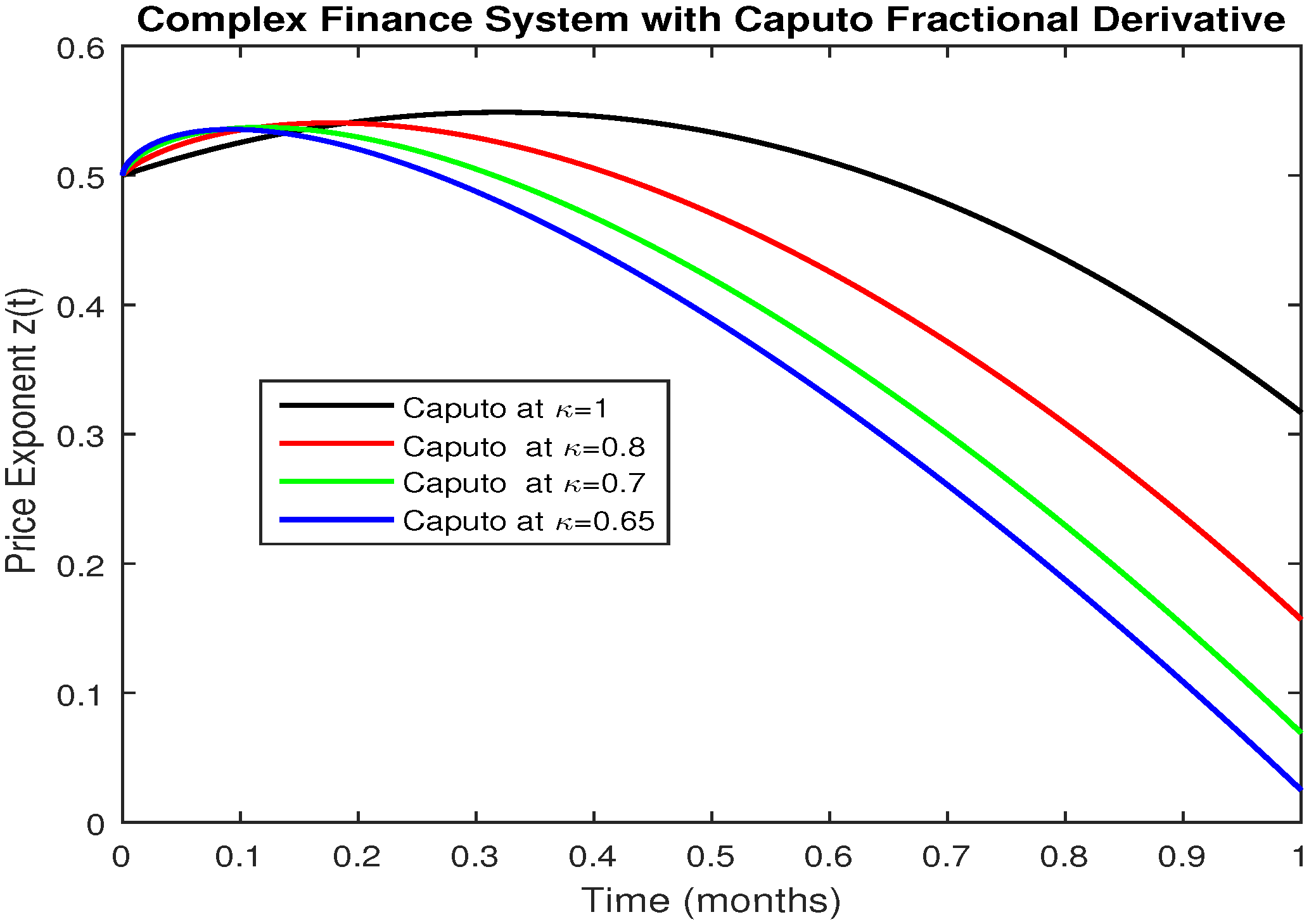
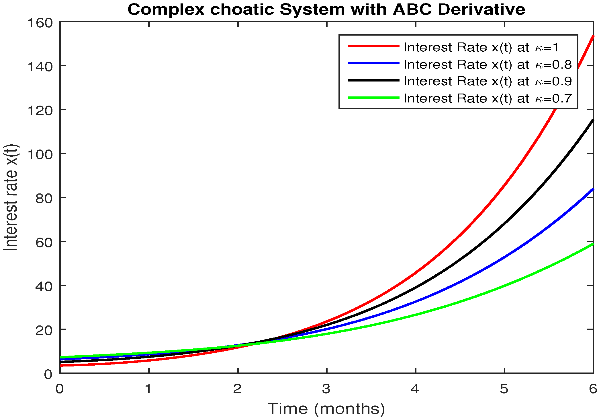
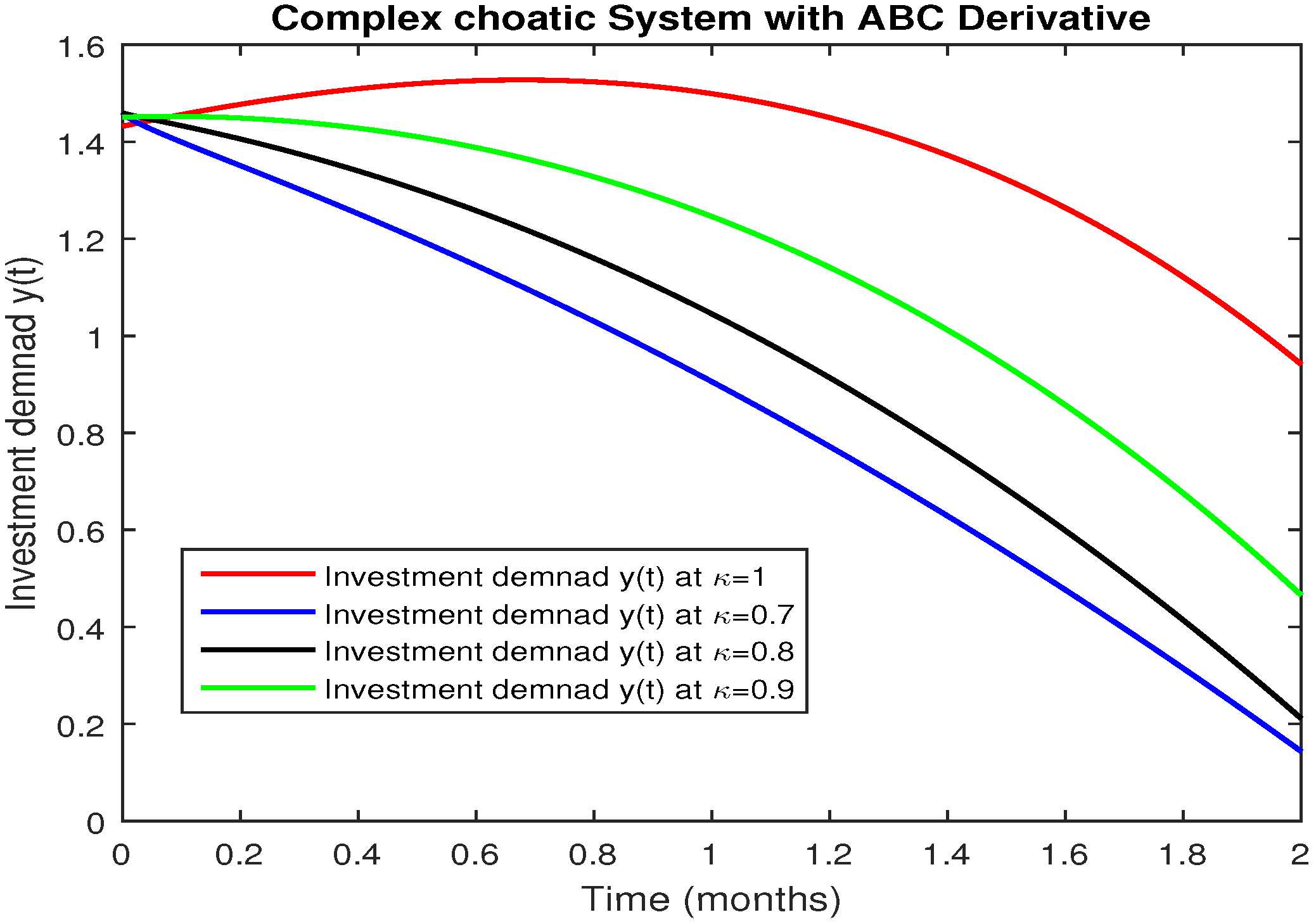
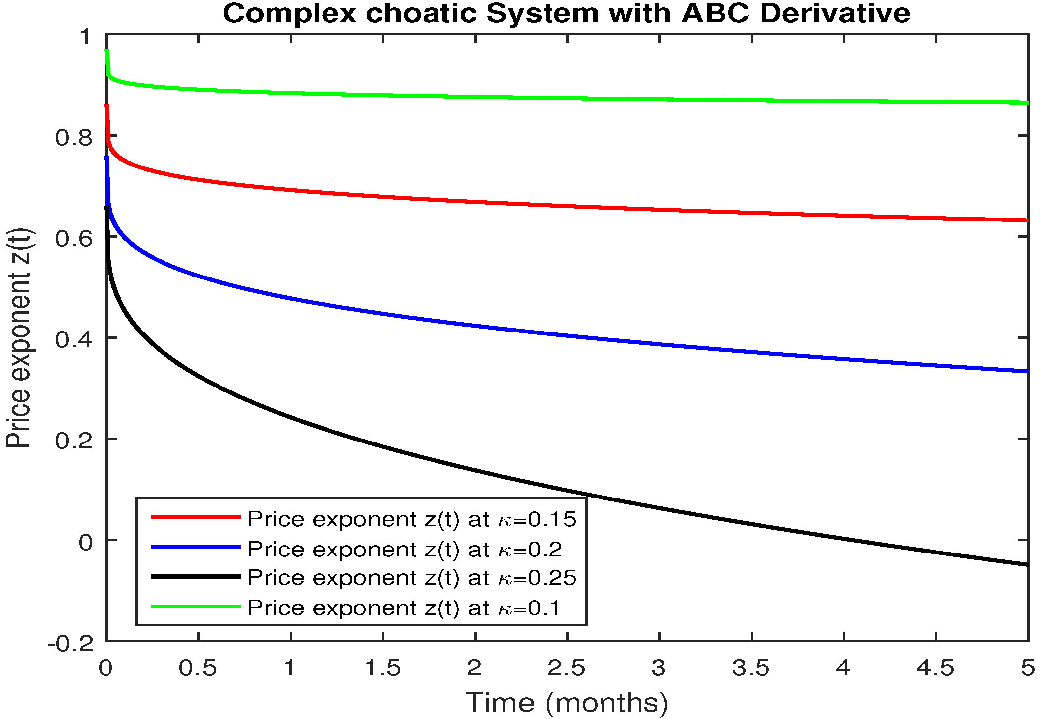
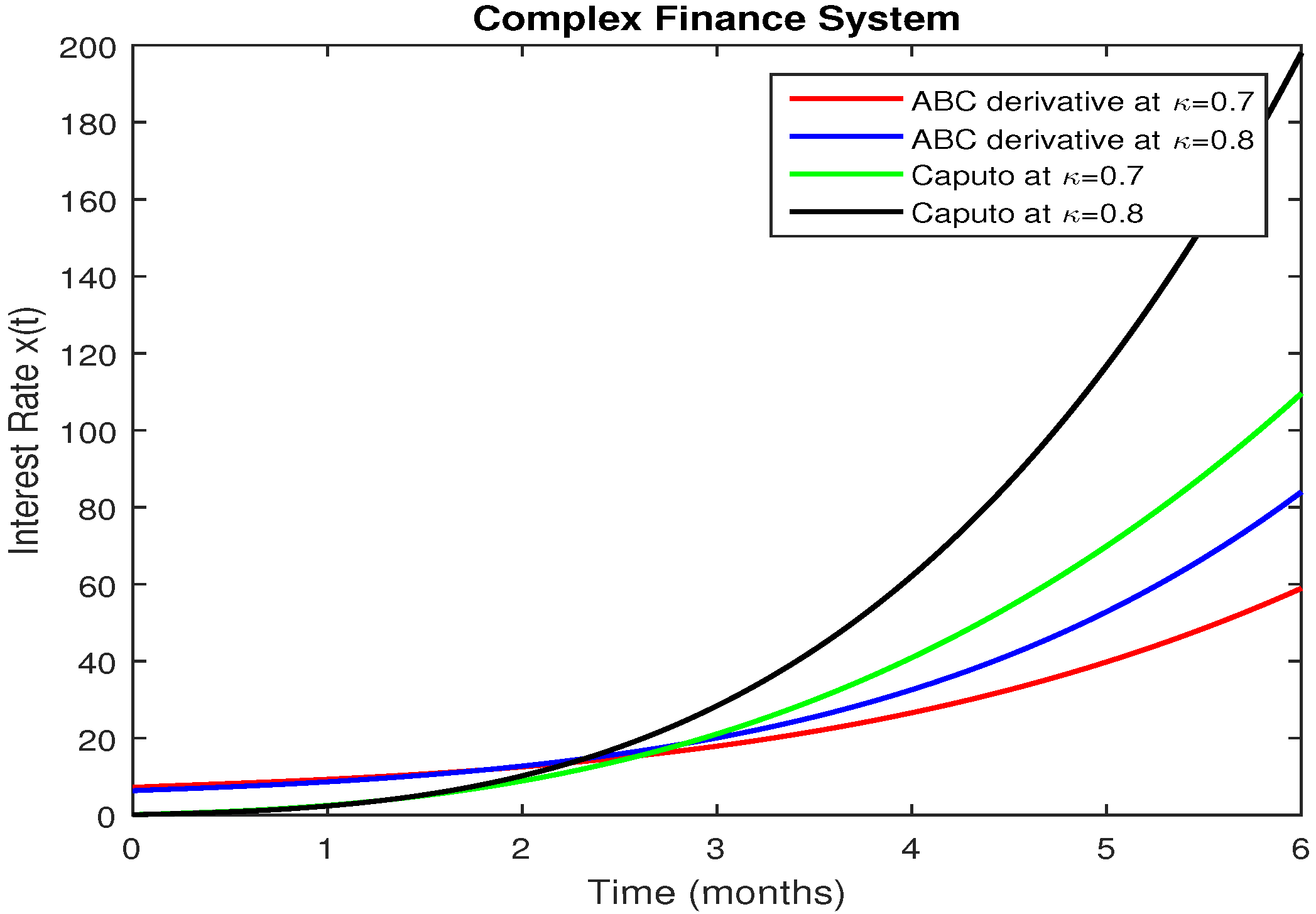
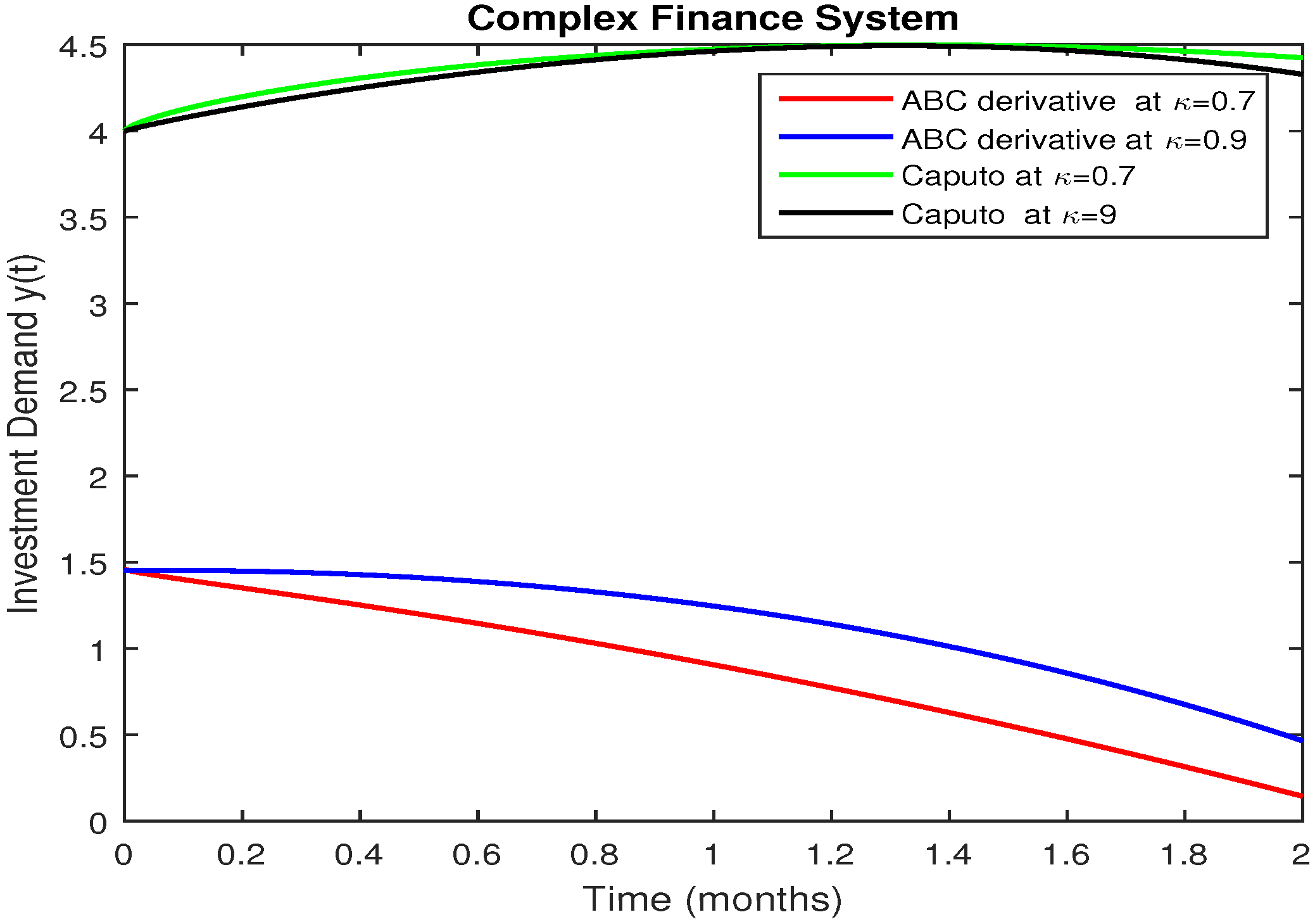
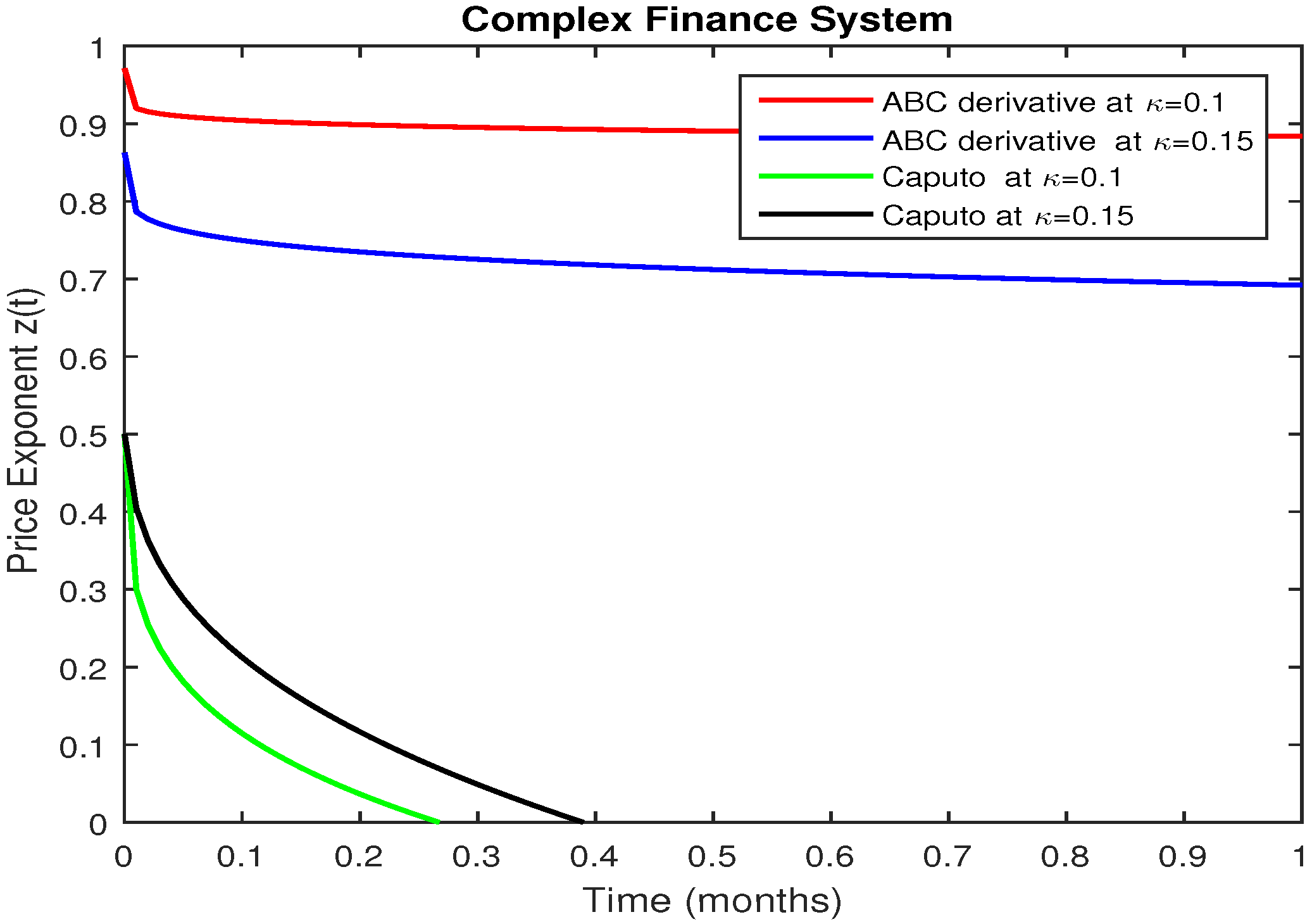
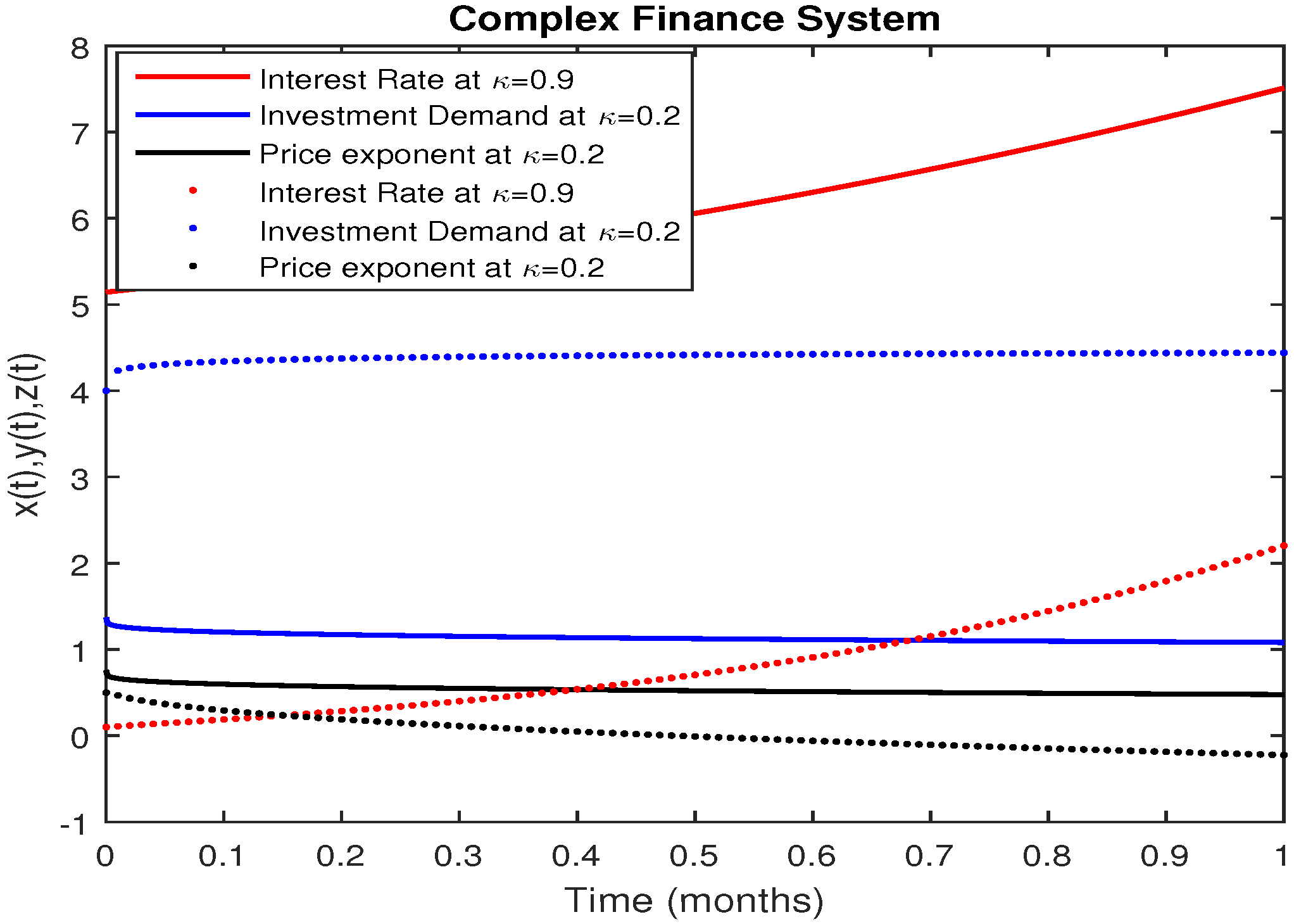
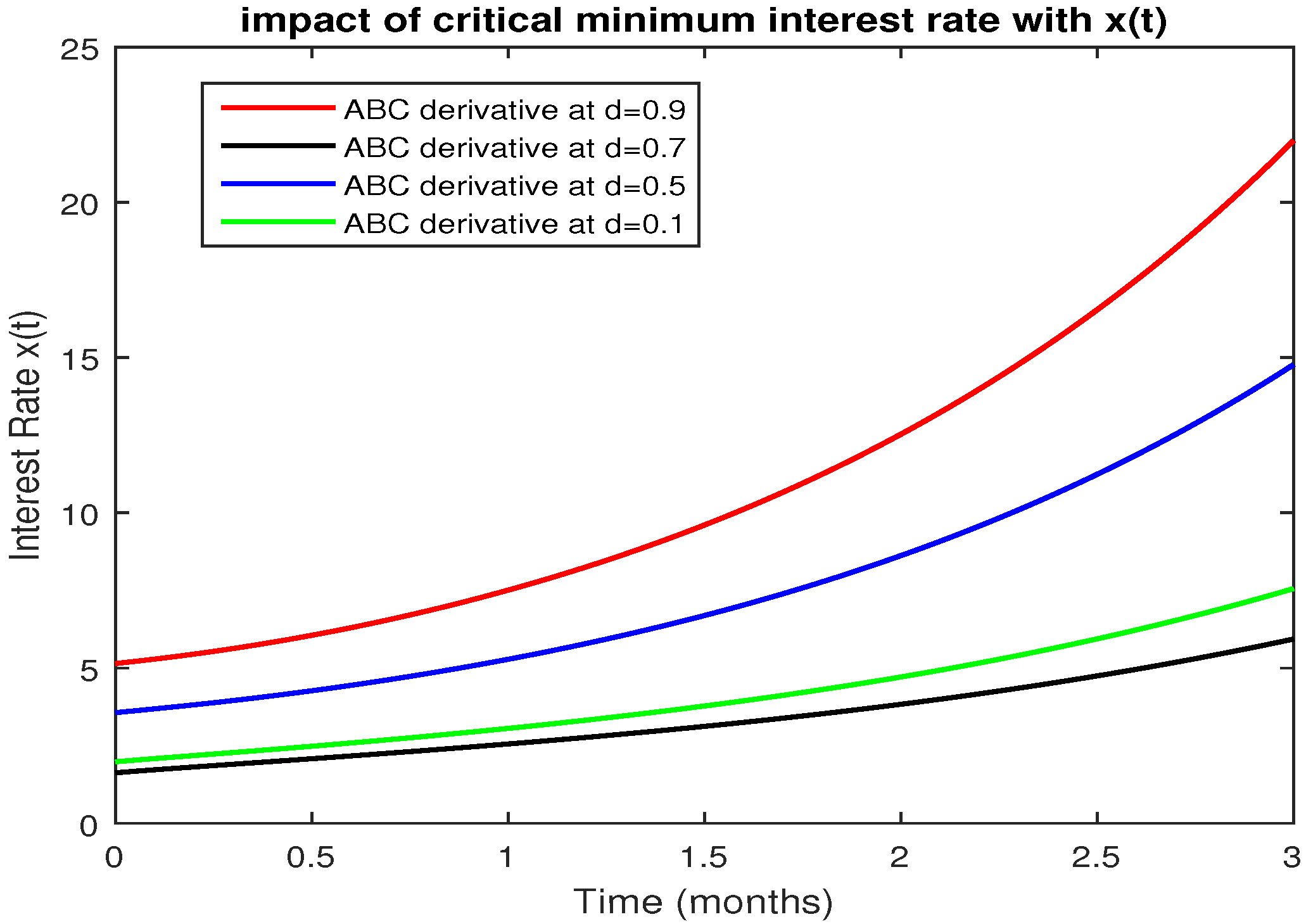
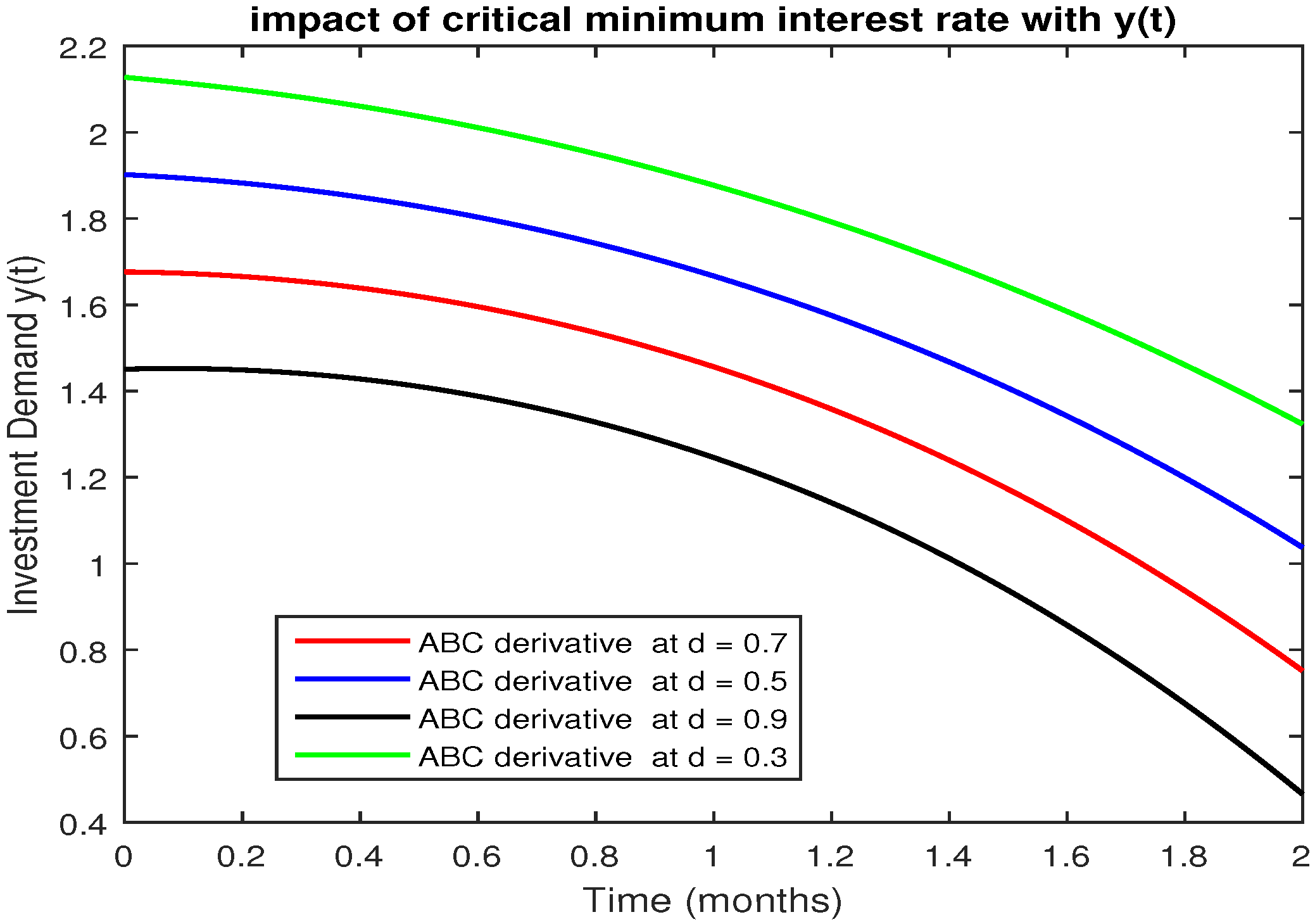
The ABC derivative has been used to present the theoretical solution of the fractional-order model consisting of a nonlinear system of the fractional differential equation. In this model, we represent x ( t ) , y ( t ) and z ( t ) are interest rate, investment demand, and price exponent with initial conditions x ( 0 ) = 0.1 , y ( 0 ) = 4 and z ( 0 ) = 0.5 , while the parameter a is for savings, b is to cost per investment, and c is the commercial markets demand elasticity with a = 3, b = 0.1, and c = 1 are given in [30,32]. By utilizing Caputo and ABC fractional derivative, the numerical results of interest rate, investment demand, and price exponent for various fractional estimations of η are acquired. Figure 1, Figure 2 and Figure 3 refer to the graphical solution of the finance system with the Caputo derivative of the finance system. Within this figure, we noticed that interest rate, investment demand, and the price exponent have more degree of freedom as contrasted with ordinary derivatives. From Figure 4, Figure 5 and Figure 6, we use ABC fractional-order derivative of the financial system, we effectively have seen that interest rate, investment demand, and price exponent rates are the better estimations compared with ordinary derivatives. Figure 7, Figure 8, Figure 9 and Figure 10 present the comparison of Caputo derivative and ABC derivative for the finance system. It should be observed that the behavior of the finance system is almost the same but ABC derivative presents more convenient and comfortable behavior in a system for closed-loop design. Caputo and ABC fractional derivatives are increasing or decreasing in the relationship between these variables. From Figure 1, Figure 2, Figure 3, Figure 4, Figure 5, Figure 6, Figure 7, Figure 8, Figure 9 and Figure 10, remarkable responses are obtained from the developed model for compartments by taking non-integer fractional parameter values. Numerical results show that the system keeps the η chaotic motion. The interest rate begins to rise according to initial conditions as investment demand and price exponent begin to fall, which shows the financial system’s actual macroeconomic behavior. It is observed here that a complex chaotic fractional system provides more appropriate and reliable results compared to time integer parameters for non-integer time-fractional parameters. In this system, we add parameter d to develop the new financial stable model which is the critical minimum interest rate. In order to observe the impact of factors on the mechanics of the fractional-order model, different numerical ways can be observed in Figure 11, Figure 12 and Figure 13. These simulations reveal a change in the value of a critical minimum interest rate of the model. We see that decreasing the critical minimum interest rate decreases the price of the exponent and the investment demand becomes high. Due to increasing the investment demand, our economy will become stronger.

6. Conclusions

This paper uses a dynamic chaotic fractional order model with an ABC derivative to conduct the economic system. The basis of this fractional model consists of exponentially decreasing non-singular kernels that appear in the derivation of the ABC. The financial model is presented with theoretical and numerical investigation. This demonstrates the regulation of the economic system’s critical minimum interest rate. In order to control the economic system, we are discussing a fractional order financing model. The modified model with ABC derivative shows a good financial system control agreement. The model offers the effect of evaluating numerical results on a critical minimum interest rate. Graphical representation shows the impact on the amount of critical minimum interest rate for variables with time. We can observe κ = 1 revealing more absorbing characteristics by numerical simulation using ABC non-integer order derivative. For interest rate, investment demand and price exponent, the concept of this research provides important results. Therefore, we conclude that the ABC derivative is useful to control and maintain the finance system to overcome the risk factors. The interest rate begins to rise according to initial conditions as investment demand and price exponent begin to fall, which shows the actual macroeconomic behavior of the financial system. It is observed here that the complex chaotic fractional system provides more appropriate and reliable results as compared to time integer parameters for non-integer time-fractional parameters.

Author Contributions

Conceptualization, M.F. and A.A. (Ali Akgül); Methodology, A.A. (Ali Akgül); Software, S.I.; Validation, A.H., A.A. (Aqeel Ahmad) and D.B.; Formal Analysis, D.B.; Investigation, A.A. (Aqeel Ahmad); Resources, A.A. (Aqeel Ahmad); Data Curation, M.F.; Writing-Original Draft Preparation, M.F.; Writing-Review & Editing, M.F.; All authors have read and agreed to the published version of the manuscript.

Funding

This research received no external funding.

Conflicts of Interest

The authors declare no conflict of interest.

References

  1. Neumaier, A. Mathematical Modelling. Available online: http://www.mat.univie.ac.at/~neum/ms/model.pdf (accessed on 18 January 2011).
  2. Merton, R.C.; Simons, R.V.; Wilkie, A.D. Influence of mathematical models in finance on practice: Past, present and future. Philos. Trans. Phys. Sci. Eng. 1994, 347, 451–463. [Google Scholar]
  3. Karatzas, I. Lectures on the Mathematics of Finance 8; American Mathematical Society: Providence, RI, USA, 1997. [Google Scholar]
  4. Hilfer, R. Applications of Fractional Calculus in Physics; World Scientific: Singapore, 2000; pp. 87–130. [Google Scholar]
  5. Kumar, D.; Singh, J.; Baleanu, D. Modified Kawahara equation within a fractional derivative with non-singular kernel. Therm. Sci. 2017, 22, 789–796. [Google Scholar] [CrossRef]
  6. Kumar, D.; Singh, J.; Baleanu, D.; Sushila. Analysis of regularized long-wave equation associated with a new fractional operator with Mittag–Leffler type kernel. Physica A 2018, 492, 155–167. [Google Scholar] [CrossRef]
  7. Baleanu, D.; Jajarmi, A.; Hajipour, M. A new formulation of the fractional optimal control problems involving Mittag–Leffler nonsingular kernel. J. Optim. Theory Appl. 2017, 175, 718–737. [Google Scholar] [CrossRef]
  8. Baleanu, D.; Jajarmi, A.; Asad, J.H.; Blaszczyk, T. The motion of a bead sliding on a wire in fractional sense. Acta Phys. Pol. A 2017, 131, 1561–1564. [Google Scholar] [CrossRef]
  9. Jajarmi, A.; Hajipour, M.; Baleanu, D. New aspects of the adaptive synchronization and hyperchaos suppression of a financial model. Chaos Solitons Fractals 2017, 99, 285–296. [Google Scholar] [CrossRef]
  10. Kilbas, A.A.; Srivastava, H.M.; Trujillo, J.J. Theory and Applications of Fractional Differential Equations; Elsevier: Amsterdam, The Netherlands, 2006. [Google Scholar]
  11. Baleanu, D.; Guvenc, Z.B.; Machado, J.A.T. New Trends in Nanotechnology and Fractional Calculus Applications; Springer: Dordrecht, The Netherlands, 2000. [Google Scholar]
  12. Yang, X.J.; Srivastava, H.M.; Machado, J.A.T. A new fractional derivative without singular kernel: Application to the modelling of the steady heat flow. Therm. Sci. 2016, 20, 753–756. [Google Scholar] [CrossRef]
  13. Caputo, M.; Fabrizio, M. A new definition of fractional derivative without singular kernel. Prog. Fract. Differ. Appl. 2015, 1, 73–85. [Google Scholar]
  14. Atangana, A. On the new fractional derivative and application to nonlinear Fisher’s reaction diffusion equation. Appl. Math. Comput. 2016, 273, 948–956. [Google Scholar] [CrossRef]
  15. Panda, S.K.; Karapınar, E.; Atangana, A. A numerical schemes and comparisons for fixed point results with applications to the solutions of Volterra integral equations in dislocated extended b a metric space. Alex. Eng. J. 2020, 59, 815–827. [Google Scholar] [CrossRef]
  16. Yavuz, M.; Özdemir, N. European vanilla option pricing model of fractional order without singular kernel. Fractal Fract. 2018, 2, 3. [Google Scholar] [CrossRef] [Green Version]
  17. Keten, A.; Yavuz, M.; Baleanu, D. Nonlocal Cauchy problem via a fractional operator involving power kernel in Banach Spaces. Fractal Fract. 2019, 3, 27. [Google Scholar] [CrossRef] [Green Version]
  18. Yavuz, M.; Abdeljawad, T. Nonlinear regularized long-wave models with a new integral transformation applied to the fractional derivative with power and Mittag–Leffler kernel. Adv. Differ. Equ. 2020, 2020, 367. [Google Scholar] [CrossRef]
  19. Yavuz, M.; Ozdemir, N.; Baskonus, H.M. Solutions of partial differential equations using the fractional operator involving Mittag–Leffler kernel. Eur. Phys. J. Plus 2018, 133, 215. [Google Scholar] [CrossRef]
  20. Gao, W.; Baskonus, H.M.; Shi, L. New investigation of Bats-Hosts Reservoir-People coronavirus model and apply to 2019-nCoV system. Adv. Differ. Equ. 2020, 2020, 1–11. [Google Scholar]
  21. Gao, W.; Veeresha, P.; Prakasha, D.G.; Baskonus, H.M. Novel dynamical structures of 2019-nCoV with nonlocal operator via powerful computational technique. Biology 2020, 9, 107. [Google Scholar] [CrossRef]
  22. Gao, W.; Veeresha, P.; Baskonus, H.M.; Prakasha, D.G.; Kumar, P. A new study of unreported cases of 2019-nCOV epidemic outbreaks. Chaos Solitons Fractals 2020, 138, 109929. [Google Scholar] [CrossRef]
  23. MoralesDelgadoa, V.F.; Aguilarb, J.F.; Taneco, M.A.; Escobar, R.F. Mathematical modeling of the smoking dynamics using fractional differential equations with local and nonlocal kernel. J. Nonlinear Sci. Appl. 2018, 11, 994–1014. [Google Scholar] [CrossRef] [Green Version]
  24. Atangana, A.; Baleanu, D. New fractional derivatives with nonlocal and non Singular Kernel: Theory and Application to Heat Transfer Model. Therm. Sci. 2016, 20, 763–769. [Google Scholar] [CrossRef] [Green Version]
  25. Kumar, S.; Kumar, A.; Argyros, I.K. A new analysis for the Keller-Segel model of fractional order. Numer. Algorithms 2017, 75, 213–228. [Google Scholar] [CrossRef]
  26. Kumar, S.; Rashidi, M.M. New analytical method for gas dynamic equation arising in shock fronts. Comput. Phys. Commun. 2014, 185, 1947–1954. [Google Scholar] [CrossRef]
  27. Odibat, Z.; Bataineh, A.S. An adaptation of homotopy analysis method for reliable treatment of strongly nonlinear problems: Construction of homotopy polynomials. Math. Methods Appl. Sci. 2015, 38, 991–1000. [Google Scholar] [CrossRef]
  28. Ma, J.H.; Chen, Y.S. Study for the bifurcation topological structure and the global complicated character of a kind of nonlinear finance system, I. Appl. Math. Mech. 2011, 22, 1240–1251. [Google Scholar] [CrossRef]
  29. Singh, J.; Kumar, D.; Al Qurashi, M.; Baleanu, D. A new fractional model for giving up smoking dynamics. Adv. Differ. Equ. 2017, 2017, 88. [Google Scholar] [CrossRef] [Green Version]
  30. Li, C.P.; Tao, C.X. On the fractional Adams method. Comput. Math. Appl. 2009, 58, 1573–1588. [Google Scholar] [CrossRef] [Green Version]
  31. Alkahtani, B.S.T. Chua’s circuit model with Atangana Baleanu derivative with fractional order. Chaos Solitons Fractals 2016, 89, 547–551. [Google Scholar] [CrossRef]
  32. Zhen, W.; Huang, X.; Shi, G. Analysis of nonlinear dynamics and chaos in a fractional-order financial system with time delay. Comput. Math. Appl. 2011, 62, 1531–1539. [Google Scholar]
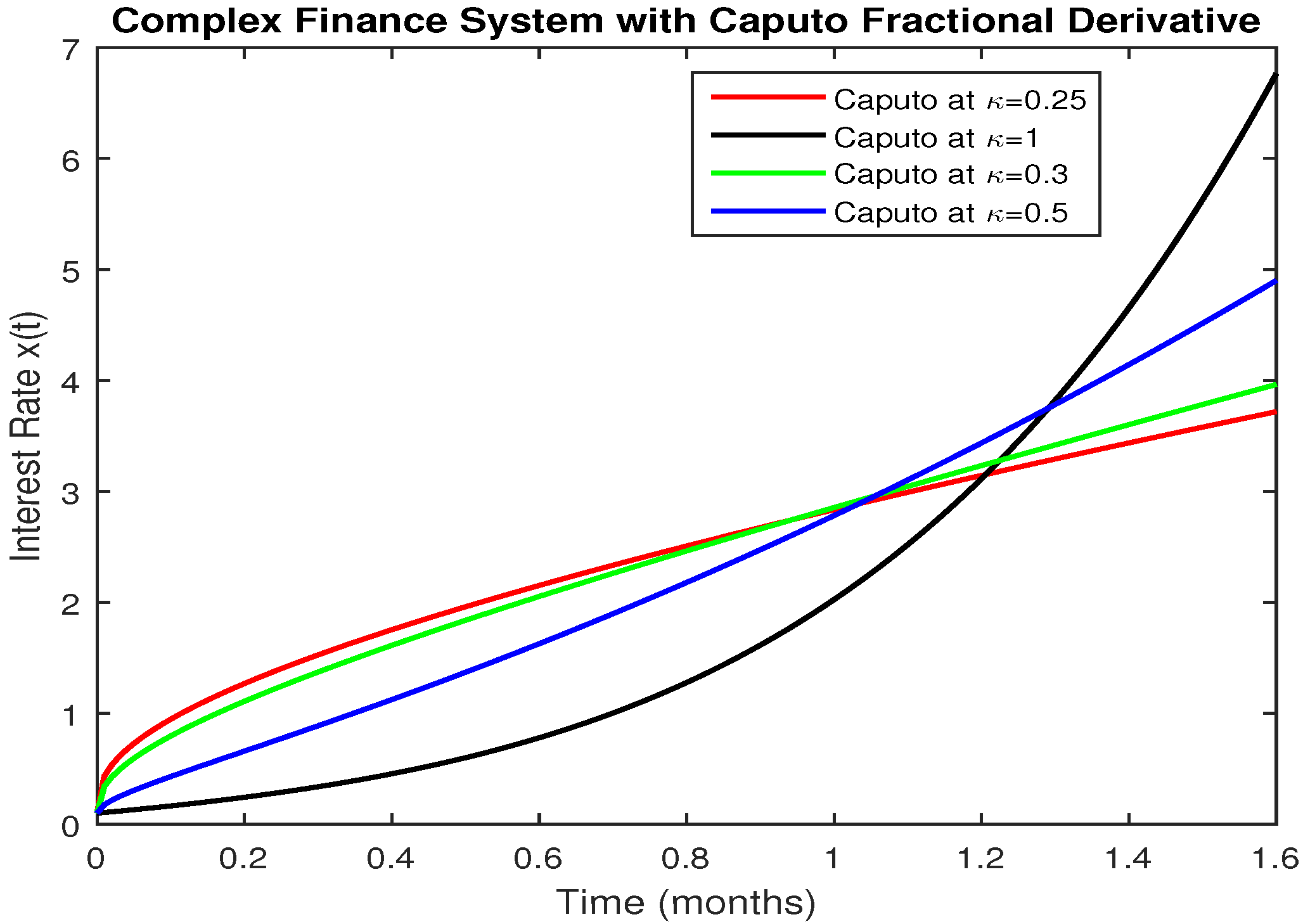
Figure 1. x ( t ) interest rate with Caputo fractional derivative.
Fractalfract 04 00043 g001
Figure 2. y ( t ) investment demand with Caputo fractional derivative.
Fractalfract 04 00043 g002
Figure 3. z ( t ) price exponent with Caputo fractional derivative.
Fractalfract 04 00043 g003
Figure 4. x ( t ) interest rate with ABC derivative.
Fractalfract 04 00043 g004
Figure 5. y ( t ) investment demand with ABC derivative.
Fractalfract 04 00043 g005
Figure 6. z ( t ) price exponent with ABC derivative.
Fractalfract 04 00043 g006
Figure 7. x ( t ) interest rate with Caputo and ABC derivative.
Fractalfract 04 00043 g007
Figure 8. y ( t ) investment demand with Caputo and ABC derivative.
Fractalfract 04 00043 g008
Figure 9. z ( t ) price exponent with Caputo and ABC derivative.
Fractalfract 04 00043 g009
Figure 10. z ( t ) price exponent with Caputo and ABC derivative.
Fractalfract 04 00043 g010
Figure 11. Impact of critical minimum interest rate with x ( t ) .
Fractalfract 04 00043 g011
Figure 12. Impact of critical minimum interest rate with y ( t ) .
Fractalfract 04 00043 g012
Figure 13. Impact of critical minimum interest rate with z ( t ) .
Fractalfract 04 00043 g013