Article

Numerical Solution of Fractional Order Burgers’ Equation with Dirichlet and Neumann Boundary Conditions by Reproducing Kernel Method

Faculty of Sciences, Department of Mathematics, Van Yuzuncu Yıl University, Van 65080, Turkey
*
Author to whom correspondence should be addressed.
Fractal Fract. 2020, 4(2), 27; https://doi.org/10.3390/fractalfract4020027
Submission received: 22 April 2020 / Revised: 14 June 2020 / Accepted: 16 June 2020 / Published: 19 June 2020

Abstract

:
In this research, obtaining of approximate solution for fractional-order Burgers’ equation will be presented in reproducing kernel Hilbert space (RKHS). Some special reproducing kernel spaces are identified according to inner products and norms. Then an iterative approach is constructed by using kernel functions. The convergence of this approach and its error estimates are given. The numerical algorithm of the method is presented. Furthermore, numerical outcomes are shown with tables and graphics for some examples. These outcomes demonstrate that the proposed method is convenient and effective.

1. Introduction

In this article, produced from a part of PhD thesis number 519846 from the Council of Higher Education, an iterative approach of reproducing kernel method (RKM) is considered for obtaining an approximate solution of the Burgers’ equation with fractional order as follows:
c D ξ α u ( z , ξ ) + c 1 ( z , ξ ) u z z ( z , ξ ) + c 2 ( z , ξ ) u ( z , ξ ) + c 3 ( z , ξ ) u z ( z , ξ ) + c 4 ( z , ξ ) u ( z , ξ ) u z ( z , ξ ) = f ( z , ξ ) 0 z 1 , 0 ξ 1 , 0 < α 1 ,
Here, c D ξ α is fractional differential operator in Caputo sense with respect to time variable ξ and also f ( z , ξ ) , c 1 ( z , ξ ) , c 2 ( z , ξ ) , c 3 ( z , ξ ) , c 4 ( z , ξ ) are continuous functions. For this model problem, initial-Neumann boundary conditions:
u ( z , 0 ) = 0 u z ( 0 , ξ ) = u z ( 1 , ξ ) = 0
and initial-Dirichlet boundary conditions:
u ( z , 0 ) = 0 u ( 0 , ξ ) = u ( 1 , ξ ) = 0
will be taken as above.
The Burgers’ equation is a simplified version of the Navier–Stokes equation. It was obtained by use of removing the pressure term from the Navier–Stokes equation by Burgers [1] in 1939. In other words, the Burgers’ equation can be expressed as a result of combining nonlinear wave motion with linear diffusion. Lately, many scientists have focused on Burgers’ equation by using several methods and different approaches. For instance, existence and uniqueness of local and global solution for Burgers’ equation was presented in [2] by Guesmia and Daili. Lombard and Matignon used a diffusive approximation for fractional-order Burgers’ equation in [3]. The averaging principle was proposed by Dong et al. for stochastic Burgers’ equation in [4]. Nojavan et al. obtained a numerical solution of Burgers’ equation by using discretization in reproducing kernel Hilbert space [5]. The Chebyshev wavelet method was developed by Oruc et al. for the numerical solution of time-fractional Burgers’ equation [6]. Pei et al. presented the local discontinuous Galerkin method for modified Burgers’ equation in [7]. The Petrov–Galerkin method was used by Roshan and Bhamra for modified Burgers’ equation in [8]. The collocation method was presented by Ramadan and Danaf for modified Burgers’ equation in [9]. Bahadir and Saglam constructed a mixed method for one dimensional Burgers’ equation [10]. Dag et al. used the cubic B-splines method [11]. Caldwell et al. proposed a finite element approximation for Burgers’ equation [12]. A finite difference method was used by Kutluay et al. for one-dimensional Burgers’ equation [13]. An approximate solution obtained by using the reproducing kernel method for Burgers’ equation [14]. A hybrid technique for the unsteady flow of a Burgers’ fluid is given by Raza et al. [15]. Laplace and finite Hankel transformations were proposed by Safdar et al. for generalized Burgers’ fluid with fractional derivative [16]. Time-fractional coupled Burgers’ equations were solved with generalized differential transform method by Liu and Hou [17]. Zhang et al proposed an analytical and numerical approach for multi-term time-fractional Burgers’ fluid model [18]. The Adomian decomposition method was applied to space-and time-fractional Burgers’ equation by Momani [19]. A generalized Taylor series technique was proposed by Ajou et al. for fractional nonlinear KdV-Burgers’ equation [20]. Mittal and Arora presented a numerical approach by using cubic B-spline functions for coupled viscous Burgers’ equation [21]. Jiwari used a hybrid numerical scheme for Burgers’ equation [22]. Kutluay et al. proposed a B-spline finite element method for Burgers’ equation [23].
Reproducing kernel concept is introduced by Zaremba [24]. In his study, Zaremba focused on the boundary value problem, which includes the Dirichlet boundary condition. Furthermore, the theoretical concept of reproducing kernel is developed in [25,26]. Reproducing kernel spaces of polynomial and trigonometric functions are constructed in [27]. Many studies have been conducted by using reproducing kernel method. For instance, eighth order boundary value problems [28], fractional advection-dispersion equation [29], fractional order systems of Dirichlet function types [30], fractional order Bagley–Torvik equation [31], time fractional telegraph equation [32], a local reproducing kernel method for Burgers’ equation [33], time-fractional partial integro differential equations [34], Riccati differential equations [35], nonlinear hyperbolic telegraph equation [36], time-fractional Tricomi and Keldysh equations [37], one-dimensional sine–Gordon equation [38], reaction-diffusion equations [39], integro differential equations of Fredholm operator type [40], fredholm integro-differential equations [41], nonlinear system of PDEs [42], class of fractional partial differential equation [43], Bagley–Torvik and Painlevé equations [44], nonlinear coupled Burgers equations [45] and so on [46,47,48,49,50,51,52,53,54,55,56,57,58,59].
This research is organized as: Specific definitions and Hilbert spaces are demonstrated in Section 2. Reproducing kernel solution is identified by RKM in Section 3. Convergence analysis of the approximate solution is proved in Section 4. Error estimation of the method is presented in Section 5. Two examples of fractional order Burgers’ equation are examined by the RKM and the algorithm of the process is given in Section 6. Finally, a short conclusion is given in Section 7.
The notation table Table 1 is given as follow:

2. Some Specific Definitions and Hilbert Spaces

In this section, some basic definitions and significant reproducing kernel spaces will be given.
Definition 1.
([58,59]) Fractional α order Caputo derivative is defined as:
c D ξ α u ( z , ξ ) = 1 Γ ( n α ) 0 ξ r u ( z , r ) ( ξ r ) 1 + α n d r , n 1 < α n , ξ > 0 .
Definition 2.
Let H be Hilbert space and T an abstract set. If following conditions are provide, then S : T × T C is is called as reproducing kernel function:
i . S ( . , τ ) H , τ T , i i . μ ( . ) , S ( . , τ ) = μ ( τ ) , τ T , μ H .

2.1. Reproducing Kernel Spaces with One Variable

In this subsection, reproducing kernel functions will be presented for some special Hilbert spaces. Definitions and kernel functions of these spaces will be given for z and ξ variables. W 2 n [ a , b ] shows the general reproducing kernel space for one variable. Equations (1) and (2a,b) has second order derivative for z and first order derivative for ξ . Therefore, the kernel function of W 2 3 [ 0 , 1 ] will be given for u z z and the kernel function of W 2 2 [ 0 , 1 ] will be given for u ξ . Furthermore, W 2 1 [ 0 , 1 ] space will be given for general function (without derivative). For the obtaining procedure of reproducing kernel functions, please see [47].
W 2 1 [ 0 , 1 ] Hilbert space
W 2 1 [ 0 , 1 ] = { g ( z ) | g is absolutely continuous function , g L 2 [ 0 , 1 ] } .
  • The inner product of W 2 1 0 , 1 can be taken as follows:
    g z , f z W 2 1 = g 0 f 0 + 0 1 g z f z d z .
  • The norm of W 2 1 0 , 1 can be taken as follows:
    g W 2 1 2 = g , g W 2 1 , g , f W 2 1 0 , 1 .
  • The kernel function of W 2 1 0 , 1 is as follows:
    R τ { 1 } z = 1 + z , z τ , 1 + τ , τ > z .
W 2 2 [ 0 , 1 ] Hilbert Space
W 2 2 [ 0 , 1 ] = { g ( ξ ) | g , g are absolutely continuous functions , g L 2 [ 0 , 1 ] , g ( 0 ) = 0 } .
Here, L 2 0 , 1 = { g 0 1 g 2 ξ d ξ < } .
  • The inner product of W 2 2 0 , 1 can be taken as follows:
    g ξ , f ξ W 2 2 = g 0 f 0 + g 0 f 0 + 0 1 g ξ f ξ d ξ .
  • The norm of W 2 2 [ 0 , 1 ] can be taken as follows:
    g W 2 2 2 = g , g W 2 2 , f , g W 2 2 0 , 1 .
  • The kernel function of W 2 2 [ 0 , 1 ] is as follows:
    R β { 2 } ξ = ξ β + 1 2 β ξ 2 1 6 ξ 3 , ξ β , 1 6 β 3 + 1 2 ξ β 2 + β ξ , ξ > β .
W 2 3 [ 0 , 1 ] Hilbert Space
W 2 3 [ 0 , 1 ] space with Dirichlet boundary condition:
W 2 3 [ 0 , 1 ] = { g ( z ) | g , g , g are absolutely continuous functions , g ( 3 ) L 2 [ 0 , 1 ] , g ( 0 ) = g ( 1 ) = 0 } .
  • The inner product of W 2 3 [ 0 , 1 ] can be taken as follows:
    g z , f z W 2 3 = g 0 f 0 + g 0 f 0 + g 1 f 1 + 0 1 g ( 3 ) z f ( 3 ) z d z .
  • The norm of W 2 3 [ 0 , 1 ] can be taken as follows:
    g W 2 3 2 = g , g W 2 3 , f , g W 2 3 0 , 1 .
  • The kernel function of W 2 3 [ 0 , 1 ] is as follows:
    R τ { 3 } ( z ) = 1 120 ( τ 1 ) z ( z τ 4 4 z τ 3 + 6 z τ 2 + τ z 4 5 τ z 3 120 τ z + 120 τ + z 4 ) , z τ , 1 120 ( z 1 ) τ ( τ z 4 4 τ z 3 + 6 τ z 2 + z τ 4 5 z τ 3 120 z τ + 120 z + τ 4 ) , z > τ .
W 2 3 [ 0 , 1 ] space with Neumann boundary condition:
  • The inner product of W 2 3 [ 0 , 1 ] can be taken as follows:
    g z , f z W 2 3 = g 0 f 0 + g 0 f 0 + g 0 f 0 + 0 1 g ( 3 ) z f ( 3 ) z d z .
  • The norm of W 2 3 [ 0 , 1 ] can be taken as follows:
    g W 2 3 2 = g , g W 2 3 , f , g W 2 3 0 , 1 .
  • The kernel function of W 2 3 [ 0 , 1 ] is as follows:
    For z τ , the kernel function:
    R τ { 3 } ( z ) = z ( 1 56 τ 4 1 14 τ 3 3 14 τ 2 + 4 7 τ ) + z 2 ( 1 7 τ 2 1 112 τ 4 1 28 τ 3 + 3 14 τ ) + z 3 ( 1 21 τ 2 + 1 336 τ 4 1 84 τ 3 1 14 τ ) + z 4 ( 1 1344 τ 4 + 1 36 τ 3 + 1 112 τ 2 1 42 τ ) + 1 120 z ,
    and for z > τ the kernel function:
    R τ { 3 } ( z ) = τ ( 1 56 z 4 1 14 z 3 3 14 z 2 + 4 7 z ) + τ 2 ( 1 7 z 2 1 112 z 4 1 28 z 3 + 3 14 z ) + τ 3 ( 1 21 z 2 + 1 336 z 4 1 84 z 3 1 14 z ) + τ 4 ( 1 1344 z 4 + 1 36 z 3 + 1 112 z 2 1 42 z ) + 1 120 τ

2.2. Reproducing Kernel Spaces for Two Variable

The problem (1) and (2a,b) has two variables z and ξ . For this reason, we should give the spaces, inner products, and kernel functions according to these variables. Because the highest order derivatives z and ξ to be considered, reproducing kernel spaces will be given for both z and ξ variables. The region which we consider is Θ = [ 0 , 1 ] × [ 0 , 1 ] . In this part, W 2 ( 3 , 2 ) ( Θ ) space is given for Dirichlet boundary conditions. These reproducing kernel spaces are also determined in the same way for Neumann boundary conditions.
W 2 ( 3 , 2 ) ( Θ ) Hilbert Space
W 2 ( 3 , 2 ) ( Θ ) = { u ( z , ξ ) | 3 u z 2 ξ is completely continuous in Θ , 5 u z 3 ξ 2 L 2 ( Θ ) , u ( z , 0 ) = u ( 0 , ξ ) = u ( 1 , ξ ) = 0 } .
  • The inner product of W 2 ( 3 , 2 ) ( Θ ) can be taken as follows:
    u ( z , ξ ) , v ( z , ξ ) W 2 ( 3 , 2 ) = i = 0 1 0 1 [ 2 ξ 2 i z i u ( 0 , ξ ) 2 ξ 2 i z i v ( 0 , ξ ) ] d ξ + 0 1 2 ξ 2 u ( 1 , ξ ) 2 ξ 2 v ( 1 , ξ ) d ξ + j = 0 1 j ξ j u ( z , 0 ) , j ξ j v ( z , 0 ) W 2 3 + 0 1 0 1 [ 3 z 3 2 ξ 2 u ( z , ξ ) 3 z 3 2 ξ 2 v ( z , ξ ) ] d z d ξ .
  • The norm of W 2 ( 3 , 2 ) ( Θ ) can be taken as follows:
    u W 2 ( 3 , 2 ) 2 = u , u W 2 ( 3 , 2 ) , u , v W 2 ( 3 , 2 ) ( Θ ) .
Theorem 1.
K ( τ , β ) ( z , ξ ) is the kernel function of W 2 ( 3 , 2 ) ( Θ ) and also it is obtained by multiplying kernel functions of W 2 3 [ 0 , 1 ] and W 2 2 [ 0 , 1 ] , respectively. So, it can be written that
K ( τ , β ) ( z , ξ ) = R τ { 3 } ( z ) R β { 2 } ( ξ ) .
For any u ( z , ξ ) W 2 ( 3 , 2 ) ( Θ )
u ( τ , β ) = u ( z , ξ ) , K ( τ , β ) ( z , ξ ) W 2 ( 3 , 2 )
and
K ( z , ξ ) ( τ , β ) = K ( τ , β ) ( z , ξ ) .
Proof. 
Inner product of W 2 ( 3 , 2 ) space (Equation (13)) will be used to prove the theorem.
u ( z , ξ ) , R τ { 3 } ( z ) R β { 2 } ( ξ ) ) W 2 ( 3 , 2 ) = j = 0 1 j ξ j u ( z , 0 ) , R τ { 3 } ( z ) j ξ j R β { 2 } ( 0 ) W 2 3 + i = 0 1 0 1 2 ξ 2 i z i u ( 0 , ξ ) 2 ξ 2 R β { 2 } ( x i ) i z i R τ { 3 } ( 0 ) d ξ + 0 1 2 ξ 2 u ( 1 , ξ ) R τ { 3 } ( 1 ) 2 ξ 2 R β { 2 } ( ξ ) d ξ + 0 1 0 1 3 z 3 2 ξ 2 u ( z , ξ ) 3 z 3 R τ { 3 } ( z ) 2 ξ 2 R β { 2 } ( ξ ) d z d ξ = 0 1 2 ξ 2 R β { 2 } ( ξ ) 2 ξ 2 0 1 3 z 3 u ( z , ξ ) 3 z 3 R τ { 3 } ( z ) d z + i = 0 1 i z i u ( 0 , ξ ) i z i R τ { 3 } ( 0 ) + u ( 1 , ξ ) R τ { 3 } ( 1 ) d ξ + j = 0 1 j ξ j u ( τ , 0 ) j ξ j R β { 2 } ( 0 ) = j = 0 1 j ξ j u ( τ , 0 ) j ξ j R β { 2 } ( 0 ) + 0 1 2 ξ 2 R β { 2 } ( ξ ) 2 ξ 2 u ( z , ξ ) , R τ { 3 } ( z ) W 2 3 d ξ = j = 0 1 j ξ j u ( τ , 0 ) j ξ j R β { 2 } ( 0 ) + 0 1 2 ξ 2 R β { 2 } ( ξ ) 2 ξ 2 u ( τ , ξ ) d ξ = u ( τ , ξ ) , R β { 2 } ( ξ ) W 2 2 = u ( τ , β ) .
So, u ( τ , ξ ) , R β { 2 } ( ξ ) = u ( τ , β ) , and
K ( τ , β ) ( z , ξ ) = K ( τ , β ) ( x , y ) , K ( z , ξ ) ( x , y ) W 2 ( 3 , 2 ) = K ( z , ξ ) ( x , y ) , K ( τ , β ) ( x , y ) W 2 ( 3 , 2 ) = K ( z , ξ ) ( τ , β ) .
Therefore, the proof is completed. □
W 2 ( 1 , 1 ) ( Θ ) Hilbert Space
W 2 ( 1 , 1 ) ( Θ ) = { u ( z , ξ ) | u is completely continuous in Θ , 2 u z ξ L 2 ( Θ ) } .
  • The inner product of W 2 ( 1 , 1 ) ( Θ ) can be taken as follows:
    u ( z , ξ ) , v ( z , ξ ) W 2 ( 1 , 1 ) = 0 1 [ ξ u ( 0 , ξ ) ξ v ( 0 , ξ ) ] d ξ + u ( z , 0 ) , v ( z , 0 ) W 2 1 + 0 1 0 1 [ z ξ u ( z , ξ ) z ξ v ( z , ξ ) ] d z d ξ
  • The norm of W 2 ( 1 , 1 ) ( Θ ) can be taken as follows:
    u W 2 ( 1 , 1 ) 2 = u , u W 2 ( 1 , 1 ) , u , v W 2 ( 1 , 1 ) ( Θ ) .
  • The kernel function of W 2 ( 1 , 1 ) ( Θ ) is as follows:
    K ˜ ( τ , β ) ( z , ξ ) = R τ { 1 } ( z ) R β { 1 } ( ξ ) .
Remark 1.
In the next sections all analysis will be given for the Dirichlet boundary conditions. A similar analysis can be made for Neumann boundary conditions.

3. Obtaining of Reproducing Kernel Solution for Equations (1) and (2a,b) in W 2 ( 3 , 2 ) ( Θ )

In the reproducing kernel method, an approximate solution will be obtained with the help of kernel function and linear operator L. The choosing of L is arbitrary. One can choose the whole linear part of the model problem or any linear part of it. Here, the whole linear part of the model problem is chosen as follow:
L : W 2 ( 3 , 2 ) ( Θ ) W 2 ( 1 , 1 ) ( Θ )
L u ( z , ξ ) = c D ξ α u + c 1 ( z , ξ ) u z z + c 2 ( z , ξ ) u + c 3 ( z , ξ ) u z .
The new statement of Equations (1)-(2a-2b) can be expressed as:
L u ( z , ξ ) = F ( z , ξ , u ( z , ξ ) , u z ( z , ξ ) ) , ξ , z [ 0 , 1 ]
and F ( z , ξ , u ( z , ξ ) , u z ( z , ξ ) ) = f ( z , ξ ) c 4 ( z , ξ ) u ( z , ξ ) u z ( z , ξ ) .
Let { ( z i , ξ i ) } i = 1 be a countable dense subset in Θ . Now, ψ i ( z , ξ ) basis function will be defined by applying the kernel function to the operator L.
ψ i ( z , ξ ) = L ( τ , β ) K ( τ , β ) ( z , ξ ) | ( τ , β ) = ( z i , ξ i ) = { c D t α K ( τ , β ) ( z , ξ ) + c 1 ( τ , β ) 2 x 2 K ( τ , β ) ( z , ξ ) + c 2 ( τ , β ) K ( τ , β ) ( z , ξ ) + c 3 ( τ , β ) x K ( τ , β ) ( z , ξ ) } | ( τ , β ) = ( z i , ξ i ) = 1 Γ ( 1 α ) 0 ξ i r K ( z , r ) ( z , ξ ) ( ξ i r ) α d r + c 1 ( z i , ξ i ) 2 x 2 K ( z i , ξ i ) ( z , ξ ) + c 2 ( z i , ξ i ) K ( z i , ξ i ) ( z , ξ ) + c 3 ( z i , ξ i ) x K ( z i , ξ i ) ( z , ξ ) , i = 1 , 2 ,
Now, it will be shown that ψ i ( z , ξ ) basis function belong to W 2 ( 3 , 2 ) ( Θ ) space and ψ i ( z , ξ ) satisfies the initial-boundary condition of W 2 ( 3 , 2 ) ( Θ ) space. For this purpose, the following theorem will be given.
Theorem 2.
The basis function ψ i ( z , ξ ) is belong to W 2 ( 3 , 2 ) ( Θ ) reproducing space for i = 1 , 2 , . . . .
Proof. 
To prove the theorem, we must show that the following conditions are provided.
  • It should be shown that 5 ψ i ( z , ξ ) z 3 ξ 2 L 2 ( Θ ) .
  • 3 ψ i ( z , ξ ) z 2 ξ is completely continuous function.
  • ψ i ( z , ξ ) basis function satisfies the initial and boundary conditions.
One can see that any elements of W 2 ( 3 , 2 ) ( Θ ) satisfy the above conditions. Now, the following equation can be written using the property of the kernel function K ( τ , β ) ( z , ξ )
τ 2 z 3 ξ 2 7 K ( τ , β ) ( z , ξ ) = τ 2 z 3 5 R τ { 3 } ( z ) ξ 2 2 R β { 2 } ( ξ ) .
Here, both τ 2 z 3 5 R τ { 3 } ( z ) and ξ 2 2 R β { 2 } ( ξ ) are continuous in [ 0 , 1 ] . These functions are bounded because they are continuous in [ 0 , 1 ] . So, it can be written
| τ 2 z 3 ξ 2 7 K ( τ , β ) ( z , ξ ) | M 1 .
In the same way, one can write that
| β z 3 ξ 2 6 K ( τ , β ) ( z , ξ ) | M 2 | z 3 ξ 2 5 K ( τ , β ) ( z , ξ ) | M 3 | τ z 3 ξ 2 6 K ( τ , β ) ( z , ξ ) | M 4 .
Here, M 1 , M 2 , M 3 and M 4 are positive constants. From (17),
| 5 ψ i ( z , ξ ) z 3 ξ 2 | | 1 Γ ( 1 α ) 0 ξ i M 2 ( ξ i r ) α d r + c 1 ( z i , ξ i ) M 1 + c 2 ( z i , ξ i ) M 3 + c 3 ( z i , ξ i ) M 4 | M 2 Γ ( 2 α ) ξ i 1 α + | c 1 ( z i , ξ i ) | M 1 + | c 2 ( z i , ξ i ) | M 3 + | c 3 ( z i , ξ i ) | M 4 .
Therefore, 5 ψ i ( z , ξ ) z 3 ξ 2 L 2 ( Θ ) . Furthermore, 3 ψ i ( z , ξ ) z 2 ξ is completely continuous in Θ since Θ is closed region. Finally, basis function ψ i ( z , ξ ) satisfies initial-boundary conditions such that K ( τ , β ) ( z , 0 ) = 0 and K ( τ , β ) ( 0 , ξ ) = K ( τ , β ) ( 1 , ξ ) = 0 . Therefore, ψ i ( z , ξ ) W 2 ( 3 , 2 ) ( Θ ) . □
Theorem 3.
{ ψ i ( z , ξ ) } i = 1 is a complete system in W 2 ( 3 , 2 ) ( Θ ) .
Proof. 
It is known that
ψ i ( z , ξ ) = ( L * φ i ) ( z , ξ ) = ( L * φ i ) ( τ , β ) , K ( z , ξ ) ( τ , β ) W 2 ( 3 , 2 ) = φ i ( τ , β ) , L ( τ , β ) K ( z , ξ ) ( τ , β ) W 2 ( 1 , 1 ) = L ( τ , β ) K ( z , ξ ) ( τ , β ) | ( τ , β ) = ( z i , ξ i ) = L ( τ , β ) K ( τ , β ) ( z , ξ ) | ( τ , β ) = ( z i , ξ i ) .
Clearly, for each fixed u ( z , ξ ) W 2 ( 3 , 2 ) ( Θ ) , if u ( z , ξ ) , ψ i ( z , ξ ) W 2 ( 3 , 2 ) = 0 then ψ i ( z , ξ ) W 2 ( 3 , 2 ) ( Θ ) , i = 1 , 2 , . Therefore,
u ( z , ξ ) , ( L * φ i ) ( z , ξ ) W 2 ( 3 , 2 ) = L u ( z , ξ ) , φ i ( z , ξ ) W 2 ( 1 , 1 ) = ( L u ) ( z i , ξ i ) = 0 , i = 1 , 2 ,
{ ( z i , ξ i ) } i = 1 is dense in Θ . Hence, ( L u ) ( z , ξ ) = 0 . By using of inverse operator L 1 , it can be seen that u = 0 . So, theorem is proven. □
The orthonormal basis system { ψ i ¯ ( z , ξ ) } i = 1 of W 2 ( 3 , 2 ) ( Θ ) can be obtained by the way of Gram–Schmidt orthogonalization process of { ψ i ( z , ξ ) } i = 1 as follow:
ψ i ¯ ( z , ξ ) = k = 1 i η i k ψ k ( z , ξ ) , i = 1 , 2 ,
In Equation (20), η i i > 0 and η i k are orthogonalization coefficients.
Theorem 4.
If { ( z i , ξ i ) } i = 1 is dense in Θ, then the solution (16) is
u ( z , ξ ) = i = 1 k = 1 i η i k F ( z k , ξ k , u ( z k , ξ k ) , z u ( z k , ξ k ) ) ψ ¯ i ( z , ξ ) .
Proof. 
It is known that { ψ i ( z , ξ ) } i = 1 system is complete in W 2 ( 3 , 2 ) ( Θ ) from the previous theorem. So, it can be written
u ( z , ξ ) = i = 1 u ( z , ξ ) , ψ ¯ i ( z , ξ W 2 ( 3 , 2 ) ψ ¯ i ( z , ξ ) = i = 1 k = 1 i η i k u ( z , ξ ) , ψ k ( z , ξ ) W 2 ( 3 , 2 ) ψ ¯ i ( z , ξ ) = i = 1 k = 1 i η i k u ( z , ξ ) , L * φ k ( z , ξ ) W 2 ( 3 , 2 ) ψ ¯ i ( z , ξ ) = i = 1 k = 1 i η i k L u ( z , ξ ) , φ k ( z , ξ ) W 2 ( 1 , 1 ) ψ ¯ i ( z , ξ ) = i = 1 k = 1 i η i k L u ( z , ξ ) , K ˜ ( z k , ξ k ) ( z , ξ ) W 2 ( 1 , 1 ) ψ ¯ i ( z , ξ ) = i = 1 k = 1 i η i k L u ( z k , ξ k ) ψ ¯ i ( z , ξ ) = i = 1 k = 1 i η i k F ( z k , ξ k , u ( z k , ξ k ) , z u ( z k , ξ k ) ) ψ ¯ i ( z , ξ ) .
So, theorem is proven. □
In Equation (21), u ( z , ξ ) is described as infinite term sum. In the next equation, finitely n-terms solution will be given as u n ( z , ξ ) :
u n ( z , ξ ) = i = 1 n k = 1 i η i k F ( z k , ξ k , u ( z k , ξ k ) , z u ( z k , ξ k ) ) ψ ¯ i ( z , ξ ) .

4. Convergence of Reproducing Kernel Solution

In this section, it will be shown that
u ( z , ξ ) u n ( z , ξ ) 0 as n .
If we take
A i = k = 1 i η i k F ( z k , ξ k , u ( z k , ξ k ) , z u ( z k , ξ k ) ) ,
then (21) can be described as
u ( z , ξ ) = i = 1 A i ψ ¯ i ( z , ξ ) .
Now, u ( z 1 , ξ 1 ) is found by taking ( z 1 , ξ 1 ) = 0 from the initial conditions of problem. Furthermore, by choosing u 0 ( z 1 , ξ 1 ) = u ( z 1 , ξ 1 ) , the n-term approximation to u ( z , ξ ) is expressed as follows:
u n ( z , ξ ) = i = 1 n B i ψ ¯ i ( z , ξ ) ,
here
B i = k = 1 i η i k F ( z k , ξ k , u k 1 ( z k , ξ k ) , z u k 1 ( z k , ξ k ) ) .
Now, some theoretical results will be given for convergence of F ( z n , ξ n , u n 1 ( z n , ξ n ) , z u n 1 ( z n , ξ n ) ) and u n ( z , ξ ) , respectively.
Lemma 1.
If F ( z , ξ , u ( z , ξ ) , u z ( z , ξ ) ) is continuous and u n u ^ for ( z n , ξ n ) ( τ , β ) , then
F ( z n , ξ n , u n 1 ( z n , ξ n ) , z u n 1 ( z n , ξ n ) ) F ( τ , β , u ^ ( τ , β ) , z u ^ ( τ , β ) ) .
Proof. 
Since
| u n 1 ( z n , ξ n ) u ^ ( τ , β ) | = | u n 1 ( z n , ξ n ) u n 1 ( τ , β ) + u n 1 ( τ , β ) u ^ ( τ , β ) | | u n 1 ( z n , ξ n ) u n 1 ( τ , β ) | + | u n 1 ( τ , β ) u ^ ( τ , β ) | .
Using reproducing kernel feature, it can be written that
u n 1 ( z n , ξ n ) = u n 1 ( z , ξ ) , K ( z n , ξ n ) ( z , ξ ) W 2 ( 3 , 2 ) , u n 1 ( τ , β ) = u n 1 ( z , ξ ) , K ( τ , β ) ( z , ξ ) W 2 ( 3 , 2 ) .
It follows that
| u n 1 ( z n , ξ n ) u n 1 ( τ , β ) | = | u n 1 ( z , ξ ) , K ( z n , ξ n ) ( z , ξ ) K ( τ , β ) ( z , ξ ) | .
It can be said that there exists M > 0 from the convergence of u n 1 ( z , ξ ) such that
u n 1 ( z , ξ ) W 2 ( 3 , 2 ) M u ^ ( τ , β ) W 2 ( 3 , 2 ) , as n M .
In a similar way, it can be proven
K ( z n , ξ n ) ( z , ξ ) K ( τ , β ) ( z , ξ ) W 2 ( 3 , 2 ) 0 , for n
by using Equation (14). So,
u n 1 ( z n , ξ n ) u ^ ( τ , β ) , as ( z n , ξ n ) ( τ , β ) .
In a similar way it can be shown that
z u n 1 ( z n , ξ n ) z u ^ ( τ , β ) , as ( z n , ξ n ) ( τ , β ) .
Therefore,
F ( z n , ξ n , u n 1 ( z n , ξ n ) , z u n 1 ( z n , ξ n ) ) F ( τ , β , u ^ ( τ , β ) , z u ^ ( τ , β ) ) .
So, lemma is proven. □
Theorem 5.
Assume that (16) has a unique solution, u n is a bounded and { ( z i , ξ i ) } i = 1 is dense in Θ. Then, u n ( z , ξ ) converges to u ( z , ξ ) and
u ( z , ξ ) = i = 1 B i ψ ¯ i ( z , ξ ) .
Proof. 
Firstly, we aim to show that u n ( z , ξ ) is convergence. Following equality can be written
u n + 1 ( z , ξ ) = u n ( z , ξ ) + B n + 1 ψ ¯ n + 1 ( z , ξ ) .
from the Equation (27). Using the orthonormality of { ψ ¯ i } i = 1 , we have
u n + 1 2 = u n 2 + B n + 1 2 = i = 1 n + 1 B i 2 .
Therefore, u n + 1 > u n satisfies from (40). Here, it seems that u n is bounded. So, one can know that u n is convergent. Therefore, there exists a constant b so that
i = 1 B i 2 = b .
So, above equation shows that { B i } i = 1 l 2 . If m > n , then
u m u n 2 = u m u m 1 + u m 1 u m 2 + + u n + 1 u n 2 = u m u m 1 2 + u m 1 u m 2 2 + + u n + 1 u n 2 .
The following equation is obtained
u m u m 1 2 = B m 2 ,
and consequently
u m u n 2 = l = n + 1 m B l 2 0 , as n .
The completeness of W 2 ( 3 , 2 ) ( Θ ) shows that u n u ^ for n . Next, it will be shown that u ^ is the representation solution of (16). If the limit is taken both sides of Equation (27), the following equation can be written:
u ^ ( z , ξ ) = i = 1 B i ψ ¯ i ( z , ξ ) .
Note that
( L u ^ ) ( z , ξ ) = i = 1 B i L ψ ¯ i ( z , ξ ) ,
( L u ^ ) ( z l , ξ l ) = i = 1 B i L ψ ¯ i ( z l , ξ l ) = i = 1 B i L ψ ¯ i ( z , ξ ) , φ l ( z , ξ ) W 2 ( 1 , 1 ) = i = 1 B i ψ ¯ i ( z , ξ ) , L * φ l ( z , ξ ) W 2 ( 3 , 2 ) = i = 1 B i ψ ¯ i ( z , ξ ) , ψ l ( z , ξ ) W 2 ( 3 , 2 ) .
Therefore,
l = 1 i η i l ( L u ^ ) ( z l , ξ l ) = i = 1 B i ψ ¯ i ( z , ξ ) , l = 1 i η i l ψ l ( z , ξ ) W 2 ( 3 , 2 )
= i = 1 B i ψ ¯ i ( z , ξ ) , ψ ¯ l ( z , ξ ) W 2 ( 3 , 2 ) = B l .
From (28), the following equation can be expressed
L u ^ ( z l , ξ l ) = F ( z l , ξ l , u l 1 ( z l , ξ l ) , z u l 1 ( z l , ξ l ) ) .
For each ( τ , β ) Θ , { ( z i , ξ i ) } i = 1 is dense in Θ . Therefore, there exists a subsequence { ( z n j , ξ n j ) } j = 1 such that ( z n j , ξ n j ) ( τ , β ) , j . It is known that
L u ^ ( z n j , ξ n j ) = F ( z n j , ξ n j , u n j 1 ( z n j , ξ n j ) , z u n j 1 ( z n j , ξ n j ) ) .
By using Lemma 1 and continuity of F, it can be seen that
( L u ^ ) ( τ , β ) = F ( τ , β , u ^ ( τ , β ) , z u ^ ( τ , β ) ) , for j .
Equation (52) implies that u ^ ( z , ξ ) satisfies Equation (16). So, proof is completed. □
Theorem 6.
z i i ξ j j u n ( z , ξ ) uniformly converges to z i i ξ j j u ( z , ξ ) for j = 0 , 1 and i = 0 , 1 , 2 .
Proof. 
The convergence of u n is given in the previous theorem. Now,
| z i i ξ j j u ( z , ξ ) z i i ξ j j u n ( z , ξ ) | = | u ( y , s ) u n ( y , s ) , z i i ξ j j L K ( z , ξ ) ( y , s ) | u u n z i i ξ j j L K ( z , ξ ) ( y , s ) C i , j u u n .
So,
| z i i ξ j j u n ( z , ξ ) z i i ξ j j u ( z , ξ ) | 0 as n .
 □

5. Error Estimation of Method

In this section, error analysis for the presented method will be given. In this analysis, one can understand that the error estimation varies depending on the selected step size. Now, the step size, chosen of points, and norm will be taken as follow:
z i = i h z , h z = 1 / n , ξ j = j h ξ , h ξ = 1 / n , i , j = 1 , , n .
u ( z , ξ ) = max | u ( z , ξ ) | for ( z , ξ ) Θ
Furthermore, u ( z , ξ ) u n ( z , ξ ) can be written in two ways for each variable as follow:
u ( z , ξ ) u n ( z , ξ ) = u ( z i , ξ ) u n ( z i , ξ ) + z i z ( τ u ( τ , ξ ) τ u n ( τ , ξ ) ) d τ
and
u ( z , ξ ) u n ( z , ξ ) = u ( z , ξ i ) u n ( z , ξ i ) + ξ i ξ ( β u ( z , β ) β u n ( z , β ) ) d β .
The following two theorems will be given for error estimation considering the two equations above.
Theorem 7.
Let u ( z , ξ ) u n ( z , ξ ) be error in W 2 ( 6 , 2 ) ( Θ ) . Therefore, there exist a C > 0 so that
u ( z , ξ ) u n ( z , ξ ) C ( h z 2 + h z h ξ ) .
Proof. 
For [ z i , z i + 1 ] × [ ξ j , ξ j + 1 ] Θ , the following equality can be written:
z u ( z , ξ ) z u n ( z , ξ ) = z u ( z , ξ ) z u ( z i , ξ j ) + z u n ( z i , ξ j ) z u n ( z , ξ ) + z u ( z i , ξ j ) z u n ( z i , ξ j )
Here, Taylor expansion will be used to show error estimate for the function z u ( z , ξ ) around the point ( z i , ξ j ) . This equality will be analyzed in three cases. It is known that
z u ( z , ξ ) = z u ( z i , ξ j ) + ( h z z + h ξ ξ ) z u ( z i + ϵ h z , ξ j + ϵ h ξ ) , ϵ [ 0 , 1 ] .
Firstly, the continuity of z 2 2 u ( z , ξ ) and z ξ 2 u ( z , ξ ) on Θ is considered. So, one can write that
z u ( z , ξ ) z u ( z i , ξ j ) = O ( h z + h ξ ) .
Secondly, one know that
| z u n ( z i , ξ j ) z u n ( z , ξ ) | z i z | y 2 2 u n ( y , ξ j ) | d y + ξ j ξ | z s 2 u n ( z , s ) | d s .
The next equation can be stated by using of maximum norm
z u n ( z i , ξ j ) z u n ( z , ξ ) = O ( h z + h ξ ) .
Finally, for sufficiently large n, any ε > 0 and using Theorem 6 such that
z u ( z i , ξ j ) z u n ( z i , ξ j ) < ε .
From Equation (54), it is known that ε is arbitrary constant and the chosen of n, the following equality can be expressed
z u ( z i , ξ j ) z u n ( z i , ξ j ) = O ( h z + h ξ ) .
In light of the information given above, error estimation will be given as follows:
u ( z , ξ ) u n ( z , ξ ) = u ( z i , ξ ) u n ( z i , ξ ) + z i z ( y u ( y , ξ ) y u n ( y , ξ ) ) d y
u ( z , ξ ) u n ( z , ξ ) u ( z i , ξ ) u n ( z i , ξ ) + z i z y u ( y , ξ ) y u n ( y , ξ ) d y C ( h z 2 + h ξ h z ) .
 □
So far, error estimation analysis is done for z variable. The error estimation analysis for variable ξ will be given by the next theorem.
Theorem 8.
Assume that z 3 3 ξ u ( z , ξ ) and z 2 2 ξ 2 2 u ( z , ξ ) are continuous and also, z 3 3 ξ u ( z , ξ ) and z 2 2 ξ 2 2 u ( z , ξ ) are bounded. So, there exist a C > 0 such that the error estimate can be expressed as:
u n ( z , ξ ) u ( z , ξ ) C ( h ξ h z 3 + h ξ 2 h z 2 ) .
Proof. 
For [ z i , z i + 1 ] × [ ξ i , ξ i + 1 ] Θ , it can be written
z 2 2 ξ u ( z , ξ ) z 2 2 ξ u n ( z , ξ ) = z 2 2 ξ u ( z , ξ ) z 2 2 ξ u ( z i , ξ j ) + z 2 2 ξ u n ( z i , ξ j ) z 2 2 ξ u n ( z , ξ ) + z 2 2 ξ u ( z i , ξ j ) z 2 2 ξ u n ( z i , ξ j ) .
Taylor series expansion for z 2 2 ξ u ( z , ξ ) function around the point ( z i , ξ j ) as follow:
z 2 2 ξ u ( z , ξ ) = z 2 2 ξ u ( z i , ξ j ) + ( h z z + h ξ ξ ) z 2 2 ξ u ( z i + h z ϵ , ξ j + h ξ ϵ ) + . . . , ϵ [ 0 , 1 ] .
Firstly, the following expression can be written by considering the continuation of z 3 3 ξ u ( z , ξ ) and z 2 2 ξ 2 2 u ( z , ξ ) on Θ ,
z 2 2 ξ u ( z , ξ ) z 2 2 ξ u ( z i , ξ j ) = O ( h z + h ξ ) .
Secondly, one knows that
| z 2 2 ξ u n ( z i , ξ j ) z 2 2 ξ u n ( z , ξ ) | z i z | y 3 3 ξ u n ( y , ξ j ) | d y + ξ i ξ | z 2 2 s 2 2 u n ( z , s ) | d s .
The follow equality can be written by using of maximum norm:
z 2 2 ξ u n ( z i , ξ j ) z 2 2 ξ u n ( z , ξ ) = O ( h z + h ξ ) .
The following statement can be written using Theorem 6 and for any arbitrary ε > 0 , and sufficiently large n:
z 2 2 ξ u ( z i , ξ j ) z 2 2 ξ u n ( z i , ξ j ) < ε .
The following equation can be written from Equation (55) by choosing of n and using arbitrary constant ε . So, we have
z 2 2 ξ u ( z , ξ ) z 2 2 ξ u n ( z , ξ ) = O ( h z + h ξ ) .
One can know that the following equations can be written from the integral property for differentiable functions:
z ξ u ( z , ξ ) z ξ u n ( z , ξ ) = z ξ u ( z i , ξ ) z ξ u n ( z , ξ ) + z i z ( y 2 2 ξ u ( y , ξ ) y 2 2 ξ u n ( y , ξ ) ) d y
ξ u ( z , ξ ) ξ u n ( z , ξ ) = ξ u ( z i , ξ ) ξ u n ( z i , ξ ) + z i z ( y ξ u ( y , ξ ) y ξ u n ( y , ξ ) ) d y
u ( z , ξ ) u n ( z , ξ ) = u ( z , ξ i ) u n ( z , ξ i ) + ξ i ξ ( s u ( z , s ) s u n ( z , s ) ) d s
The following inequality can be written from Equations (56)–(59) and Theorem 6:
u ( z , ξ ) u n ( z , ξ ) C ( h ξ h z 3 + h ξ 2 h z 2 ) .
 □

6. Numerical Applications and Algorithm of Method

In this section, two fractional Burgers’ problems with variable and constant coefficient are considered. Exact solutions of problems include the fractional parameter α . Reproducing kernel method will be applied for these problems and outcomes will be presented with tables and graphics.

6.1. Algorithm Process of RKM

The algorithm process of RKM is given as follow:
Case 1. Choosing of iteration number as n = a × b .
Case 2. Start ψ i ( z , ξ ) = L ( τ , β ) K ( τ , β ) ( z , ξ ) | ( τ , β ) = ( z i , ξ i ) .
Case 3. Obtaining of η i k coefficients.
Case 4. Set ψ ¯ i ( z , ξ ) = k = 1 i η i k ψ k ( z , ξ ) for i = 1 , 2 , . . . , n .
Case 5. Start initial approximation u 0 ( z i , ξ i ) .
Case 6. Calculate B i = k = 1 i η i k F ( z k , ξ k , u k 1 ( z k , ξ k ) , z u k 1 ( z k , ξ k ) ) for i = 1 , 2 , . . . , n .
Case 7. Calculate u i ( z , ξ ) = k = 1 i B k ψ ¯ k ( z k , ξ k ) for i = 1 , 2 , . . . , n .

6.2. Numerical Applications

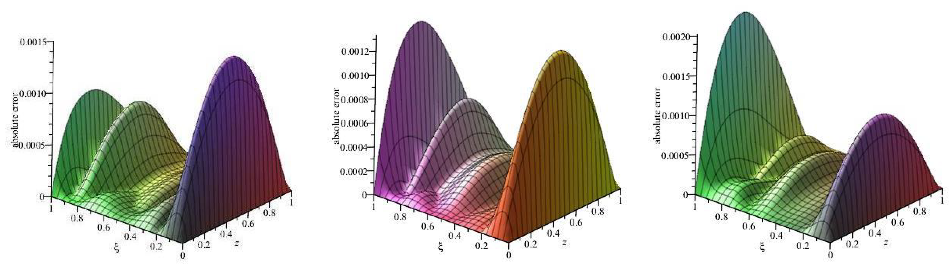
Example 1.
It will be examined that the following fractional-order Burgers’ problem with Dirichlet boundary condition:
c D ξ α u + ( 1 + z ξ ) u z z + z 2 u + ( z + 1 ) u z ξ sin ( z ) u u z = f ( z , ξ )
0 ξ 1 , 0 z 1 , 0 < α 1 ,
u ( z , 0 ) = 0 = u ( 0 , ξ ) = u ( 1 , ξ ) = 0 .
The exact solution of problem:
u ( z , ξ ) = ( z 2 z ) ξ 1 + α ,
and f ( z , ξ ) is the function that provides the Equation (62). Taking z i = i a , i = 1 , 2 , . . . , a , ξ i = i b , i = 1 , 2 , . . . , b and n-th term of approximate solution is selected as n = a × b . Absolute error values for Example 1 is computed for α = 0.9 , α = 0.8 , α = 0.7 and n = 25 ( a = b = 5 ) . Error values are given in Table 2, Table 3 and Table 4 in order to observe of applicability and influence of method. The graphics of absolute errors are given for α = 0.7 , α = 0.8 , and α = 0.9 in Figure 1.
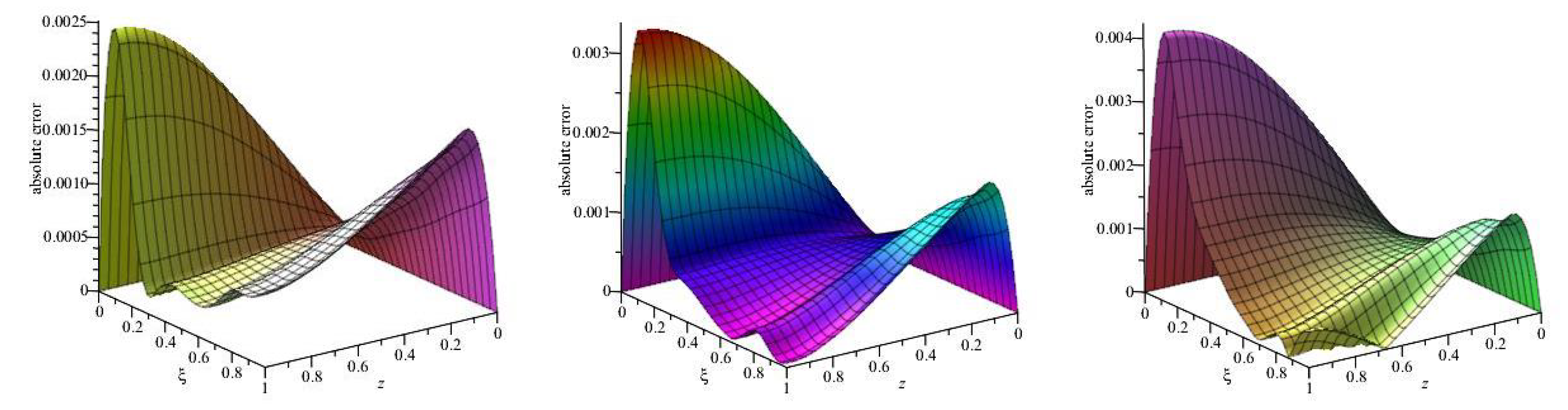
Example 2.
It will be examined that the fractional-order Burgers’ equation with Neumann boundary condition as follow:
c D ξ α u u z z u u z = f ( z , ξ )
0 z 1 , 0 ξ 1 , 1 2 < α 1 ,
u ( z , 0 ) = 0 , u z ( 0 , ξ ) = u z ( 1 , ξ ) = 0 .
The exact solution of problem is:
u ( z , ξ ) = ( z 3 3 z 2 2 ) ξ 2 α ,
and f ( z , ξ ) is the function that provides the Equations (65). Taking z i = i a , i = 1 , 2 , . . . , a , ξ i = i b , i = 1 , 2 , . . . , b and n = a × b . Absolute error of Example 2 is computed for α = 0.9 , α = 0.8 , α = 0.7 and n = 64 ( a = b = 8 ) . Error values are given in Table 5, Table 6 and Table 7 in order to observe of applicability and influence of method. The graphics of absolute errors are given for α = 0.7 , α = 0.8 , and α = 0.9 in Figure 2.

7. Conclusions

In this research, some special Hilbert spaces with inner products and the kernel function of these spaces are introduced. Then the iterative solution is obtained by reproducing kernel theory. Error estimation of the approximate solution and convergence analysis are verified with lemma and theorems. Numerical outcomes demonstrate that the iterative approximation is applicable, convenient, and powerful for fractional-order Burgers’ equation with Dirichlet and Neumann conditions. Therefore, iterative RKM is successfully implemented for fractional-order Burgers’ equation and so this study will contribute to the science.

Author Contributions

Resources, F.E.; Software, M.G.S.; Writing-original draft, O.S.; Writing-review & editing, O.S. and M.G.S. All authors have read and agreed to the published version of the manuscript.

Funding

This research received no funding.

Acknowledgments

We thank the reviewers for their positive remarks on our work.

Conflicts of Interest

The authors declare no conflict of interest.

Abbreviations

The following abbreviations are used in this manuscript:
RKMReproducing Kernel Method
RKHSReproducing Kernel Hilbert Space

References

  1. Burgers, J.M. Mathematical examples illustrating relations occurring in the theory of turbulent fluid motion. In Selected Papers of JM Burgers; Verhandelingen Der Koninklijke Nederlandsche Akademle V An Wetenschappen, Afdeeling Natuurkunde; Springer: Dordrecht, The Netherlands, 1939; Volume 17, pp. 1–53. [Google Scholar]
  2. Guesmia, A.; Daili, N. About the existence and uniqueness of solution to fractional Burgers Equation. Acta Univ. Apulensis 2010, 21, 161–170. [Google Scholar]
  3. Lombard, B.; Matignon, D. Diffusive approximation of a time-fractional Burger’s equation in nonlinear acoustics. Siam J. Appl. Math. 2016, 76, 1765–1791. [Google Scholar] [CrossRef] [Green Version]
  4. Dong, Z.; Sun, X.; Xiao, H.; Zhai, J. Averaging principle for one dimensional stochastic Burgers equation. J. Differ. Equ. 2018, 265, 4749–4797. [Google Scholar] [CrossRef] [Green Version]
  5. Nojavan, H.; Abbasbandy, S.; Mohammadi, M. Local variably scaled Newton basis functions collocation method for solving Burgers’ equation. Appl. Math. Comput. 2018, 330, 23–41. [Google Scholar] [CrossRef]
  6. Oruc, O.; Esen, A.; Bulut, F. A unified finite difference Chebyshev wavelet method for numerically solving time fractional Burgers’ equation. Discret. Contin. Dyn. Syst. Ser. S 2019, 12, 533–542. [Google Scholar]
  7. Rong-Pei, Z.; Xi-Jun, Y.; Guo-Zhong, Z. Modified Burgers’ equation by the local discontinuous Galerkin method. Chin. Phys. B 2013, 22, 1–5. [Google Scholar]
  8. Roshan, T.; Bhamra, K.S. Numerical solutions of the modified Burgers’ equation by Petrov-Galerkin method. Appl. Math. Comput. 2011, 218, 3673–3679. [Google Scholar] [CrossRef]
  9. Ramadan, M.A.; Danaf, T.S.E. Numerical treatment for the modified Burgers equation. Math. Comput. Simul. 2005, 70, 90–98. [Google Scholar] [CrossRef]
  10. Bahadir, A.R.; Saglam, M. A mixed finite difference and boundary element approach to one-dimensional Burgers’ equation. Appl. Math. Comput. 2005, 160, 663–673. [Google Scholar] [CrossRef]
  11. Dag, I.; Irk, D.; Saka, B. A numerical solution of the Burgers equation using cubic B-splines. Appl. Math. Comput. 2005, 163, 199–211. [Google Scholar]
  12. Caldwell, J.; Wanless, P.; Cook, E. A finite element approach to Burgers’ equation. Appl. Math. Model. 1981, 5, 189–193. [Google Scholar] [CrossRef] [Green Version]
  13. Kutluay, S.; Bahadir, A.R.; Ozdes, A. Numerical solution of one-dimensional Burgers’ equation: Explicit and exact-explicit finite-difference methods. J. Comput. Appl. 1999, 103, 251–261. [Google Scholar] [CrossRef] [Green Version]
  14. Li, F.; Cui, M. A best approximation for the solution of one-dimensional variable-coefficient Burgers equation. Numer. Methods Partial Differ. Equ. 2009, 25, 1353–1365. [Google Scholar] [CrossRef]
  15. Raza, N.; Awan, A.U.; Haque, E.U.; Abdullah, M.; Rashidi, M.M. Unsteady flow of a Burgers’ fluid with Caputo fractional derivatives: A hybrid technique. Ain Shams Eng. J. 2019, 10, 319–325. [Google Scholar] [CrossRef]
  16. Safdar, R.; Imran, M.; Khalique, C.M. Time-dependent flow model of a generalized Burgers’ fluid with fractional derivatives through a cylindrical domain: An exact and numerical approach. Results Phys. 2018, 9, 237–245. [Google Scholar] [CrossRef]
  17. Liu, J.; Hou, G. Numerical solutions of the space-and time-fractional coupled Burgers equations by generalized differential transform method. Appl. Math. Comput. 2011, 217, 7001–7008. [Google Scholar] [CrossRef]
  18. Zhang, J.; Liu, F.; Lin, Z.; Anh, V. Analytical and numerical solutions of a multi-term time-fractional Burgers’ fluid model. Appl. Math. Comput. 2019, 356, 1–12. [Google Scholar] [CrossRef]
  19. Momani, S. Non-perturbative analytical solutions of the space-and time-fractional Burgers equations. Chaos Solitons Fractals 2006, 28, 930–937. [Google Scholar] [CrossRef]
  20. Ajou, A.E.; Arqub, O.A.; Momani, S. Approximate analytical solution of the nonlinear fractional KdV-Burgers equation: A new iterative algorithm. J. Comput. Phys. 2015, 293, 81–95. [Google Scholar] [CrossRef]
  21. Mittal, R.C.; Arora, G. Numerical solution of the coupled viscous Burgers’ equation. Commun. Nonlinear. Sci. Numer. Simulat. 2011, 16, 1304–1313. [Google Scholar] [CrossRef]
  22. Jiwari, R. A hybrid numerical scheme for the numerical solution of the Burgers’ equation. Comput. Phys. Commun. 2015, 188, 59–67. [Google Scholar] [CrossRef]
  23. Kutluay, S.; Esen, A.; Dag, I. Numerical solutions of the Burgers’ equation by the least-squares quadratic B-spline finite element method. J. Comput. Appl. Math. 2004, 167, 21–33. [Google Scholar] [CrossRef] [Green Version]
  24. Zaremba, S. Sur le calcul numérique des fonctions demandées dans le probléme de Dirichlet et le problème hydrodynamique. Bull. Int. de l’Académie Sci. Cracovie 1908, 1908, 125–195. [Google Scholar]
  25. Aronszajn, N. Theory of reproducing kernels. Trans. Am. Math. Soc. 1950, 68, 337–404. [Google Scholar] [CrossRef]
  26. Schwartz, L. Sous-espaces hilbertiens d’espaces vectoriels topologiques et noyaux associés (noyaux reproduisants). J. Anal. Math. 1964, 13, 115–256. [Google Scholar] [CrossRef]
  27. Saitoh, S.; Sawano, Y. Theory of Reproducing Kernels and Applications. Developments in Mathematics; Springer: Singapore, 2016. [Google Scholar]
  28. Akram, G.; Rehman, H. Numerical solution of eighth order boundary value problems in reproducing Kernel space. Numer. Algor. 2013, 62, 527–540. [Google Scholar] [CrossRef]
  29. Jiang, W.; Lin, Y. Approximate solution of the fractional advection-dispersion equation. Comput. Phys. Commun. 2010, 181, 557–561. [Google Scholar] [CrossRef]
  30. Arqub, O.A. Numerical algorithm for the solutions of fractional order systems of Dirichlet function types with comparative analysis. Fundam. Inform. 2019, 166, 111–137. [Google Scholar] [CrossRef]
  31. Sakar, M.G.; Saldır, O.; Akgül, A. A novel technique for fractional Bagley–Torvik equation. Proc. Natl. Acad. Sci. India Sect. A Phys. Sci. 2019, 89, 539–545. [Google Scholar] [CrossRef]
  32. Jiang, W.; Lin, Y. Representation of exact solution for the time-fractional telegraph equation in the reproducing kernel space. Commun. Nonlinear Sci. Numer. Simulat. 2011, 16, 3639–3645. [Google Scholar] [CrossRef]
  33. Mohammadi, M.; Zafarghandi, F.S.; Babolian, E.; Jvadi, S. A local reproducing kernel method accompanied by some different edge improvement techniques: Application to the Burgers’ equation. Iran. J. Sci. Technol. Trans. Sci. 2018, 42, 857–871. [Google Scholar] [CrossRef]
  34. Arqub, O.A.; Al-Smadi, M. Numerical algorithm for solving time-fractional partial integrodifferential equations subject to initial and Dirichlet boundary conditions. Numer. Methods Partial Differ. Equ. 2018, 34, 1577–1597. [Google Scholar] [CrossRef]
  35. Sakar, M.G. Iterative reproducing kernel Hilbert spaces method for Riccati differential equations. J. Comput. Appl. Math. 2017, 309, 163–174. [Google Scholar] [CrossRef]
  36. Yao, H. Reproducing Kernel method for the solution of nonlinear hyperbolic telegraph equation with an integral condition. Numer. Methods Partial Differ. Equ. 2011, 27, 867–886. [Google Scholar] [CrossRef]
  37. Arqub, O.A. Solutions of time-fractional Tricomi and Keldysh equations of Dirichlet functions types in Hilbert space. Numer. Methods Partial Differ. Equ. 2018, 34, 1759–1780. [Google Scholar] [CrossRef]
  38. Akgül, A.; Inc, M.; Kilicman, A.; Baleanu, D. A new approach for one-dimensional sine-Gordon equation. Adv. Differ. Equ. 2010, 8, 1–20. [Google Scholar] [CrossRef] [Green Version]
  39. Lin, Y.; Zhou, Y. Solving the reaction-diffusion equations with nonlocal boundary conditions based on reproducing kernel space. Numer. Methods Partial Differ. Equ. 2009, 25, 1468–1481. [Google Scholar] [CrossRef]
  40. Arqub, O.A.; Maayah, B. Numerical solutions of integro differential equations of Fredholm operator type in the sense of the Atangana-Baleanu fractional operator. Chaos Solitons Fractals 2018, 117, 117–124. [Google Scholar] [CrossRef]
  41. Arqub, O.A.; Al-Smadi, M.; Shawagfeh, N. Solving Fredholm integro-differentialequations using reproducing kernel Hilbert space method. Appl. Math. Comput. 2013, 219, 8938–8948. [Google Scholar]
  42. Mohammadi, M.; Mokhtari, R. A reproducing kernel method for solving a class of nonlinear systems of PDEs. Math. Model. Anal. 2014, 19, 180–198. [Google Scholar] [CrossRef]
  43. Wang, Y.; Du, M.; Tan, F.; Li, Z.; Nie, T. Using reproducing kernel for solving a class of fractional partial differential equation with non-classical conditions. Appl. Math. Comput. 2013, 219, 5918–5925. [Google Scholar] [CrossRef]
  44. Arqub, O.A.; Al-Smadi, M. Atangana-Baleanu fractional approach to the solutions of Bagley–Torvik and Painlevéequations in Hilbert space. Chaos Solitons Fractals 2018, 117, 161–167. [Google Scholar] [CrossRef]
  45. Mohammadi, M.; Mokhtari, R.; Panahipour, H. A Galerkin-reproducing kernel method: Application to the 2D nonlinear coupled Burgers equations. Eng. Anal. Bound. Elem. 2013, 37, 1642–1652. [Google Scholar] [CrossRef]
  46. Sakar, M.G.; Saldır, O. Improving variational iteration method with auxiliary parameter for nonlinear time-fractional partial differential equations. J. Optim. Theory Appl. 2017, 174, 530–549. [Google Scholar] [CrossRef]
  47. Cui, M.G.; Lin, Y.Z. Nonlinear Numercal Analysis in the Reproducing Kernel Space; Nova Science Publisher: New York, NY, USA, 2009. [Google Scholar]
  48. Tanaka, K. Generation of point sets by convex optimization for interpolation in reproducing kernel Hilbert spaces. Numer. Algor. 2019, 84, 1049–1079. [Google Scholar] [CrossRef] [Green Version]
  49. Sakar, M.G.; Saldır, O.; Erdogan, F. An iterative approximation for time-fractional Cahn-Allen equation with reproducing kernel method. Comput. Appl. Math. 2018, 37, 5951–5964. [Google Scholar] [CrossRef]
  50. Lotfi, T.; Rashidi, M.; Mahdiani, K. A posteriori analysis: Error estimation for the eighth order boundary value problems in reproducing Kernel space. Numer. Algor. 2016, 73, 391–406. [Google Scholar] [CrossRef]
  51. Saldır, O.; Sakar, M.G.; Erdogan, F. Numerical solution of time-fractional Kawahara equation using reproducing kernel method with error estimate. Comp. Appl. Math. 2019, 38, 198. [Google Scholar] [CrossRef]
  52. Bakhtiari, P.; Abbasbandy, S.; Van Gorder, R.A. Solving the Dym initial value problem in reproducing kernel space. Numer. Algor. 2018, 78, 405–421. [Google Scholar] [CrossRef]
  53. Sakar, M.G.; Saldır, O.; Erdogan, F. A hybrid method for singularly perturbed convection–diffusion equation. Int. J. Appl. Comput. Math. 2019, 5, 135. [Google Scholar] [CrossRef]
  54. Sakar, M.G.; Saldır, O. A novel iterative solution for time-fractional Boussinesq equation by reproducing kernel method. J. Appl. Math. Comput. 2020, in press. [Google Scholar] [CrossRef]
  55. Gao, W.; Veeresha, P.; Prakasha, D.G.; Baskonus, H.M. Novel Dynamic Structures of 2019-nCoV with Nonlocal Operator via Powerful Computational Technique. Biology 2020, 9, 107. [Google Scholar] [CrossRef] [PubMed]
  56. Goufo, E.F.D.; Toudjeo, I.T. Around chaotic disturbance and irregularity for higher order traveling waves. J. Math. 2018, 2018, 2391697. [Google Scholar]
  57. Goufo, E.F.D. Application of the Caputo-Fabrizio fractional derivative without singular kernel to Korteweg-de Vries-Burgers equation. Math. Model. Anal. 2016, 21, 188–198. [Google Scholar] [CrossRef]
  58. Podlubny, I. Fractional Differential Equations; Academic Press: New York, NY, USA, 1999. [Google Scholar]
  59. Diethelm, K. The Analysis of Fractional Differential Equations; Lecture Notes in Mathematics; Springer: Berlin/Heidelberg, Germany, 2010. [Google Scholar]
Figure 1. The surfaces show the absolute error of Example 1 with n = 16 ( a = b = 4 ) and for α = 0.7 , α = 0.8 , α = 0.9 respectively on region Θ .
Fractalfract 04 00027 g001
Figure 2. The surfaces show the absolute error of Example 2 with n = 36 ( a = b = 6 ) and for α = 0.7 , α = 0.8 , α = 0.9 respectively on region Θ .
Fractalfract 04 00027 g002
Table 1. Notation table.
SymbolExplanation
c D ξ α Caputo derivative operator with arbitrary real order
Θ Region of [ 0 , 1 ] × [ 0 , 1 ]
W 2 3 [ 0 , 1 ] Hilbert space with one variable function
W 2 ( 3 , 2 ) ( Θ ) Hilbert Space with two variable function
K ( τ , β ) ( z , ξ ) Reproducing kernel function of W 2 ( 3 , 2 ) ( Θ )
u ( z , ξ ) Exact solution
u n ( z , ξ ) Reproducing kernel solution
LLinear operator
. , . Inner (scalar) product
Table 2. Absolute error values of Example 1 for Burgers’ equation with α = 0.9 .
z / ξ 0.1 0.2 0.3 0.4 0.5 0.6 0.7 0.8 0.9
0.1 1.31 × 10 4 3.13 × 10 5 3.36 × 10 5 3.90 × 10 5 5.67 × 10 5 5.06 × 10 5 6.67 × 10 5 2.92 × 10 5 1.31 × 10 4
0.2 2.34 × 10 4 5.74 × 10 5 6.39 × 10 5 7.70 × 10 5 1.13 × 10 4 1.08 × 10 4 1.44 × 10 4 1.55 × 10 5 1.83 × 10 4
0.3 3.07 × 10 4 7.60 × 10 5 8.59 × 10 5 1.05 × 10 4 1.55 × 10 4 1.53 × 10 4 2.07 × 10 4 7.90 × 10 6 1.96 × 10 4
0.4 3.49 × 10 4 8.65 × 10 5 9.88 × 10 5 1.22 × 10 4 1.82 × 10 4 1.81 × 10 4 2.51 × 10 4 3.54 × 10 5 1.75 × 10 4
0.5 3.62 × 10 4 8.76 × 10 5 1.00 × 10 4 1.24 × 10 4 1.87 × 10 4 1.88 × 10 4 2.66 × 10 4 5.70 × 10 5 1.33 × 10 4
0.6 3.45 × 10 4 8.13 × 10 5 9.31 × 10 5 1.16 × 10 4 1.75 × 10 4 1.76 × 10 4 2.57 × 10 4 7.18 × 10 5 7.86 × 10 5
0.7 2.99 × 10 4 6.69 × 10 5 7.60 × 10 5 9.49 × 10 5 1.45 × 10 4 1.44 × 10 4 2.19 × 10 4 7.05 × 10 5 3.03 × 10 5
0.8 2.25 × 10 4 4.73 × 10 5 5.30 × 10 5 6.56 × 10 5 1.01 × 10 4 9.98 × 10 5 1.58 × 10 4 5.56 × 10 5 3.62 × 10 6
0.9 1.25 × 10 4 2.41 × 10 5 2.63 × 10 5 3.22 × 10 5 5.09 × 10 5 4.82 × 10 5 8.20 × 10 5 2.96 × 10 5 1.49 × 10 5
Table 3. Absolute error values of Example 1 for Burgers’ equation with α = 0.8 .
z / ξ 0.1 0.2 0.3 0.4 0.5 0.6 0.7 0.8 0.9
0.1 1.26 × 10 4 1.29 × 10 5 2.37 × 10 5 1.99 × 10 5 4.07 × 10 5 3.53 × 10 5 6.82 × 10 5 1.27 × 10 5 8.96 × 10 6
0.2 2.25 × 10 4 2.58 × 10 5 4.78 × 10 5 4.48 × 10 5 8.67 × 10 5 8.28 × 10 5 1.48 × 10 4 5.90 × 10 5 3.22 × 10 5
0.3 2.96 × 10 4 3.61 × 10 5 6.66 × 10 5 6.49 × 10 5 1.23 × 10 4 1.21 × 10 4 2.13 × 10 4 1.03 × 10 4 8.09 × 10 5
0.4 3.39 × 10 4 4.36 × 10 5 7.94 × 10 5 7.88 × 10 5 1.47 × 10 4 1.48 × 10 4 2.57 × 10 4 1.40 × 10 4 1.30 × 10 4
0.5 3.53 × 10 4 4.62 × 10 5 8.30 × 10 5 8.22 × 10 5 1.54 × 10 4 1.55 × 10 4 2.72 × 10 4 1.58 × 10 4 1.67 × 10 4
0.6 3.39 × 10 4 4.54 × 10 5 7.99 × 10 5 7.82 × 10 5 1.46 × 10 4 1.47 × 10 4 2.61 × 10 4 1.60 × 10 4 1.89 × 10 4
0.7 2.96 × 10 4 3.94 × 10 5 6.77 × 10 5 6.43 × 10 5 1.22 × 10 4 1.20 × 10 4 2.21 × 10 4 1.39 × 10 4 1.85 × 10 4
0.8 2.25 × 10 4 2.95 × 10 5 4.93 × 10 5 4.46 × 10 5 8.69 × 10 5 8.34 × 10 5 1.59 × 10 4 1.01 × 10 4 1.52 × 10 4
0.9 1.26 × 10 4 1.60 × 10 5 2.59 × 10 5 2.17 × 10 5 4.40 × 10 5 4.03 × 10 5 8.22 × 10 5 5.19 × 10 5 8.97 × 10 5
Table 4. Absolute error values of Example 1 for Burgers’ equation with α = 0.7 .
z / ξ 0.1 0.2 0.3 0.4 0.5 0.6 0.7 0.8 0.9
0.1 1.29 × 10 4 7.61 × 10 6 2.09 × 10 5 9.72 × 10 6 3.07 × 10 5 2.01 × 10 5 4.75 × 10 5 1.57 × 10 5 4.67 × 10 5
0.2 2.30 × 10 4 9.60 × 10 6 4.42 × 10 5 2.82 × 10 5 7.08 × 10 5 5.80 × 10 5 1.13 × 10 4 6.51 × 10 5 1.30 × 10 4
0.3 3.03 × 10 4 8.97 × 10 6 6.33 × 10 5 4.46 × 10 5 1.04 × 10 4 9.12 × 10 5 1.69 × 10 4 1.11 × 10 4 2.07 × 10 4
0.4 3.48 × 10 4 5.73 × 10 6 7.73 × 10 5 5.69 × 10 5 1.27 × 10 4 1.15 × 10 4 2.08 × 10 4 1.48 × 10 4 2.68 × 10 4
0.5 3.64 × 10 4 2.22 × 10 6 8.27 × 10 5 6.07 × 10 5 1.35 × 10 4 1.24 × 10 4 2.23 × 10 4 1.64 × 10 4 3.03 × 10 4
0.6 3.53 × 10 4 2.36 × 10 6 8.15 × 10 5 5.87 × 10 5 1.30 × 10 4 1.20 × 10 4 2.16 × 10 4 1.64 × 10 4 3.09 × 10 4
0.7 3.11 × 10 4 5.08 × 10 6 7.10 × 10 5 4.82 × 10 5 1.10 × 10 4 1.00 × 10 4 1.84 × 10 4 1.40 × 10 4 2.80 × 10 4
0.8 2.39 × 10 4 6.20 × 10 6 5.32 × 10 5 3.31 × 10 5 7.91 × 10 5 7.04 × 10 5 1.33 × 10 4 1.01 × 10 4 2.17 × 10 4
0.9 1.35 × 10 4 4.68 × 10 6 2.90 × 10 5 1.57 × 10 5 4.05 × 10 5 3.47 × 10 5 6.90 × 10 5 5.18 × 10 5 1.22 × 10 4
Table 5. Absolute error values of Example 2 for Burgers’ equation with α = 0.9 .
z / ξ 0.1 0.2 0.3 0.4 0.5 0.6 0.7 0.8 0.9
0.1 4.76 × 10 4 3.40 × 10 4 2.88 × 10 4 2.92 × 10 4 3.24 × 10 4 3.84 × 10 4 4.64 × 10 4 5.77 × 10 4 6.89 × 10 4
0.2 9.30 × 10 4 6.16 × 10 4 4.62 × 10 4 4.00 × 10 4 3.81 × 10 4 4.03 × 10 4 4.50 × 10 4 5.49 × 10 4 6.38 × 10 4
0.3 1.36 × 10 3 8.71 × 10 4 6.16 × 10 4 4.88 × 10 4 4.16 × 10 4 3.97 × 10 4 4.09 × 10 4 4.88 × 10 4 5.54 × 10 4
0.4 1.77 × 10 3 1.10 × 10 3 7.50 × 10 4 5.58 × 10 4 4.33 × 10 4 3.72 × 10 4 3.48 × 10 4 4.06 × 10 4 4.49 × 10 4
0.5 2.15 × 10 3 1.30 × 10 3 8.62 × 10 4 6.09 × 10 4 4.34 × 10 4 3.33 × 10 3 2.74 × 10 4 3.09 × 10 4 3.30 × 10 4
0.6 2.47 × 10 3 1.46 × 10 3 9.49 × 10 4 6.42 × 10 4 4.20 × 10 4 2.82 × 10 4 1.91 × 10 4 2.02 × 10 4 2.01 × 10 4
0.7 2.74 × 10 3 1.59 × 10 3 1.01 × 10 3 6.56 × 10 4 3.94 × 10 4 2.23 × 10 4 1.01 × 10 4 9.05 × 10 5 6.96 × 10 4
0.8 2.93 × 10 3 1.68 × 10 3 1.04 × 10 3 6.56 × 10 4 3.62 × 10 4 1.63 × 10 4 1.72 × 10 5 1.43 × 10 5 5.21 × 10 5
0.9 3.05 × 10 3 1.73 × 10 3 1.06 × 10 3 6.49 × 10 4 3.32 × 10 4 1.15 × 10 4 4.78 × 10 5 9.40 × 10 5 1.43 × 10 4
Table 6. Absolute error values of Example 2 for Burgers’ equation with α = 0.8 .
z / ξ 0.1 0.2 0.3 0.4 0.5 0.6 0.7 0.8 0.9
0.1 3.88 × 10 4 2.19 × 10 4 2.12 × 10 4 2.49 × 10 4 3.02 × 10 4 3.77 × 10 4 4.63 × 10 4 5.77 × 10 4 6.84 × 10 4
0.2 7.52 × 10 4 3.60 × 10 4 2.88 × 10 4 2.86 × 10 4 3.07 × 10 4 3.59 × 10 4 4.23 × 10 4 5.31 × 10 4 6.22 × 10 4
0.3 1.10 × 10 3 4.88 × 10 4 3.52 × 10 4 3.10 × 10 4 2.96 × 10 4 3.21 × 10 4 3.61 × 10 4 4.60 × 10 4 5.34 × 10 4
0.4 1.44 × 10 3 6.01 × 10 4 4.05 × 10 4 3.23 × 10 4 2.74 × 10 4 2.73 × 10 4 2.88 × 10 4 3.74 × 10 4 4.32 × 10 4
0.5 1.75 × 10 3 6.97 × 10 4 4.45 × 10 4 3.26 × 10 4 2.43 × 10 4 2.16 × 10 4 2.07 × 10 4 2.79 × 10 4 3.21 × 10 4
0.6 2.01 × 10 3 7.75 × 10 4 4.74 × 10 4 3.19 × 10 4 2.05 × 10 4 1.53 × 10 4 1.22 × 10 4 1.79 × 10 4 2.06 × 10 4
0.7 2.23 × 10 3 8.31 × 10 4 4.90 × 10 4 3.04 × 10 4 1.62 × 10 4 8.89 × 10 5 3.63 × 10 5 7.85 × 10 5 9.18 × 10 5
0.8 2.40 × 10 3 8.68 × 10 4 4.95 × 10 4 2.85 × 10 4 1.20 × 10 4 2.81 × 10 5 4.19 × 10 5 1.33 × 10 5 1.18 × 10 5
0.9 2.50 × 10 3 8.87 × 10 4 4.94 × 10 4 2.67 × 10 4 8.76 × 10 5 1.80 × 10 5 1.00 × 10 4 8.19 × 10 5 8.88 × 10 4
Table 7. Absolute error values of Example 2 for Burgers’ equation with α = 0.7 .
z / ξ 0.1 0.2 0.3 0.4 0.5 0.6 0.7 0.8 0.9
0.1 2.86 × 10 4 1.42 × 10 4 1.89 × 10 4 2.48 × 10 4 3.17 × 10 4 4.00 × 10 4 4.88 × 10 4 5.96 × 10 4 6.96 × 10 4
0.2 5.41 × 10 4 1.88 × 10 4 2.15 × 10 4 2.53 × 10 4 3.01 × 10 4 3.73 × 10 4 4.48 × 10 4 5.53 × 10 4 6.41 × 10 4
0.3 7.93 × 10 4 2.26 × 10 4 2.34 × 10 4 2.50 × 10 4 2.77 × 10 4 3.35 × 10 4 3.95 × 10 4 4.95 × 10 4 5.71 × 10 4
0.4 1.03 × 10 3 2.57 × 10 4 2.49 × 10 4 2.42 × 10 4 2.48 × 10 4 2.91 × 10 4 3.36 × 10 4 4.30 × 10 4 4.95 × 10 4
0.5 1.26 × 10 3 2.81 × 10 4 2.58 × 10 4 2.30 × 10 4 2.16 × 10 4 2.45 × 10 4 2.75 × 10 4 3.61 × 10 4 4.16 × 10 4
0.6 1.45 × 10 3 2.98 × 10 4 2.62 × 10 4 2.14 × 10 4 1.81 × 10 4 1.96 × 10 4 2.12 × 10 4 2.91 × 10 4 3.36 × 10 4
0.7 1.62 × 10 3 3.06 × 10 4 2.60 × 10 4 1.95 × 10 4 1.45 × 10 4 1.48 × 10 4 1.52 × 10 4 2.22 × 10 4 2.58 × 10 4
0.8 1.74 × 10 3 3.09 × 10 4 2.55 × 10 4 1.76 × 10 4 1.12 × 10 4 1.04 × 10 4 9.79 × 10 5 1.59 × 10 4 1.89 × 10 4
0.9 1.82 × 10 3 3.08 × 10 4 2.50 × 10 4 1.60 × 10 4 8.69 × 10 5 7.20 × 10 5 5.79 × 10 5 1.14 × 10 4 1.38 × 10 4

