1. Introduction
Without a doubt, complex analytic functions are both a rich and beautiful area of mathematical pursuit and one of the most powerful tools used in physics to gain insight into countless natural phenomena. One important reason for this is that singularities—the points where analyticity breaks down—carry physical information about the system. The most immediate example is the damped simple harmonic oscillator, where the position of the associated pole in the complex plane gives the natural frequency and damping constant. Analytic functions can be represented by Taylor series, the radius of convergence of which are restricted by singular points. For the ubiquitous case of functions having only isolated singularities, analytic continuation can be performed to expand the domain of the function throughout the complex plane (or, more generally, Riemann sheet).
A much less frequently explored class of analytic functions are those with singular curves called natural boundaries, which are impenetrable to analytic continuation [
1,
2]. Of particular note are the lacunary functions. These are functions that exhibit a natural boundary and whose power series has absent terms—“gaps” or “lacunae”—in the progression of the exponential powers within the expansion. One simple example is
, which has a natural boundary on the unit circle. The function is analytic in the open unit disk and cannot be analytically continued beyond the unit circle.
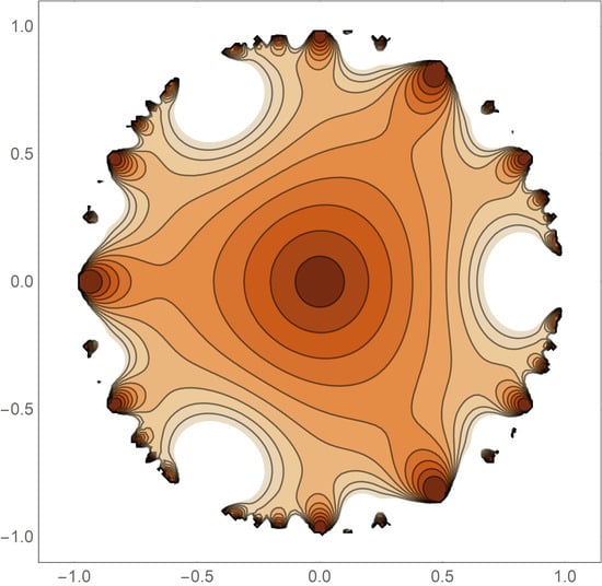
Figure 1 shows a graphical representation of the modulus of this function. The lower right panel representation, which shows a contour plot of
, is used throughout this work.
In general, Hadamard’s gap theorem establishes the criterion for the presence of a natural boundary of series with gaps [
2]. The lacunary functions explored in this work meet this criterion because the gaps in the exponential powers increase as the series expansion goes to infinity.
Due to analytic continuation not being possible through the natural boundary as well as additional complications, functions with natural boundaries have not often seen use in physics. Recently, however, lacunary functions have seen use in addressing physical problems. Natural boundaries influencing instanton orbiting was shown by Shudo and Ikeda to impact quantum tunneling [
3]. Creagh and White demonstrated the importance of natural boundaries in the short-wavelength approximation when calculating evanescent waves outside of elliptic dielectrics [
4]. Lacunary functions are related to Gauss sums, of which Schleich et al. discussed the many applications in physics [
5,
6]. Regarding integrable/nonintegrable systems, Greene and Percival worked with natural boundaries in their study of Hamiltonian maps [
7].
In statistical mechanics, Nickel proved that, within the calculation of the magnetic susceptibility in the 2D Ising model, there is the presence of a natural boundary [
8]. Additionally, several research groups have shown that any solution of an unsolvable Ising-like system must be able to be expressed in terms of functions having natural boundaries [
9,
10]. In kinetic theory, lacunary functions, upon approaching the natural boundary, have features that are closely tied to Weiner (stochastic) processes. Because of this, lacunary functions have been discussed in the context of Brownian motion [
2,
11]. In quantum mechanics, Yamada and Ikeda examined the wavefunctions related to Anderson-localized states in the Harper model [
12].
Alongside physics, lacunary functions have found use in probability theory. Particular lacunary trigonometric systems [
13,
14] work as independent random variables. Criteria for the behavior of the gaps in order for these lacunary functions to be consistent with the central limit theorem have been established by several researchers [
13,
15,
16,
17]. Lacunary trigonometric systems are also of interest in the study of harmonic analysis on compact groups [
18,
19]. Costin and Huang provided a detailed study of the behavior of lacunary series at the natural boundary [
20]. Very recently, Boyd investigated the breakdown of the Darboux principle at the natural boundary of lacunary function [
21]. Dahlqvist studied conditions of the zeta function that produce natural boundaries [
22]. Additionally, lacunary functions are useful in partitioning theory [
23,
24,
25,
26]. Further, lacunary series have been discussed with their relationship to theta, mock theta, and Dedekind eta functions [
27,
28]. Tangentially related to the current work is the very recent study of Bohr’s inequality via lacunary series by Kayumov and Ponnusamy [
29] and Liu and Liu [
30]. Eckstein and Zaja̧c studied heat traces of unbounded operators in Hilbert space [
31]. In their investigation of Sobolev–Jacobo polynomials, Behr et.al. studied lacunary generation functions [
32]. Kişi, Gümüş, and Savas investigated
-lacunary convergence and Cesàro summability with respect to lacunary sequences [
33].
Recent work of the current authors has focused on centered polygonal lacunary functions [
34,
35,
36,
37]. The exponential power gaps for these functions are given by the centered polygonal numbers [
38,
39]. The modulus of centered polygonal lacunary functions exhibits rotational symmetry under a phase shift in the complex plane. This is related to the fact that lacunary functions also exhibit well organized behavior at the natural boundary [
34]. Most lacunary functions exhibit what is called quasi-symmetry [
34] but not true rotational symmetry. They also have fractal character [
36]. Insight from the study has allowed for an understanding of what must be true of the gap behavior in order for the lacunary function to exhibit true rotational symmetry as well as dihedral mirror symmetry. These symmetries are the topic of this work and the subject of four theorems presented below. Several examples are presented as is a discussion of the nature of the gap behavior and its effect on the form of the lacunary functions.
A second aspect of this paper is to develop two distinct renormalized products of centered polygonal lacunary functions which carry with them the rotational and dihedral mirror symmetry of the centered polygonal lacunary functions. The first renormalized product is simply a power of a single centered polygonal lacunary function. The second is a product of symmetry-related centered polygonal lacunary functions.
2. Definitions and Notation
The
Nth member of a lacunary sequence of functions is given by
where the function
satisfies Hadamard’s gap theorem [
2]. Note that the sum starts at
rather than at
[
34]. Further, to limit the scope of this work, only the cases where
and unit coefficients are considered. For convenience, Haramard’s theorem is repeated here as given in [
2].
Theorem 1. Hadamard’s Gap Theorem.
The analytic function defined by has a natural boundary on the boundary of its radius of convergence if there exists a fixed such that, for all n For most of what follows. is some sort of quadratic function. Consider the prototypical example of . In this case, for all n so there exists a fixed such that .
For convenience of notation. one defines
to represent the particular lacunary sequence described by
. The condensed notation,
, is used throughout to represent the
Nth member of
. The lacunary function associated with the sequence is defined in the limit,
The example from
Section 1 would be
and the specific function shown in
Figure 1 is
. Finally, it is noted that there are
N terms in the summations and that the sum truncates after the
th power, thus for
the highest power in the sum is
.
As a matter of convenience for the reader, several definitions and theorems regarding rotational symmetry are collected here. Proofs and other discussion can be found in [
34].
Definition 1. Centered polygonal number. The formula for the set of centered k-gonal numbers is Centered polygonal numbers are an infinite, increasing sequence of numbers associated with points on a polygonal lattice [
38,
39,
40,
41]. Teo and Sloane [
39] discussed centered polygonal numbers in the context of two-dimensional crystal structures. The centered polygonal numbers are related to the more familiar polygonal numbers,
[
40,
41]. Note
are the ubiquitous triangular numbers.
Lemma 1. .
Proof. The proof is given in [
34]. □
For the special case of triangular numbers,
Proof. The proof is given in [
34]. □
When it comes to the source for , centered polygonal numbers give rise to lacunary functions that exhibit true rotational symmetry along with dihedral mirror symmetry. The polygonal numbers do not.
Definition 2. Main unity contour. The simple closed rectifiable curve marking the boundary of the set of points, z, such that and are path-connected to the origin.
Definition 3. Primary symmetry. The rotational symmetry of the member of , , is called the primary symmetry.
Theorem 2. The primary symmetry of is .
Proof. The proof is given in [
34]. □
Corollary 1. The primary symmetry of the centered polygonal lacunary functions () is k, i.e., .
Proof. The proof is given in [
34]. □
Definition 4. Symmetry angle. Let the primary symmetry be s-fold. The first symmetry angle is , . The pth symmetry angle is , .
3. Rotational and Dihedral Symmetry of Centered Polygonal Lacunary Functions
Turning attention to the centered polygonal lacunary functions, one sees clear
k-fold rotational symmetry. The examples of
,
, and
are shown in
Figure 2 which have three-, five-, and seven-fold true rotational symmetry, respectively. In addition to the rotational symmetry,
k dihedral mirror planes of symmetry exist. These appear at multiples of
, as clearly seen in
Figure 2. The proof of the existence of these symmetries is straightforward. The following two theorems establish these symmetries. When considering centered polygonal lacunary functions,
is written as
to expose the
k parameter.
Theorem 3. The functions in the set have k-fold rotational symmetry at the modulus level, where k is any positive integer.
Proof. The complex variable
z is represented in polar form,
. Writing out the
Nth member of the lacunary sequence
, one has
Now, consider
,
Upon evaluating the modulus, . Hence, k-fold rotational symmetry is present and evident in the unity contour plots. □
Theorem 4. The functions in the set have dihedral mirror symmetry at the primary symmetry angles at the modulus level (see Figure 2). Proof. Recognizing
as
, one has
Now, consider the mirror reflection about the line at
,
Thus, is of the form and is of the form . These two expressions are equivalent under the modulus , thus proving the dihedral mirror symmetry at the modulus level. □
4. Constructing Rotationally Symmetric Lacunary Functions
The case of the centered polygonal lacunary functions provides insight into what must be true of the behavior of the gaps in the power series. In the above proofs, one notices the cancellation of the k for all the n-dependent phase factors. If this is true, then the lacuanary function will have true rotational symmetry and dihedral mirror symmetry at the modulus level.
This insight leads to a method to construct lacunary functions that exhibit rotational and dihedral mirror symmetry. The main idea is that
must be chosen as such to produce the same rotational symmetry as the primary symmetry. To aid in thinking, consider
, with
chosen as follows: Choose an
which gives rise to an infinite, strictly increasing, superlinear sequence such that the first two members of the series are 0 and 1, i.e.,
and
. This will yield a primary symmetry (and hence quasi-symmetry) of
, hence
. Further, the
n-dependent part of
is homogeneous and linear in
s. This will allow the
s to cancel out of the phase factors similar to in the proofs in
Section 3. The above conditions on
can be loosened such that it only matters that the first two values of the sequence generated by
differ by one. The more restricted version is used in this work to ensure the first power of
z is present in the power series.
The above ideas can be collected into general symmetry theorems as follows.
Theorem 5. Let s and n be positive integers. The members of have s-fold rotational symmetry at the modulus level when .
Proof. The proof follows that of Theorem 3. Writing out the
Nth member of the lacunary sequence
, one has
Now, consider
,
Thus, at the modulus level, . □
Notice that, although the scope of this work considers only the cases where and , Theorem 5 does not require that restriction. The dihedral mirror symmetry follows similarly.
Theorem 6. The members of have dihedral mirror symmetry along multiples of at the modulus level when .
Proof. Similar to how the proof of Theorem 5 follows that of Theorem 3, so does the proof of this theorem follow that of Theorem 4.
Since is real, , as it is for the similar case of Theorem 4. Thus, there exist dihedral mirror symmetry at . □
By way of concrete example, the Fibonacci numbers are first considered:
. At first glance, it looks like this is a good candidate for an interesting
. However, the presence of two consecutive 1s does not make
strictly increasing. The two consecutive 1s will result in a power series where the coefficient of the
term is 2, not 1 as required. The scope of this paper is for lacunary functions of the form of Equation (
1). (The generalization to non-unity coefficients is an important one and should be a fertile ground for future research.) For completeness, this function is plotted in
Figure 3 where it does have rotational and mirror symmetry.
To get the Fibonacci sequence into a form that fits within the scope of this work, one can consider
, Thus, the first two members of the sequence generated by
are 0 and 1 as required and the sequence is superlinear and strictly increasing. The resultant lacunary functions is shown in
Figure 3b,c. Both symmetries are clearly evident. It is interesting to note how different the main unity contour plot is when compared to the directly-used Fibonacci sequence.
Sequences given by powers give rise to qualitatively different lacunary functions than those arising from the Fibonacci sequences.
Figure 4 shows the lacunary functions generated when
,
, and
. These sequences “accelerate” faster than the Fibonacci sequence in that the early numbers following the first 0 and 1 are much larger for the powers. However, the Fibonacci sequence ultimately surpasses the powers. The most notable qualitative distinction between the Fibonacci-based and power-based lacunary functions is the fact that the set bounded by the main unity contour is nearly convex for the power-based lacunary functions but that certainly is not the case for the Fibonacci-based lacunary functions. The manner in which
behaves has a significant influence on the qualitative shape of the main unity contour.
A more systematic study of the effect of the rapidness of the increase of the gap can be made by defining a function
where
is the floor of
x. The “weight” parameter,
w, softens the rising values of the sequence generated by
. The associated lacunary functions for several values of
w are shown in
Figure 5. As
w increases, qualitative changes to the associated lacunary functions are seen. This is especially true for low values of
w. As
w increases, the qualitative shape of the associated lacunary function settles into a single form with changes occurring only very near the natural boundary. As the rate of increase of the gap goes down, so does the convexity of the domain contained in the main unity contour.
Comparing
Figure 5,
Figure 3, and
Figure 4, one sees that, for small
w, the main unity contour is qualitatively similar to that for the power-based lacunary functions (
Figure 4). Conversely, for large
w, there is qualitative similarity with the Fibonacci-based lacunary function (
Figure 3). Of course, in both cases, there are numerous differences as well (especially near the natural boundary). This points to the sensitivity of the lacunary functions to the behavior of
.
5. Renormalized Products of Centered Polygonal Lacunary Functions
Having studied the rotational and mirror symmetry of certain lacunary functions, attention is returned to centered polygonal lacunary functions and, specifically, to the behavior of their products. These products also exhibit the same symmetries at the modulus level. Additionally, the notion of convexity of the main unity contour discussed above is also at play with the products.
The triangular lacunary series of Ramanujan is [
24,
42],
where
represents the
jth triangular number, which is well-known in partition theory [
42]. The
m-fold product,
can be expressed as
where
is the number of representations of the integer
n by
m triangular numbers [
42].
The triangular lacunary function is given by Equation (
17) by generalizing
q to complex variable
z:
. The following theorem showa how the centered polygonal lacunary functions are related to
.
Theorem 7. For any positive integer k, Proof. Starting from the right hand side of the theorem and using Equation (
7), one sees
Shifting the dummy index
The last expression is the centered polygonal lacunary function which completes the proof. □
A natural thing to consider about the centered polygonal functions is the behavior of their multiplicative powers. Simply multiplying the functions by themselves
j times gives rise to a leading power in the lacunary series to be equal to
j. It is of interest to place the product on equal footing, in terms of the leading power in the summation, with the original function and with other multiplicative powers. Hence, it is natural to renormalize the multiplicative power by dividing by the appropriate power of
z such that the leading term in the lacunary series is to the first power.
Figure 6 shows the difference between a non-renormalized power and a renormalized power for the case of
. In general, the unity level set is more convex for the renormalized case than it is for the non-renormalized case. In both cases, the polished nature of
, as defined in [
34], persists upon taking powers of the centered polygonal lacunary functions. Invariably, product functions will have associated lacunary series in which the coefficients are not all unity. Consequently, that requirement is suspended for the product functions.
5.1. Renormalized Powers
The connection between the triangular numbers and the centered polygonal numbers allows one to utilize the efficiency of the generating functions of in study of centered polygonal lacunary functions. Here, this is used to develop a renormalized power function and a symmetry sequence function.
The renormalized power of a centered polygonal lacunary functions is defined as follows.
Definition 5. Renormalized power. Let j and k be positive integers. The renormalized jth power of iswhen is truncated at N, The following theorem is an immediate result of Theorem 7 and Definition 5.
Theorem 8. Let j and k be positive integers. Then, Proof. From Definition 5 and application of Theorem 7,
The final relation follows from the summation form of . □
A subtle aspect of Theorem 8 is that the coefficients are decoupled from the powers. This is a manifestation of the important property of the centered polygonal lacunary functions that many of their characteristics are independent of
k. The same is true here. One need only find the
and one has the whole family of
. The case of
is shown in
Figure 7. The top left panel shows the original function, whereas the remaining panels shows increasing
j values. This example is illustrative of the general property of increasing convexity of the unity level set with increasing
j. Further, the
k-fold symmetry is maintained as well as the relative polish (again, see [
34]) of the unity level sets.
5.2. Symmetry-Sequence Products
In addition to multiplicative powers, it is equally natural to simply multiply two different centered polygonal lacunary functions. This certainly can be done but it will, in general, break the
k-fold rotational symmetry. An exception to this is the special case when an increasing sequence of
k values are chosen such that each larger
k is a multiple of the the base
k value. For example, the product
is one of these special sequences. For these types of products, the
k-fold rotational symmetry is maintained. This particular function is shown in
Figure 8. An elaborate and rather beautiful unity level set is seen. The presence of the higher
k factors in the product are responsible for this. Strong convexity is seen at the angles
.
The higher rotational symmetry factors
give rise to more structure in the function.
Figure 9 shows the case of
and
M increasing by 1 from 1 to 6.
Definition 6. Renormalized symmetry-sequence product. The k-based renormalized symmetry-sequence product of iswhen is truncated at N, Proof. Beginning with Definition 6,
Now, using Theorem 7, the
can be written in terms of
as
Now, expressing the
in their summation form gives
Combined with the presence of the other factors, one gets powers of
, 1 through
M. Then, by rearranging as in Equation (
19) for each power 1 through
M and factoring in the external factor of
z, one gets the final result
and the proof is completed. □
As long as
, all possible
exponents will appear and the above summation can be written more succinctly as
albeit
is rather complicated. In fact,
where
is interpreted as one of the ordered integer partitions of
n.
6. Conclusions
One focus of this work is the rotationally symmetric lacunary functions. This work builds upon previous studies of centered polygonal lacunary functions [
34,
35,
36] by adding to the literature two theorems regarding symmetry of these functions. The proven theorems show rotational and dihedral mirror symmetry carried by the centered polygonal lacunary functions at the modulus level. Beyond this, the theorems provide a general framework for constructing other lacunary functions that exhibit the same symmetries. Two additional theorems are given in this regard. This analysis enables a better explorations of the effects of the gap behavior on the qualitative features of the associated lacunary functions. By way of example, Fibonacci-based and power-based lacunary functions are given. Additionally, a parameterized, superlinear function allows for a more systematic study of the effects of gap behavior on the shape of the main unity contour. Fast acceleration of the underlying sequence given by
gives low convexity while slow acceleration yields high convexity.
One of the general features of functions related to the lacunary functions studied in previous work is that of self-similarity and scale-invariance [
5,
6,
20,
34,
36]. It may be the case that the knowledge of how to construct rotationally symmetric lacunary functions can be another tool in renormalization procedures.
Another focus of this work is the study of the behavior two types of products of centered polygonal lacunary functions, and . These functions exhibit the same rotational and dihedral mirror symmetry as the base centered polygonal lacunary functions.
Some obvious areas for further study include generalizing Equation (
1) to include non-unity coefficients, considering some of the numerous known sequences in addition to the Fibonacci and centered polygonal sequences, and continuing to try to connect to applications in physics and engineering. Potential areas of application in physics are to the partition function of statistical mechanics, nonlinear phase chirp in optics, and iterative dynamical systems.


