Power Law Type Long Memory Behaviors Modeled with Distributed Time Delay Systems

Abstract

This paper studies a class of distributed time delay systems that exhibit power law type long memory behaviors. Such dynamical behaviors are present in multiple domains and it is therefore essential to have tools to model them. The literature is full of examples in which these behaviors are modeled by means of fractional models. However, several limitations of fractional models have recently been reported and other solutions must be found. In the literature, the analysis of distributed delay models and integro-differential equations in general is older than that of fractional models. In this paper, it is shown that particular delay distributions and conditions on the model coefficients make it possible to obtain power laws. The class of systems considered is then used to model the input-output behavior of a lithium-ion cell.

1. Introduction

Systems with long memory behaviors sometimes generate outputs whose power spectrum $X\left(\omega \right)$ exhibits power laws ($X\left(\omega \right)\approx K/{\omega }^{2\nu }$) when supplied by white noise. Numerous examples of this kind of behavior have been revealed in various domains:

• Electrochemistry through charge diffusion in batteries [1,2,3,4];
• Thermal conduction through the exact solution of the heat equation in a semi-infinite medium linking the heat rate to the surface temperature [5,6];
• Biology through complex dynamics in biological tissues [7];
• Mechanics through the dynamical properties of viscoelastic materials and in particular wave propagation problems in these materials [8];
• Acoustics through visco-thermal losses in wind instruments [9];
• Electrical distribution networks [10].

The fractional integrator operator that links an input $u\left(t\right)$ to an output $y\left(t\right)$ and defined in the Riemann–Liouville sense by the Equation [11]

$$y\left(t\right)={{\displaystyle \int }}_0^t\frac{1}{{\left(t-\tau \right)}^{\nu -1}}u\left(\tau \right)d\tau ={}_0{}^{\nu }I\left\{u\left(t\right)\right\},$$

(1)

also exhibits this kind of behavior as the modulus of the Fourier transform of this operator, denoted $\left|Y\left(j\omega \right)/U\left(j\omega \right)\right|$ is defined by $1/{\omega }^{\nu }$. That is why a fractional order pseudo-state space description was introduced to model this kind of behavior. In the commensurate case and in most of the studies found in the literature, this description is defined by:

$$\{\begin{array}{c}\frac{d^{\nu }}{d{t}^{\nu }}x\left(t\right)=Ax\left(t\right)+Bu\left(t\right)\\ y\left(t\right)=Cx\left(t\right)\end{array}$$

(2)

where $\frac{d^{\nu }}{d{t}^{\nu }}$ is a fractional differentiation operator (which is, in a certain sense, the inverse operator to the operator ${}_0{}^{\nu }I\left\{\right\}$). There are several definitions for $\frac{d^{\nu }}{d{t}^{\nu }}$ in the literature [11]—more than 30 are listed in [12]—that are not all equivalent in relation to initial conditions [13,14,15].

Even if this kind of model provides a good fitting of the input-output behavior of many systems, Description (2) has several drawbacks:

• The variable $x\left(t\right)$ that plays the role of the state does not have the properties of a state, which is why the name pseudo-state was introduced [13,14];
• The initial conditions are not well taken into account if the Caputo or the Riemann–Liouville definitions are used for the derivative of the pseudo-state; it is better to define the description with a fractional integration to take into account the model past [13,14,15,16,17];
• The use of fractional differentiation in the pseudo-state space description is not mandatory and only fractional integration is needed [16];
• This description memory is infinite and it exhibits infinitely slow and fast time constants (even if they are attenuated, they exist), which excludes the possibility of linking the pseudo-state variable to a physical variable [14,16];
• Exact observability cannot be reached as all the system past must be known to predict its future [18];
• The fractional integration given by Equation (1) involves a singular kernel [19,20]. As mentioned in [20], this leads to complications in the solution/simulation of the fractional order differential equations;
• In modeling, several mathematical and interpretation problems can invalidate the models obtained [21].

In recent decades, there has been a frantic “fractionalization” of concepts and methods dedicated to integer models. It therefore seemed necessary to better define the benefits and limits of fractional models. Over many years of research in the field of fractional models, I have largely participated in updating several of the drawbacks previously mentioned. Faced with the omnipresence of phenomena and systems that exhibit power law behaviors, I became convinced that it was necessary to better understand the physical origins of these phenomena and it is proposed here to use other ways of modeling them than fractional models.

Thus, to overcome these problems and to model power law type long memory behavior, a class of distributed time delay models will be used here. Distributed time delay models, also known in the literature as hereditary models [22] or integro-differential equation-based models [23], have long existed. In this study, the delay distribution used in their definition is particularized in order to obtain the desired power law behaviors. The class of model considered is then applied to the modeling of a lithium-ion cell input-output behavior.

2. A Class of Time Delay Systems That Exhibits a Power Law Long Memory Behavior

The following class of distributed time delay systems is considered.

$$\begin{array}{c}\frac{d}{dt}x\left(t\right)=A_{0}x\left(t\right)+A_1{{\displaystyle \int }}_0^{T_f}\eta \left(\tau \right)x\left(t-\tau \right)d\tau +Bu\left(t\right)\\ \mathrm{with}{A}_0\in ℝ,A_1\in ℝ\mathrm{and}B\in ℝ\end{array}$$

(3)

Distributed delay makes it possible to model the cumulative effect of the past values on the dynamics [3]. The literature abounds in practical applications of distributed delay systems, which appear in fields as varied as thermodynamics, ecology, epidemiology (predator–prey systems), logistics, traffic flow, microorganism growth, or hematopoiesis. In all these cases, the use of a distributed kernel allows thinner modeling of the interactions between the different system components.

In Equation (3), kernel $\eta \left(t\right)$ is assumed to be defined by:

$$\eta \left(t\right)=C_0\frac{t^{\nu -1}{e}^{-{\omega }_{l}t}}{\mathsf{\Gamma }\left(\nu \right)}\mathrm{with}0<\nu <1{\omega }_l\in {ℝ}_{+}^{*},$$

(4)

with

$$C_0={\left(1+{\omega }_l{}^2\right)}^{\frac{\nu }{2}}\mathrm{with}\mathsf{\Gamma }\left(\nu \right)={{\displaystyle \int }}_0^{\infty }{t}^{\nu -1}{e}^{-t}dt.$$

(5)

The Laplace transform of Equation (3) (disregarding the initial conditions) is given by:

$$sx\left(s\right)=A_{0}x\left(s\right)+A_1{{\displaystyle \int }}_0^{T_f}\eta \left(\tau \right)x\left(s\right)e^{-\tau s}d\tau +Bu\left(s\right)$$

(6)

and thus

$$sx\left(s\right)=A_{0}x\left(s\right)+A_{1}x\left(s\right){{\displaystyle \int }}_0^{T_f}\eta \left(\tau \right)e^{-\tau s}d\tau +Bu\left(s\right).$$

(7)

The following integral is now studied:

$$I\left(s\right)={{\displaystyle \int }}_0^{T_f}\eta \left(\tau \right)e^{-\tau s}d\tau .$$

(8)

Function $\eta \left(t\right)$ being given by Equation (4), integral $I\left(s\right)$ is given by (see Appendix A)

$$I\left(s\right)=\frac{C_0{\left(T_f\right)}^{\nu }}{\mathsf{\Gamma }\left(1+\nu \right)}{}_1{}^{}F_1\left(\nu ,1+\nu ,T_f\left(s+{\omega }_l\right)\right)$$

(9)

where ${}_{1}F_1\left(a,b,z\right)$ denotes the Kummer function defined by:

$${}_{1}F_1\left(a,b,z\right)={{\displaystyle \sum }}_{n=0}^{\infty }\frac{{\left(a\right)}_n}{{\left(b\right)}_n}\frac{z^n}{n!}$$

(10)

with

$${\left(a\right)}_n=a\left(a+1\right)\left(a+2\right)\dots \left(a+n-1\right),{\left(a\right)}_0=1.$$

(11)

Integral $I\left(s\right)$ given by Equation (9) is represented in Figure 1 and Figure 2 for several values of $\nu$ and for several values of $T_f$. These figures highlight that:

• Parameter $\nu$ affects the order of the power law behaviors;
• Parameter $T_f$ chosen such that $T_f=10/{\omega }_l,$ controls the frequency band on which the power law behavior exists.

Using expression I(s), Equation (7) becomes:

$$sx\left(s\right)=A_{0}x\left(s\right)+A_{1}x\left(s\right)I\left(s\right)+Bu\left(s\right).$$

(12)

The transfer function linking $x\left(s\right)$ to $u\left(s\right)$ is given by:

$$\frac{x\left(s\right)}{u\left(s\right)}=\frac{B}{s-A_{1}I\left(s\right)-A_0}$$

(13)

and can be rewritten as follows:

$$\frac{x\left(s\right)}{u\left(s\right)}=\frac{-B/A_1}{-s/A_1+I\left(s\right)+A_0/A_1}=\frac{\beta }{{\alpha }_{1}s+I\left(s\right)+{\alpha }_0}=H\left(s\right)\mathrm{with}\beta =\frac{-B}{A_1},{\alpha }_1=\frac{-1}{A_1},\mathrm{and}{\alpha }_0=\frac{A_0}{A_1}.$$

(14)

Parameters $\beta$, ${\alpha }_0,$ and ${\alpha }_1$ can be used to control the gain of the transfer function $H\left(s\right)$ (value of $H\left(0\right)$) and the frequency band on which the power law behavior takes place. Figure 3 describes how parameters (must) act on the gain asymptotic diagram of the H(s) denominator to obtain the required power law behavior. Let ${\omega }_1=10/T_f$. As $\left|I\left(j\omega \right)\right|\approx 1/{\omega }^{\nu }$ with $\omega \gg {\omega }_1$, in the configuration of Figure 4, it can be checked that:

$${\omega }_2\approx \sqrt{{\left(\frac{C_0}{{\alpha }_0}\right)}^{\frac{2}{\nu }}-{\omega }_1{}^2}{\omega }_3\approx \frac{{\alpha }_0}{{\alpha }_1}.$$

(15)

Figure 4 shows the frequency response $H\left(s\right)/s$ ($H\left(s\right)$ given by Equation (14)) for various values of $\nu$ and with ${\omega }_1=0.001\mathrm{rd}/\mathrm{s}$, ${\omega }_2={10}^4\mathrm{rd}/\mathrm{s}$, ${\omega }_3={10}^6\mathrm{rd}/\mathrm{s},$ and $T_f={10}^{4}s$. This figure highlights the ability of the considered class of models to produce power law behaviors and shows how the parameters control the frequency band on which this behavior takes place.

3. Power Law Long Memory Behavior Without Singular Kernel

The kernel used in Equation (4) has a singularity at time $t=0$. To overcome such a problem, new operators were proposed in [23] and others studied in [19,20]. In this work, it is proposed to modify Equation (4) by the Equation:

$$\eta \left(t\right)=C_0\left(\frac{{\omega }_l^{\nu }}{\mathsf{\Gamma }\left(\nu \right)}{t}^{\nu -1}{e}^{-{\omega }_{l}t}-\frac{{\omega }_l^{\nu }}{\mathsf{\Gamma }\left(\nu \right)}{t}^{\nu -1}{e}^{-{\omega }_{m}t}+{\omega }_l^{\nu }{\omega }_m^{1-\nu }{e}^{-{\omega }_{m}t}\right)$$

(16)

with

$$C_0=\left|{\left(\frac{1}{{\left(\frac{j}{{\omega }_l}+1\right)}^{\nu }}-{\left(\frac{{\omega }_l}{{\omega }_m}\right)}^{\nu }\frac{1}{{\left(\frac{j}{{\omega }_m}+1\right)}^{\nu }}+{\left(\frac{{\omega }_l}{{\omega }_m}\right)}^{\nu }\frac{1}{\frac{j}{{\omega }_m}+1}\right)}^{-1}\right|.$$

(17)

As t tends toward 0, the following relation holds (using Taylor expansions of the exponential function in Equation (18)):

$$\eta \left(t\right)\begin{array}{c}\\ \approx \\ t\to 0\end{array}{C}_0\left(\frac{{\omega }_l^{\nu }}{\mathsf{\Gamma }\left(\nu \right)}{t}^{\nu -1}\left(-{\omega }_{l}t+{\omega }_{m}t\right)+{\omega }_l^{\nu }{\omega }_m^{1-\nu }\right)$$

(18)

and thus

$$\underset{t\to 0}{\lim }\eta \left(t\right)=C_0{\omega }_l^{\nu }{\omega }_m^{1-\nu }.$$

(19)

This highlights the non-singularity of Kernel given by Equation (14) as time t tends toward 0.

With this new definition, the integral in Equation (8) is given by:

$$\begin{array}{c}I\left(s\right)\\ =K_1\left({}_{1}F_1\left(\nu ,1+\nu ,\left(s+{\omega }_l\right)T_f\right)-{}_{1}F_1\left(\nu ,1+\nu ,\left(s+{\omega }_m\right)T_f\right)\right)+K_2\left(\frac{1-e^{-\left(s+{\omega }_m\right)T_f}}{s+{\omega }_m}\right)\end{array}$$

(20)

with

$$K_1=\frac{C_0{\omega }_l{}^{\nu }{T}_f{}^{\nu }}{\mathsf{\Gamma }\left(1+\nu \right)} K_2=C_0{\omega }_l{}^{\nu }{\omega }_m{}^{1-\nu }.$$

(21)

Figure 5 shows the gain and phase diagrams of integral $I\left(s\right)$ for various values of $\nu$ and with ${\omega }_l={10}^{-2}$ rd/s and ${\omega }_m={10}^4$ rd/s.

As for the kernel given by Equation (4), the parameters $A_0$, $A_1,$ and $B$ in Model (14), and thus the parameters of $\beta$, ${\alpha }_0,$ and ${\alpha }_1$, can be used to control the frequency band on which the power law behavior takes place. This is illustrated by Figure 6 that shows the impact of ${\alpha }_0$ on the frequency response of $H\left(s\right)$.

4. Application

It is proposed in this section to use the class of models introduced above to capture the behavior of a lithium-ion cell. The need to implement short-term memory models such as the one introduced in this paper for the modeling of electrochemical devices was highlighted in [24]. Also, it was shown in [25] that only a positive electrode can be considered and under the hypothesis of a single spherical particle for this electrode, a lithium-ion cell can be modeled using the block diagram of Figure 7, in which:

-

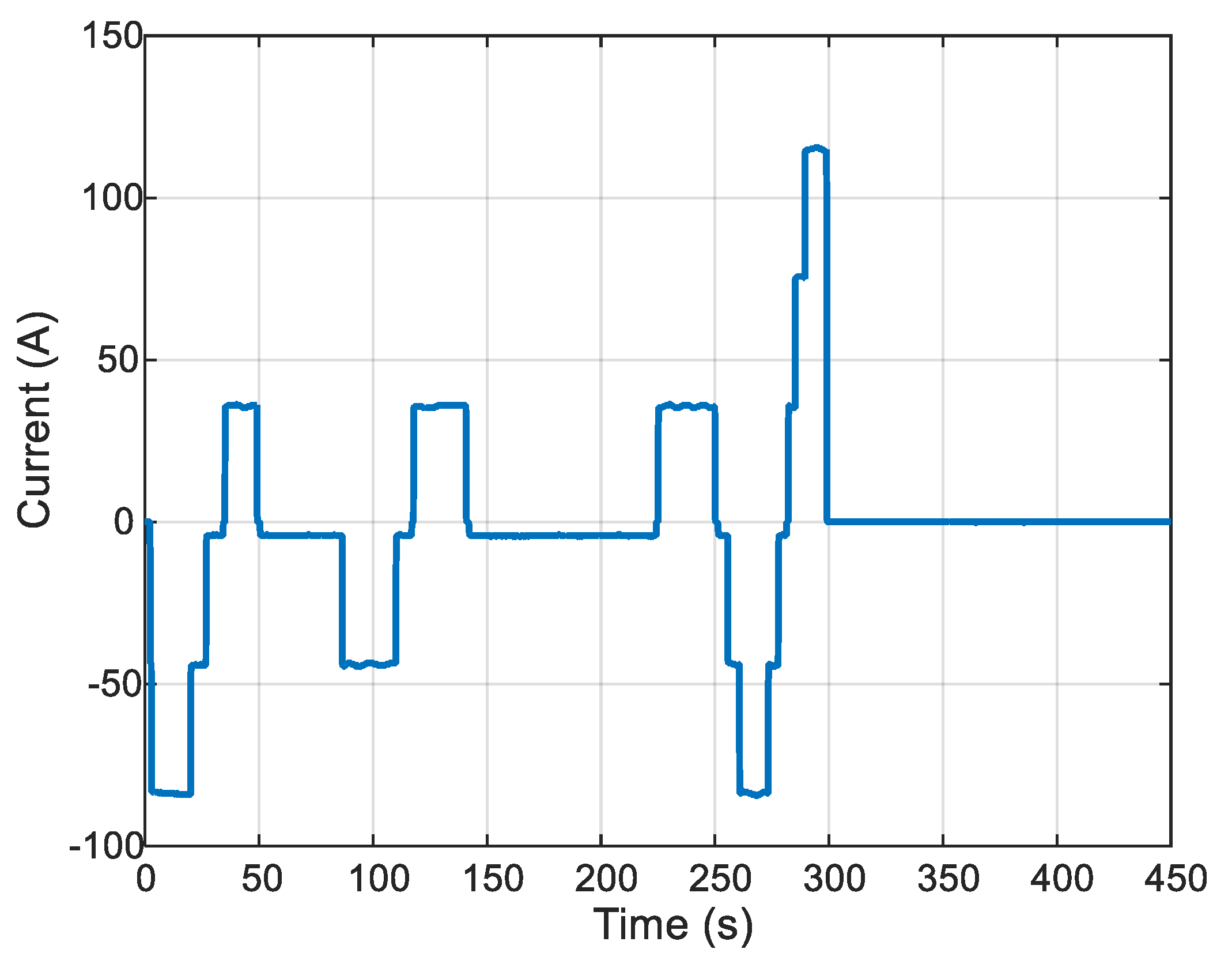
A system S_d models the diffusion of lithium in the spherical particle and links the current $I\left(t\right)$ to the concentration of lithium $C_s\left(t\right)$ at the surface of the spherical particle;

-

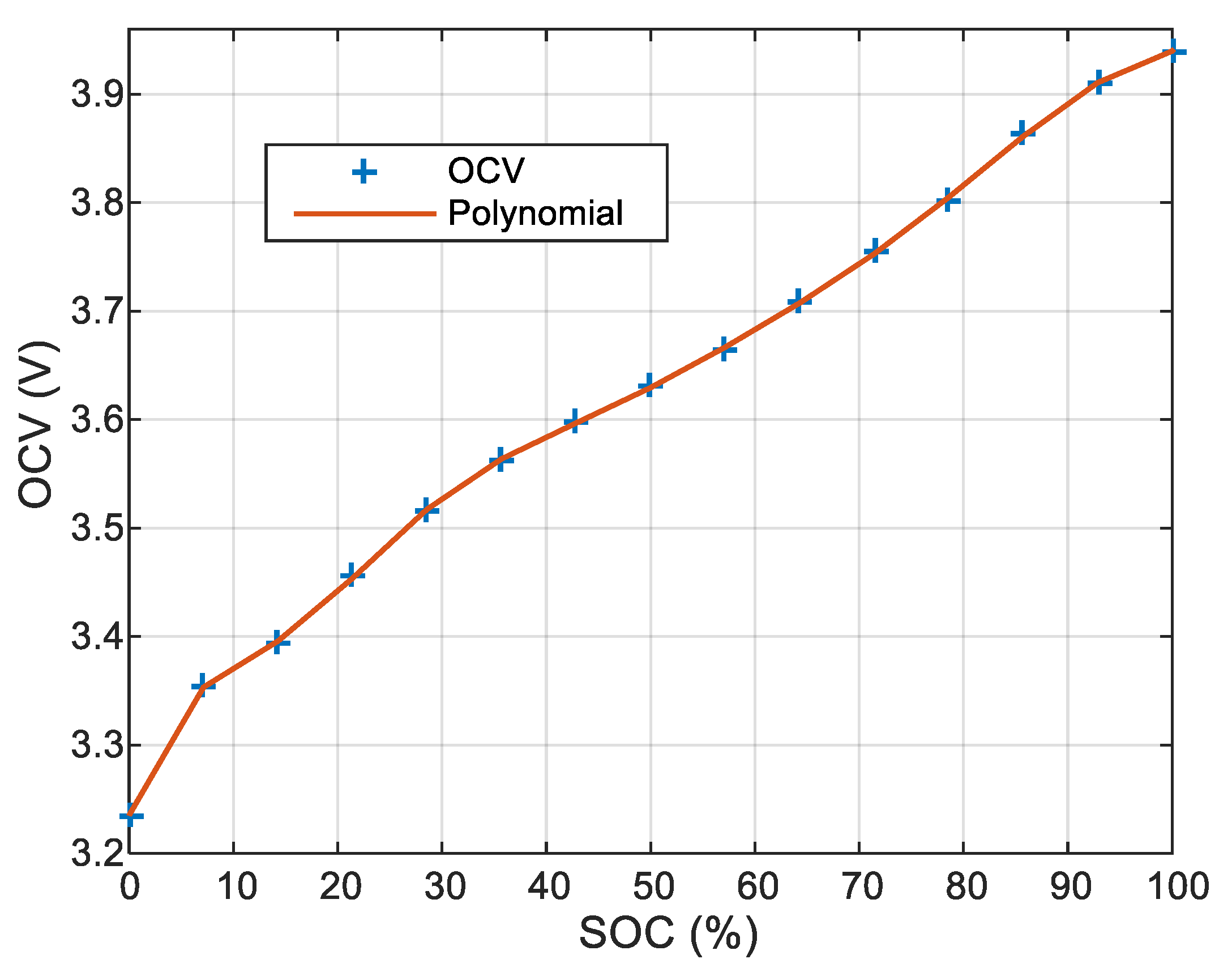
A nonlinear function $OCV\left(t\right)=f\left(C_S\left(t\right)\right)$ links the concentration of lithium at the surface of the spherical particle $C_S\left(t\right)$ to the open circuit voltage $OCV\left(t\right)$;

-

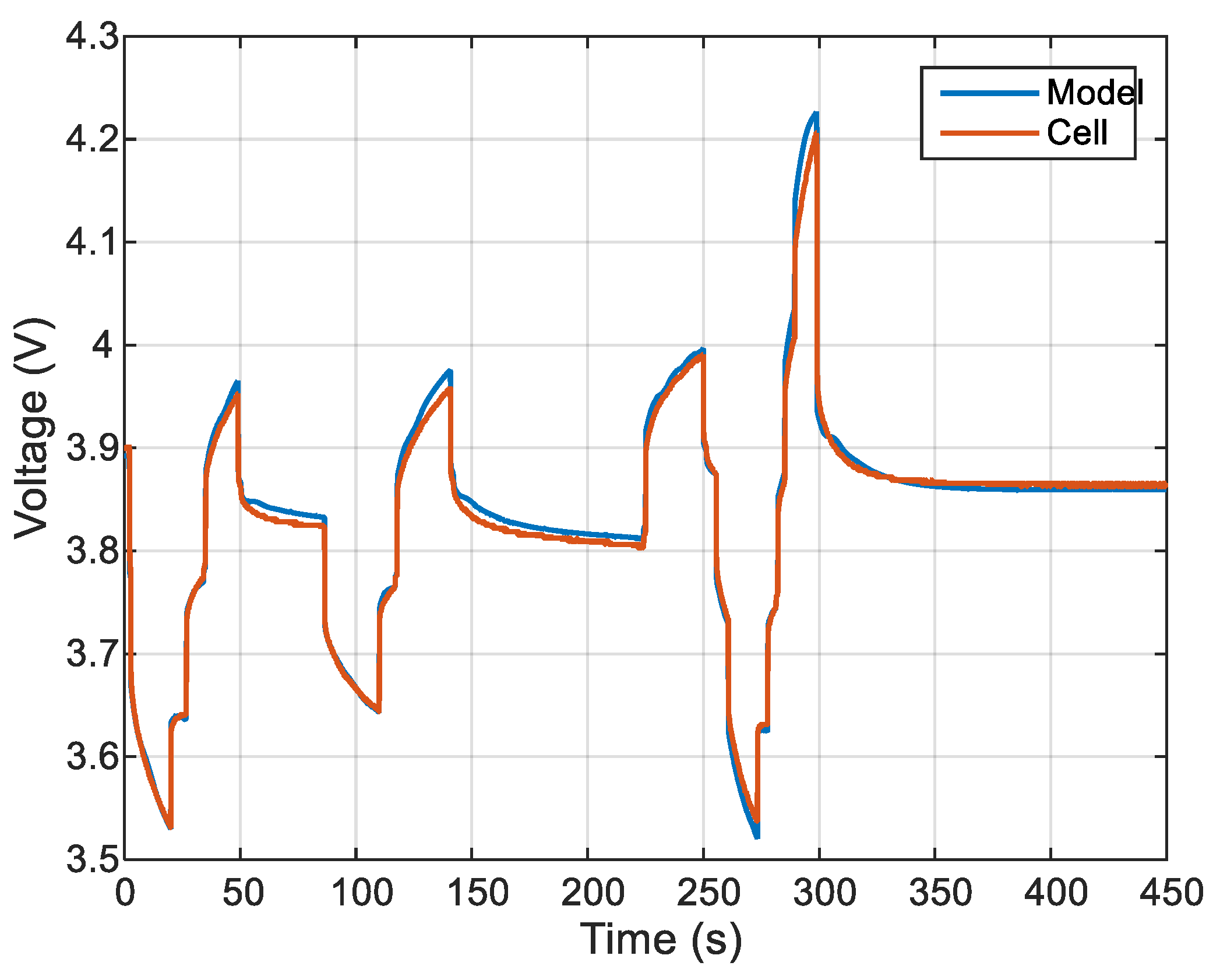
A resistor R is used to model the cell internal resistance and contact resistance.

The function $OCV\left(t\right)=f\left(C_s\right)$ can be obtained by measuring the cell voltage at rest for various cell states of charge (SOC). For the considered cell, this function is shown in Figure 8 and fitted by a degree 10 polynomial. The initial state of the battery is defined by $C_S\left(0\right)$ and the cell voltage is $U\left(t\right)$.

The diffusion part exhibits a power law behavior at high frequency and it is proposed here to model it using the following model:

$$\{\begin{array}{c}\frac{d}{dt}x\left(t\right)=A_1{{\displaystyle \int }}_0^{T_f}\eta \left(\tau \right)x\left(t-\tau \right)d\tau +BI\left(t\right)\\ U\left(t\right)=A_1{{\displaystyle \int }}_0^{\mathrm{t}}x\left(\tau \right)d\tau \end{array}$$

(22)

in which the kernel $\eta \left(\tau \right)$ is defined by Equation (16) with ${\omega }_l=10/T_f$ and ${\omega }_m$ chosen ten times greater than the sampling frequency of the current and voltage signals.

The current profile of Figure 9 is applied to the cell, and the parameters of Model (22) are tuned using a nonlinear optimization algorithm that aims to reduce the error between the measured voltage and the model output in Figure 7.

The parameter optimization process provides the following results for the Model:

$$A_1=989.6,B=45.92,T_f=1410\mathrm{s}$$

(23)

Figure 10 shows a comparison of the cell voltage and the voltage provided by the model. It reveals a good accuracy of the model and confirms the ability of this class of model to capture long memory power law type behaviors. The differences that appear are the result of the very high currents applied to the cell that exhibit some non-linear behaviors not taken into account by the model used.

5. What Does the Proposed Approach Solve?

The previous sections show that the class of distributed delay models considered (Equation (3)) is able to exhibit a power law behavior on a controlled frequency band. In comparison with the fractional Model (2), and in relation with the comments in the introduction section:

• In Equation (3), the variable $x\left(t\right)$ can be viewed as a real state and a physical meaning can be associated to it;
• There is no longer any ambiguity in the operator used for the definition of Equation (3) (in Equation (2), the Caputo, Riemann–Liouville, or other operators [12] can be chosen);
• The memory of Model (3) is of finite length;
• Initialization the Model (3) requires the knowledge of its state on a finite length and is well defined.

6. Conclusions

Dynamic systems that exhibit power law behaviors are currently modeled in the literature using fractional models. Several papers recently revealed various limitations of this class of model. In order to overcome these limitations, this paper is a first attempt to show that power law behaviors can also be captured by classes of models that were introduced into the literature some time ago, i.e., distributed delay models [26,27] (but also the Volterra equation of the second kind [28,29]). Two delay weight functions permitting the desired power law are proposed. First, a simple one, but with a singularity, and a second one without. For these two functions, conditions on the model coefficients are given for the definition of the frequency band on which the power law takes place. The class of model considered is used to capture the input-output behavior of a lithium-ion cell, a system that is known to exhibit a power law behavior.

The author intends now to study in greater detail the properties of this class of model in order to reach more complex behaviors. Particular attention will be paid to the meaning that can be given to the state in a modeling approach. Other classes of model will also be used.

References

1. Rodrigues, S.; Munichandraiah, N.; Shukla, A.K. A review of state-of-charge indication of batteries by means of a.c. impedance measurements. J. Power Sources 2000, 87, 12–20. [Google Scholar] [CrossRef]
2. Sabatier, J.; Aoun, M.; Oustaloup, A.; Gregoire, G.; Ragot, F.; Roy, P. Fractional system identification for lead acid battery state charge estimation. Signal Process. 2006, 86, 2645–2657. [Google Scholar] [CrossRef]
3. Cugnet, M.; Laruelle, S.; Grugeon, S.; Sahut, B.; Sabatier, J.; Tarascon, J.M.; Oustaloup, A. A mathematical model for the simulation of new and aged automotive lead-acid batteries. J. Electrochem. Soc. 2009, 156, A974–A985. [Google Scholar] [CrossRef]
4. Sabatier, J.; Merveillaut, M.; Francisco, J.M.; Guillemard, F.; Porcelatto, D. Lithium-ion batteries modeling involving fractional differentiation. J. Power Sources 2014, 262, 36–43. [Google Scholar] [CrossRef]
5. Battaglia, J.L.; Cois, O.; Puigsegur, L.; Oustaloup, A. Solving an inverse heat conduction problem using a noninteger identified model. Int. J. Heat Mass Transf. 2001, 44, 2671–2680. [Google Scholar] [CrossRef]
6. Malti, R.; Sabatier, J.; Akçay, H. Thermal modeling and identification of an aluminum rod using fractional calculus. IFAC Proc. 2009, 15, 958–963. [Google Scholar] [CrossRef] [Green Version]
7. Magin, R.L. Fractional Calculus in Bioengineering; Begell House Publishers Inc.: Danbury, CT, USA, 2006. [Google Scholar]
8. Mainardi, F. Fractional Calculus and Waves in Linear Viscoelasticity; Imperial College Press: London, UK, 2010. [Google Scholar]
9. Matignon, D.; d’Andrea-Novel, B.; Depalle, P.; Oustaloup, A. Viscothermal losses in wind instruments: A non-integer model. In Systems and Networks: Mathematical Theory and Applications; Akademie Verlag: Regensburg, Germany, 1994. [Google Scholar]
10. Enacheanu, O. Modélisation Fractale des Réseaux Électriques. Ph.D. Thesis, Université Joseph Fourier—Grenoble I, Grenoble, France, October 2008. Available online: http://www.theses.fr/2008GRE10159 (accessed on 20 November 2019).
11. Samko, S.G.; Kilbas, A.A.; Marichev, O.I. Fractional Integrals and Derivatives: Theory and Applications; Gordon and Breach Science Publishers: Philadelphia, PA, USA, 1993. [Google Scholar]
12. De Oliveira, E.C.; Tenreiro Machado, J.A. A Review of Definitions for Fractional Derivatives and Integral. Math. Probl. Eng. 2014, 2014, 6. [Google Scholar] [CrossRef] [Green Version]
13. Sabatier, J.; Merveillaut, M.; Malti, R.; Oustaloup, A. On a Representation of Fractional Order Systems: Interests for the Initial Condition Problem. In Proceedings of the 3rd IFAC Workshop on “Fractional Differentiation and its Applications” (FDA’08), Ankara, Turkey, 5–7 November 2008. [Google Scholar]
14. Sabatier, J.; Merveillaut, M.; Malti, R.; Oustaloup, A. How to Impose Physically Coherent Initial Conditions to a Fractional System? Commun. Nonlinear Sci. Numer. Simul. 2010, 15, 1318–1326. [Google Scholar] [CrossRef]
15. Ortigueira, M.D.; Coito, F.J. Initial conditions: What are we talking about? In Proceedings of the Third IFAC Workshop on Fractional Differentiation, Ankara, Turkey, 5–7 November 2008. [Google Scholar]
16. Sabatier, J.; Farges, C.; Trigeassou, J.C. Fractional systems state space description: Some wrong ideas and proposed solutions. J. Vib. Control 2014, 20, 1076–1084. [Google Scholar] [CrossRef]
17. Sabatier, J.; Farges, C. Comments on the description and initialization of fractional partial differential equations using Riemann-Liouville’s and Caputo’s definitions. J. Comput. Appl. Math. 2018, 339, 30–39. [Google Scholar] [CrossRef]
18. Sabatier, J.; Farges, C.; Merveillaut, M.; Feneteau, L. On observability and pseudo state estimation of fractional order systems. Eur. J. Control 2012, 3, 1–12. [Google Scholar] [CrossRef]
19. Atangana, A.; Baleanu, D. New fractional derivatives with nonlocal and non-singular kernel: Theory and application to heat transfer model. arXiv 2016, arXiv:1602.03408. [Google Scholar] [CrossRef] [Green Version]
20. Caputo, M.; Fabrizio, M. A New Definition of Fractional Derivative without Singular Kernel. Prog. Fract. Differ. Appl. 2015, 1, 73–85. [Google Scholar]
21. Dokumetzzidis, A.R. Magin, A commentary on fractionalization of multi-compartmental models. J. Pharm. Pharm. 2010, 37, 203–207. [Google Scholar]
22. Delfour, M.C.; Mitter, S.K. Controllability, observability and optimal feedback of affine hereditary systems. SIAM J. Control 1972, 10, 298–328. [Google Scholar]
23. Sabatier, J.; Rodriguez Cadavid, S.; Farges, C. Advantages of limited frequency band fractional integration operator in fractional models definition. In Proceedings of the Conference on Control, Decision and Information Technologies, CoDIT 2019, Paris, France, 23–26 April 2019. [Google Scholar]
24. Allagui, A.; Zhang, D.; Elwakil, A.S. Short-term memory in electric double-layer capacitors. Appl. Phys. Lett. 2018, 113, 253901. [Google Scholar] [CrossRef]
25. Sabatier, J.; Francisco, J.; Guillemard, F.; Lavigne, L.; Moze, M.; Merveillaut, M. Lithium-ion batteries modelling: A simple fractional differentiation based model and its associated parameters estimation method. Signal Process. 2015, 107, 290–301. [Google Scholar] [CrossRef]
26. Fridman, E. Introduction to Time-Delay Systems: Analysis and Control; Birkhauser Verlag: Basel, Switzerland, 2014. [Google Scholar]
27. Driver, R.D. Existence and stability of solutions of a delay-differential system. Arch. Ration. Mech. Anal. 1962, 10, 401–426. [Google Scholar] [CrossRef]
28. Grossman, S.I.; Miller, R.K. Perturbation theory for Volterra integrodifferential systems. J. Differ. Equ. 1970, 8, 457–474. [Google Scholar] [CrossRef] [Green Version]
29. Burton, T.A. Stability theory for Volterra equations. J. Differ. Equ. 1979, 32, 101–118. [Google Scholar] [CrossRef] [Green Version]
30. Abramowitz, M.; Stegun, I.A. Handbook of Mathematical Functions with Formulas, Graphs, and Mathematical Tables; Dover Publications Inc.: Mineola, NY, USA, 1965. [Google Scholar]
Figure 1. Gain (a) and phase (b) diagrams of integral I(s) for various values of ν and Tf = 10,000.
Fractalfract 04 00001 g001
Figure 2. Gain (a) and phase (b) diagrams of integral I(s) for various values of Tf and ν = 0.5.
Fractalfract 04 00001 g002
Figure 3. Impact of parameters ν, α0, and α1 on the gain of Model (14) denominator.
Fractalfract 04 00001 g003
Figure 4. Gain (a) and phase (b) diagrams of H(s)/s for various values of ν.
Fractalfract 04 00001 g004
Figure 5. Frequency response (gain on the (a), phase on the (b)) of I(s) with the non-singular kernel η(t) for ν varying from 0.1 to 0.9 and with ω l = 10 2 rd/s, ω m = 10 4 rd/s.
Fractalfract 04 00001 g005
Figure 6. Frequency response H(s) for various values of α 0 = 1 / ω 1 ν , with ν = 0.5: gain (a) and phase (b).
Fractalfract 04 00001 g006
Figure 7. Model of a lithium-ion cell proposed in [25].
Fractalfract 04 00001 g007
Figure 8. Considered cell open circuit voltage (OCV) fitted by a degree 10 polynomial.
Fractalfract 04 00001 g008
Figure 9. Current profile applied to the cell.
Fractalfract 04 00001 g009
Figure 10. Comparison of the cell voltage and the voltage provided by the model.
Fractalfract 04 00001 g010