Article

Fractal Image Interpolation: A Tutorial and New Result

Canaan Semiconductor Limited, Hong Kong, China
*
Author to whom correspondence should be addressed.
These authors contributed equally to this work.
Fractal Fract. 2019, 3(1), 7; https://doi.org/10.3390/fractalfract3010007
Submission received: 16 December 2018 / Revised: 13 February 2019 / Accepted: 20 February 2019 / Published: 23 February 2019

Abstract

:
This paper reviews the implementation of fractal based image interpolation, the associated visual artifacts of the interpolated images, and various techniques, including novel contributions, that alleviate these awkward visual artifacts to achieve visually pleasant interpolated image. The fractal interpolation methods considered in this paper are based on the plain Iterative Function System (IFS) in spatial domain without additional transformation, where we believe that the benefits of additional transformation can be added onto the presented study without complication. Simulation results are presented to demonstrate the discussed techniques, together with the pros and cons of each techniques. Finally, a novel spatial domain interleave layer has been proposed to add to the IFS image system for improving the performance of the system from image zooming to interpolation with the preservation of the pixel intensity from the original low resolution image.

1. Introduction

The Fractal Image Interpolation refers to image interpolation that makes use of the Partitioned Fractal Image (PFI) representation based on an Iterative Function System (IFS). When PFI representation is first introduced in the 1980s, there was a great deal of hope and excitement over the application of fractals to compress natural images, and fractals have spurred a considerable amount of research activities in that period of time. Although fractal image coding is no longer considered to be a competitive method to compress images because the compression ratio is not good enough, it is worth studying it as an alternate type of an image interpolation scheme because of the natural looking interpolation results. Within the IFS framework, images are modeled as deterministic fractal objects approximated by different parts of the same image, which is a direct result of the image being self-similar. The word “partition” comes in from the fact that the image is partitioned into blocks, and the search of self-similar fractal objects are performed over all the partitioned blocks that covers the whole image. As a consequence of the self-similarity, the fractal objects are scale independent. In the IFS framework, the fractal objects are described with a simple recursion, such that images with different sizes (scales) can be generated from the associated fractal codes using the same recursion. This property makes changing image resolutions in PFI very easy [1].
Despite the mathematical simplicity in scaling images in PFI, the PFI is a block based image processing algorithm, therefore, just like other block based image interpolation algorithms presented in literature, PFI based image interpolation suffers from a blocking artifact. All methods that deal with the blocking artifact in other block based image interpolations are applicable in PFI based image interpolation. Despite the very complex theoretical background of the PFI based image interpolation method, the objective performance of the interpolated images may not be as good as those images interpolated by other methods presented in literature. However, the PFI based image interpolation usually achieves good subjective performance, which is one of the reasons why fractal image interpolation algorithms have been adopted into many commercial image enlargement software, and is still actively investigated in literature [2,3,4,5,6]. It has been reported in [7,8] that, for some image interpolation applications, such as medical image interpolation, the preservation of image shape (structure) is far more important than the objective quality of the interpolated image. As a result, Ref. [7] has proposed the application of IFS based image interpolation for medial image interpolation. Recently, fractal image interpolation has also found applications in other fields, such as image encryption [9] and depth map interpolation in 3D computer graphic [10], etc. Disregarding their very different applications, the core of these algorithms are the basic PFI, which will be discussed in later sections in this paper.
It is the purpose of this paper to review fractal image interpolation from the basics of IFS and to present the mathematical analysis on various techniques that have been presented in literature to alleviate various shortcomings of the fractal image interpolation. Furthermore, novel techniques will be presented to show how to make use of fractal based interpolation to achieve natural looking interpolated images of high visual quality. Finally, we shall propose the insertion of a spatial interleave layer into the IFS decoder to enable the preservation of original low resolution image pixel intensity in the interpolated image for both better objective and subjective interpolated image qualities.
The rest of this paper is arranged to present the basic theory of the IFS in Section 2, which will also demonstrate the zoom-in property of the IFS. Section 2 will present the partitioned IFS (PIFS) and show how to make it represent natural images. A particular implementation of the fractal image encoder and decoder will be presented in Section 3 and Section 4, respectively. A demonstration on how to make use of the decoder function to zoom-in an image will be presented in Section 5. The technique that helps to modify the PIFS zooming to PIFS interpolation will be presented in the same section. The block overlap based image interpolation method will be presented in Section 6, which helps to alleviate the blocking artifacts observed in the PIFS interpolated images. This paper concludes in Section 7.

2. Iterated Function System

The fractal can be defined in a number of ways depending on the applications. When applied in image interpolation, we are interested in fractals defined by the IFS. We shall not go through the complex mathematical derivation, and shall take it for granted that the contraction affine transformation can generate fractals, and hence forms an IFS. By repeating the contraction affine transformation an infinite number of times, any starting patterns will be transformed into the same structure at any level of details. In other words, the IFS allows us to zoom (interpolate) into the details of the structure. Having said that we shall skip the complex mathematics, the basic mathematical tools and theorems about fractals defined by the IFS are revisited to make this review complete.

2.1. Fixed Point Theorem

The convergence of the IFS defined by a contraction transformation is the result of the “Fixed Point Theorem”. In here, we shall discuss the most basic Fixed Point Theorem in analysis, which is due to Banach and appeared in his Ph.D. thesis (1920, published in 1922) [11].
Theorem 1. Fixed Point Theorem:
Given a complete metric space ( X , d ) and a transformation T : X X that satisfies
d ( T ( x ) , T ( y ) ) c · d ( x , y ) ,
for some 0 c < 1 and all x , y X . The transformation T has a unique fixed point x f in X, where given any x 0 X , the sequence that iterates on x 0 , T ( x 0 ) , T ( T ( x 0 ) ) , converges to the fixed point x f of T.
The Fixed Point Theorem is also known as the Banach Fixed Point Theorem, and Contraction Transform Theorem. The transformation T that satisfies the Fixed Point Theorem is known as contraction mapping. A contraction shrinks the distance by a uniform factor c of less than 1 for all pairs of points. To get a grasp on the application of the Fixed Point Theorem, we shall review a high school problem of finding a high accuracy approximation to the irrational number 5 by Newton’s method. Newton’s method provides a scheme to construct the contraction transform where the associated fixed point is the solution of a system of equations.
Example 1.
The solution of the equation f ( x ) = 0 , with f being differentiable can be approximated by Newton’s method, finds an approximate solution x 0 and then computes the following recursive sequence
x n = x n 1 f ( x n 1 ) f ( x n 1 ) .
The contraction transform is given by
T ( x ) = x f ( x ) f ( x ) .
Starting from some initial point x 0 , the recursion will converge to T ( x f ) = x f , a fixed point of T ( x ) . When that happens, we shall have T ( x f ) = x f = x f f ( x f ) f ( x f ) , which implies f ( x f ) = 0 . In other words, the fixed point x f is a solution of f ( x ) = 0 .
To use Newton’s method to estimate 5 , we shall set f ( x ) = x 2 5 and seek a (positive) root of f ( x ) . The Newton recursion is thus given by
x n = x n 1 x n 1 2 5 2 x n 1 = 1 2 x n 1 + 5 x n 1 .
Hence, the contraction transform is given as
T ( x ) = 1 2 x + 5 x .
The fixed point of T is 5 . Table 1 listed x n obtained in each iteration of Equation (4) with different initial value x 0 . All of the sequences with different x 0 are observed to converge to 2.236068 5 . On the other hand, the number of iterations required for each sequence to converge are observed to be different. In fact, the number of iterations required for the sequence to convergence depends on the distance between x 0 and 5 .
Example 1 not only forms an IFS that converges to 5 . A closer examination will reveal the fact that the number 5 is now represented by the contraction transform in Equation (5). In fact, any number a can be approximated with an IFS defined by Equation (5) with a simple change of variable. If we use a polynomial representation system to describe the corresponding IFS, Equation (5) can be rewritten as ( 0.5 , ( 1 , a ) , ( 1 , 1 ) ) , where the first coefficient 0.5 is the scaling, or magnitude transformation. The following two-tuple list the order of x and the corresponding coefficients. As an example, the tuple ( 1 , a ) represent the term a x . This polynomial representation provided us an alternative way to describe the number a , and is a more efficient (compact) way to store the number a , which by definition would require an infinite space to store all the decimal places. Such representation also provides us a way to zoom into a . The accuracy of approximation to a depends on the number of iterations applied to compute Equation (5). More details of a can be revealed if we allow Equation (5) to iterate a few more times. This detail “zoom-in” property is what makes IFS an interesting image interpolation method. The image interpolation problem can be casted as the problem of finding the contraction transform that forms an IFS with the associated fixed point approximating a given image. After that, we can make use of the contraction transform and the associated IFS to zoom into the details of the fixed point, which will provide us with an interpolated image.

2.2. Partitioned Iterative Function System
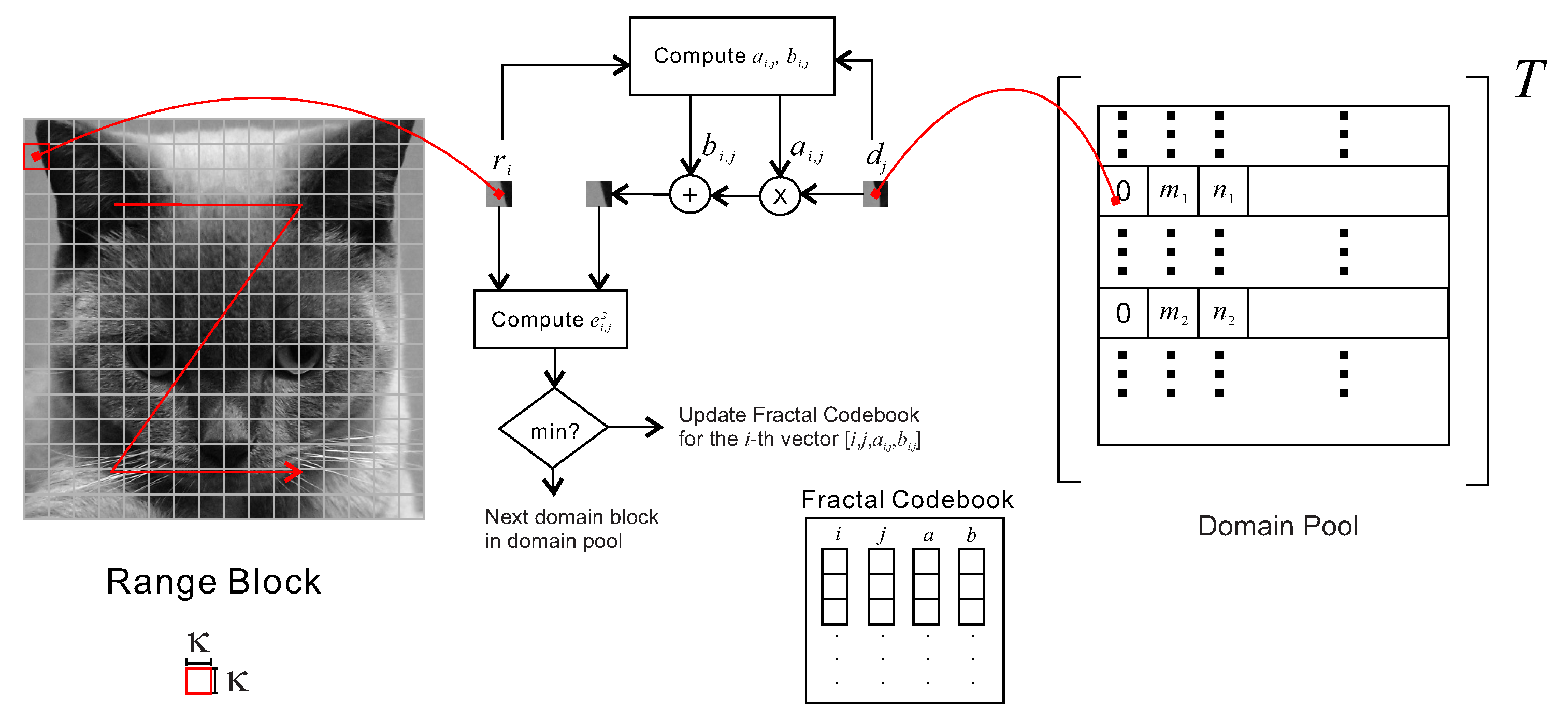
The direct application of the IFS would suggest the representation of any given image as a contraction transformation of itself. Among various methods that extend the Fixed Point Theorem to handle digital images, the conventional PIFS consider linearizing the partitioned image block to a vector of size N in R N , such that the contraction transform is a mapping from R N R N . Among various methods to construct the contraction transform, we are particularly interested in the Affine Transform defined as
Definition 1. Affine Transform:
The affine transform in R N R N defined as T ( x ) = A x + b with x , b R N and A R N × N .
The contractivity of the Affine Transform is given by Theorem 2.
Theorem 2.
The affine transform in T ( x ) : R N R N is a contraction transform, with respect to the norm R N that induces the matrix norm when
| T | < 1 ,
with a given matrix norm.
Theorem 2 can be easily proved by considering x , y R N ; then, | T ( x ) T ( y ) | = | A ( x y ) | | A | · | x y | = | A | · d ( x , y ) , which implies T is contractive by Theorem 1. According to Hutchinson [12], given a collection Ω of affine and contraction transforms T i , with i = 1 , 2 , , in a complete metric space ( R N , d ) , the following union of contraction transforms
T = i = 1 T i , T i Ω
is also a contraction transform. The IFS fractal image representation makes use of the super-position of all small fixed point of each contraction transform T i to approximate a given image. Such system represented by Ω is known as a Partitioned Iterated Function System (PIFS) because the image is being partitioned into blocks and each partitioned blocks are being represented by a contraction transform T i . Such an image representation is shown to be more efficient. This is because natural images do not satisfy self-similarity in a strict sense, many images (particularly photographs), such as the Cat image as shown in Figure 1a which has some areas that are almost self-similar but also has some distinct areas. The similarity of parts of an image provides the inspiration for the concept of a PIFS, which is a block based fractal image representation scheme that exploits local self-similarities within the image [13]. The PIFS is similar to an IFS, except that the contraction transforms have restricted domains that exploit the inherent local self-similarities of the image. The flexibility of PIFS permits the construction of a more general measures such that the image to be transformed does not have to be strictly self-similar [14]. In practice, this means that an image f can be represented by PIFS with N r partitioned small regions, or also known as range blocks, r i , that spans the image f,
f = i = 1 N r r i .
Each of the r i is matched as closely as possible to the affine transform of one of several larger regions, known as domain blocks, d j : j = 1 , , N d of the image. It should be noted that each range block can be considered as sub-images, in which the indices i and j refer to the order of the range blocks and domain blocks in their corresponding collections, respectively. It is assumed that the blocks are ordered according to their appearance in the original image following by row and then column. Each range block will be matched against all the domain blocks in the original image. The best match result yields the contraction transformation, T i , that maps part of the original image onto that range block r i . A PIFS encodes N r sub-images r i , where the fixed point associated contraction transform T i for each r i will then be super-imposed to produce a single image. As a result, the union of the contraction transforms is sufficed to represent the fixed point image, which in turn is an approximation of the original image.
f f f = i = 1 N r T i ( d α ( i ) ) ,
where α ( i ) is the mapping that gives the best domain block index for the i-th range block. With reference to the contractive mapping fixed point theorem, the union of contractive mappings in Equation (9) has a unique fixed point, f f , called the attractor of the PIFS. Therefore, if we can find a PIFS such that its attractor is as close to the image f as possible, we can obtain a good approximation of the image f and represent it with a union of affine transforms. Furthermore, the Fixed Point Theorem tells us that the iterations of finding f k + 1 = i = 1 N r T i ( d k , α ( i ) ) is a convergent series, where d k , j is the j-th domain block extracted from the image f k obtained at the k-th iteration. Starting with any arbitrary initial f 0 , the series will converge to the unique fixed point f f . A natural solution to find T i and α ( i ) for the PIFS representation of f with the contraction transform constrained to be affine transform defined in Theorem 2 can be obtained by rewriting Equation (9) as
f f = i = 1 N r ( A i d α ( i ) + b i ) = i = 1 N r P i ( A i d α ( i ) + b i ) = i = 1 N r P i j = 1 N d ( A i S i , j ) f f + b i = A f f + b ( A I ) f f = b f f = ( A I ) 1 b ,
where P i ( · ) is the translation operator that putting the affine transformed domain block to the i-th range block position, and S i , j is the domain block extraction operator that extracts the α ( i ) -th domain block with S i , j = 1 when j = α ( i ) , otherwise, S i , j = 0 when j α ( i ) . The matrix A gathered all the matrix products of P i ( A i S i , j ) together, and b is a matrix that lumped all the translated scalar P i ( b i ) together to form a matrix in the size same as that of the image matrix f. If the fixed point f f converges to the original image f exactly, Equation (10) can be rewritten as f = ( A I ) 1 b . In other words, the PIFS is now posed as an inverse problem for finding A and b as shown in Equation (10), where ( A , b ) serves as the fractal representation for f. However, solving this inverse problem is difficult. In particular, most real-world objects are rarely entirely self-similar. As a result, f f f , and hence the inverse problem in Equation (10) is ill-posed. Fortunately, Barnslay shows that we don’t have to solve the inverse problem. A good PIFS representation with f f that approximates f can be found by the application of Collage Theorem [14].
Theorem 3. Collage Theorem:
Given an IFS with contraction transform T in the complete metric space ( X , d ) , contraction factor c ( 0 , 1 ) , and fixed point X f . Let X and ϵ > 0 be chosen such that
d ( X , T ( X ) ) ϵ ,
then
d ( X , X f ) ϵ 1 c .
According to the Collage Theorem, the closer is the collage T ( f ) (first-order approximation of the fixed point) to the original image f, the better is the constructed PIFS, and hence the attractor f f is closer to the original image f. In other words, when constructing the PIFS (the fractal encoding process), one can focus on minimizing the d ( f , T ( f ) ) , and this will result in minimizing the d ( f , f f ) , which is the goal of fractal representation of the original image f. The quantitative distance measure metric d ( f , T ( f ) ) is called the collage error. The computational complexity of fractal representation is significantly reduced by the minimization of the collage error instead of the distance between the original image and the attractor (the fixed point f f ), i.e., d ( f , f f ) . With respect to each range block r i f , the PIFS is constructed by finding the domain block d j and the corresponding affine transform matrix A i and b i that satisfies
d ( r i , T ( d j ) ) = min j , A i , b i d ( r i , A i d j + b i ) .
The above is a direct application of the Collage Theorem, a simple consequence of the Fixed Point Theorem, which ensures the fixed point f f is close to f if the distortion i = 1 N r d ( r i , T ( d j ) ) between the original image and its collage T ( d j ) is small. A union of these contraction transforms for all the partitioned blocks will form the PIFS. In other words, the PIFS is formed by the set of surjective functions that maps the j-th domain block to the i-th range block. The procedure that achieves the best match is known as the fractal encoding.
The mapping between i and j, the affine transform A i and the shift b i are sufficient to define the IFS. The collection of the i , j , A i , b i froms the fractal codes of the PIFS. However, this solution does not give the optimal results. It is vivid that the larger the block size of r i , the fewer the number of bits are required to store the fractal code and hence provides higher coding gain. On the other hand, the larger the block size, the poorer the fractal approximation (the fixed point) of the original image, and, hence, the lower the quality of the fractal encoded image. For the purpose of image interpolation, the fractal code is used to zoom into the image, where better fractal approximation is desired. Therefore, a small block size is preferred. However, the structural property advantages of fractal image representation can only be observed with large block size. This creates a design dilemma in choosing the right block size for better original image resemblance or better structural quality of the zoomed image. The subsequent section will show you that a block size of 4 × 4 and 8 × 8 will be sufficient depending on the interpolation ratio r.
The fractal image encoding method in Equation (13) is a simplified implementation of the first fully automatic method for fractal encoding presented by Jacquin [13], which forms the basis for many fractal encoding methods. All other methods can be treated as improvements to the Jacquin’s method. However, there are still a few practical issues left unaddressed before we can successfully implement a Jacquin fractal encoding method. The problems to be addressed include what kind of partitioning for the image should be used, and how does one find the best matching block pairs from the partitioned blocks and the associated grayscale transform that will optimally transform these best matching blocks for each range block. The above problems will be addressed in the following sections.

3. Encoding

In the ideal case, the partition of the image should be performed according to the image structure to optimize encoding. However, such an intelligent approach would need a human to drive it. A fully automatic approach is only possible if a fixed partition of the image is applied. In a simple PIFS image encoder, the image is partitioned in two ways to generate the range blocks r i , often with uniform size and non-overlapping; and the domain blocks d i , with a larger size than that of the range blocks, and usually overlapping.

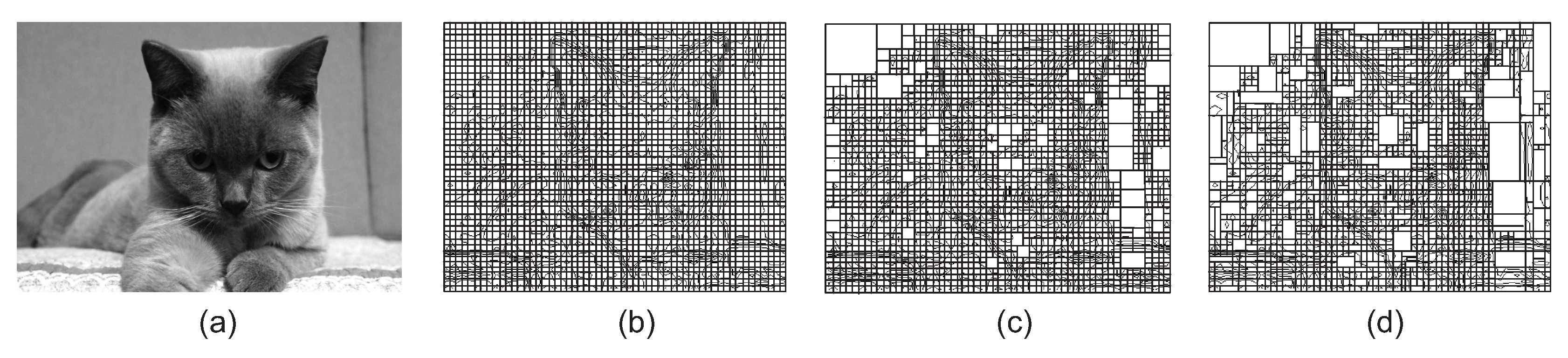
3.1. Range Block Partition

The image can be partitioned by different ways to obtain the range blocks, and they can be summarized into three major categories with the partitions shown in Figure 1 for the Cat image. Showing in Figure 1b is uniform partition, where all the blocks have the same size. An example to obtain the range block by uniformly partitioning the image array into distinct κ × κ block, and rearrange them as a column vector for storage. The total number of distinct blocks being partitioned from a M × N image array is given by M / κ × N / κ , and hence the total memory size required to store all range blocks is given by
( κ × κ ) · ( M / κ × N / κ ) .
Uniform partition is computationally efficient, but inefficient in terms of coding performance. Figure 1c is the quadtree partition, where the partitioned blocks are squares with adaptive sizes based on the information content of the localized image region. However, the gain provided by the quadtree partition in natural images is not compatible with the induced computational complexity, and is therefore not commonly found in commercial implementation. Figure 1d is the HV partition [15]. This is an advanced and efficient partition method that partitions the image into quadrangle blocks with adaptive sizes based on the information content of the localized image region. The HV partition should be the most efficient way to generate the range blocks. However, the HV partition has the deficiency of the possibility of leave out regions, such that a highly sophisticated algorithm is required to ensure the non-overlap partitioned blocks will fully cover the image. Therefore, HV partition is seldom used in practice. Other types of freely-shaped partitions [16] have also been applied to extract range blocks to form PIFS. Among them, the non-regularly shaped partition methods do have the same drawback as that of HV partition. The non-symmetrical (on either or both horizontal and vertical axes) partition will require the contraction transform to include necessary horizontal, vertical and/or diagonal flippings to order to create a codebook that can be shared by all the range blocks. One such kind of partition is the triangular partition [17]. However, as pointed out in [18], the increase in computational complexity and storage to extract the range without using uniform partition is simply too high, which prohibited their deployment in real world applications. The following discussion will concentrate on uniform partition, which provides sufficient information for us to investigate the problems of the fractal image interpolation and various techniques to alleviate the fractal image interpolation artifacts.

3.2. Domain Block Partition

While the range block is obtained by uniform partition, the most frequently used domain block partition strategy is uniform partition with overlap, which provides optimal partition result, but is also extremely computational expensive. The domain blocks are usually assumed to be twice the length and width (hence four times the size) of those of the range blocks, where the the size of each domain block is ( 2 × κ ) · ( 2 × κ ) . Since a domain block overlaps with its neighboring domain block with the difference of one pixel only, therefore, the total number of domain blocks of a M × N image is given by N d = ( M 2 × κ + 1 ) · ( N 2 × κ + 1 ) ) , and they are all stored column-by-column. In other words, the total number of columns is ( M 2 × κ + 1 ) · ( N 2 × κ + 1 ) . Therefore, the total memory size required to store all domain blocks is given by
( 2 × κ · 2 × κ ) · ( ( M 2 × κ + 1 ) × ( N 2 × κ + 1 ) ) .
To simplify the encoding process, the affine transform will be performed on all the domain blocks, and the transformed blocks will be stored in a domain pool ( P ). In this case, the PIFS image encoding process will become the process of finding a surjective function d j r i from a particular block d j in the domain pool P to the range block r i under consideration. This surjective function will find the best matching block from the domain pool P for each range block with respect to a given matching criteria. Various matching criteria can be applied which essentially affects the complexity and the quality of the fractal image representation. In the rest of the paper, the matching criteria applied to illustrate the theory and implementation of PIFS encoding is the L 2 distance between c i and r i . The mapping that provides the least squares distance will be the best matching pair. Naturally, the larger the domain pool, the better the matching between the domain blocks and the range blocks can be obtained. However, a large domain pool will require more memory to store the indices that specifying the locations of the best matched block in the domain pool. A similar observation is also reported in [6]. From a computation efficiency viewpoint, compromises between the domain pool size, domain block size, range block size, and the fidelity must be established.

3.3. Domain Pool Generation

The domain pool P is a collection of domain blocks. Since all the blocks in the domain pool will be compared with the range blocks, they should be size compatible. In other words, we have to either interpolate the range block to make it as big as that of the domain blocks, or down-sample the domain blocks to make it as small as that of the range blocks. It will be difficult if not impossible to prove either method to be theoretically optimal. As a result, the one that has the lower computational complexity will usually be adopted. The smaller the block size, the lower the computational complexity. Therefore, we shall adopt the approach of down-sampling the domain blocks to generate the domain pool. There exist a large number of image block down-sampling algorithms. To ease our discussions, we shall adopt the bilinear down-sampling method. Besides the down-sampled domain blocks, the domain pool can be enriched by incorporating various affine transformed down-sampled domain blocks as the domain pool vectors. While there are infinitely many different types of affine transformations that can be applied to enrich the content of the domain pool, the most frequently applied affine transformations for domain pool generation are the isometric affine transformations, which include four rotations, a horizontal flipping, a vertical flipping and two diagonal flippings, where all these transformations are isometries of the original decimated domain blocks [19]. To simplify the discussion, the implementation example to be presented will only concentrate on the domain pool generated with domain blocks directly extracted from the given image without performing any isometric affine transformation. In summary, the domain pool generation process begins with the partition of the original image into a serial of domain blocks. All the domain blocks in the image have the same block size.
The domain blocks are taken sequentially from the top-left corner of the image and slide through the image in a row-then-by-column manner, until the last domain block with the top-left corner pixel located at [ ( M 2 × κ + 1 ) , ( N 2 × κ + 1 ) ] is taken, such that all the pixels in the original image are covered. The top-left corner coordinate of the block extracted from the original image that forms the domain block, together with the affine transformed contents (in our case, the down-sampled domain blocks) will be stored in the domain pool P . As a result, a simple domain pool P that does not contain any isometric affine transform blocks will have ( M 2 × κ + 1 ) × ( N 2 × κ + 1 ) entries, where the total domain pool size is given by ( κ × κ ) · ( M 2 × κ + 1 ) · ( N 2 × κ + 1 ) . It should be noted that, when other isometric affine transformed blocks are also included in the domain pool, the number of entries of the simple domain pool will be concatenated with the affine transformed vectors.
It is believed that a large domain pool will result in very good PIFS image representation quality. However, a large domain pool will cost high computational complexity to find the best match block within the domain pool for a given range block. It has been shown in [6,20] that allowing more rotations and shrinking factors or more domain blocks will not improve the performance of the fractal image representation significantly.

3.4. Grayscale Scaling
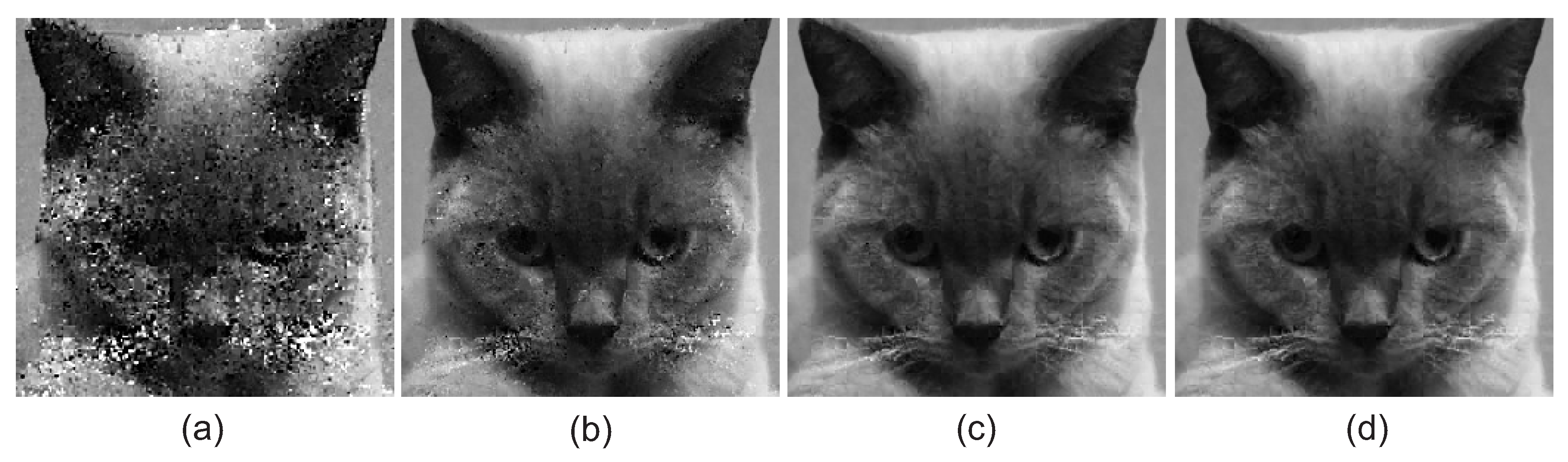
To complete the encoding of the image, the range block r i is matched with the domain block in P . To find the best match domain block d j for a given domain block, we have to scale and offset the domain block, where the optimal scaling and graylevel offset can be obtained with direct application of the Collage Theorem in Equation (11). The Collage error e i , j of the domain block d j in the P for the range block r i given by
e i , j 2 = min a i , j , b i , j r i ( a i , j · d j + b i , j ) 2 .
The parameter pair ( a i , j , b i , j ) performs graylevel scaling and offset on the domain block d j to minimize the squares distance with the given range block r i . It should be noted that the a i , j and b i , j are both scalar and they are degenerated from A and b , respectively. These parameters can be easily found by solving the least squares problem with the optimal grayscale transform pair given by the solution of the linear equations (assuming a unique solution exists)
a i , j = ( κ × κ ) m , n ( r i [ m , n ] d j [ m , n ] ) ( m , n r i [ m , n ] ) ( m , n d j [ m , n ] ) ( κ × κ ) m , n d j 2 [ m , n ] ( m , n d j [ m , n ] ) 2 ,
b i , j = m , n r i [ m , n ] a i , j m , n d j [ m , n ] κ × κ .
There is one complication, however, about the contractivity of the fractal transform operator T is dependent on the scaling coefficient a i , j . There is no simple relationship between the L 2 contractivity factor, a i , j , and b i , j because of the local nature of the surjective mapping. However, in the L norm, contractivity is guaranteed if all the grayscale scaling factors a i , j associated with all range blocks satisfy the condition | a i , j | < 1 . For this reason, most fractal coding algorithms “clamp” the coefficients a i , j to be a = s i g n ( a i , j ) · min ( | a i , j | , 1 ) . As a result, the associated fractal transform is contractive in L , hence almost always contractive in L 2 , due to the equivalence of the norms in finite pixel space.
The optimal grayscale transform of each range block is computed for each domain block inside the simple domain pool P in order to find the closest domain block to each range block. This optimality search is performed by storing all Collage errors e i , j for all d j in the P with a given range block r i . These stored Collage errors will be compared and the minimum is chosen where the associated surjective mapping i j forms the contraction transform. These surjective mapping pair ( i , j ) for all i that cover the image, together with the grayscale scaling parameter pair ( a i , j , b i , j ) , will form the complete PIFS to describe the input image. The 4-tuple ( i , j , a i , j , b i , j ) is also known as the fractal code. With the 4-tuples are stored in predetermined orders associated with i, it is possible to simplify the 4-tuples to a 3-tuples ( j , a , b ) . In particular, the 3-tuples are what we needed to construct the PIFS representation for the given image.
Figure 2 is the summary of the fractal encoding process. The original image is partitioned into a serial of range blocks. For simplicity, the ordering of the range blocks are made exactly the same as that of the domain blocks, but the block size of the range block is smaller than that of the domain blocks. All entries in the simple domain pool P will be considered in the encoding for each of the range block r i . However, in the example, the size of the row and column dimensions of the domain block are both twice those of the range block, the block content of the domain block is down-sampled to form d j , which has the same block size as that of the range block r i . Both r i and d j are applied in the generation of the graylevel scaling a i , j and offset b i , j parameters. The adjusted c j will be compared with r j for the Collage error e i , j 2 . The encoding of that particular r i will be accomplished when the minimum e i , j 2 is achieved. The row coordinate and column coordinate of d j gives minimum e i , j 2 for r i will be stored in the i-th element in the column vectors i and j, respectively. The corresponding a i , j and b i , j will be stored in the i-th element in the column vectors a and b, respectively. The four column vectors that contain i, j, a and b are the fractal codebook. It should be noted that the i-th elements in the fractal codebook will be updated when a smaller e i , j 2 comes in. The encoding process for range block r i will be done when all entries in the simple domain pool P are considered and the encoding will proceed to the next range block. The result of the fractal encoding process is presented in the form of the fractal code ( i , j , a i , j , b i , j ) for all range blocks. The collection of all the fractal codes is known as Fractal codebook. There are a lot of things that can be done with this fractal codebook. In the following sections, we shall first discuss how to reconstruct an approximated image f from the fixed point described by the fractal code ( i , j , a i , j , b i , j ) . We shall then extend the reconstruction result to create an interpolated image with interpolation ratio of 2.

4. Decoding

The fractal code generated by the PIFS encoding process described the relations between different parts of the image, which is independent from the size and resolution of the image. With a given fractal code that defines the collection of contraction transforms T (the affine transform described by the j-th domain block ( d j ) and the associated grayscale scaling and offset by ( a i , j , b i , j ) for the i-th range block), the fixed point f f can be obtained by simple iteration of the union of the contraction transforms. Starting with an arbitrary image f 0 , one forms the iteration sequence f k + 1 = T ( f k ) . With the contraction transform constrained to be simple affine transform as considered in previous section, the decoding procedure can be constructed by recovering the range blocks of the ( k + 1 ) -th decoded image f k + 1 from the simple domain pool P of the decoded image f k . A decoding loop of the above procedure will be performed until a specified quality parameter is fulfilled, and is detailed in the following steps.
  • Constructs the simple domain pool P using the down-sampled domain blocks from the previously decoded image. The domain pool generation routine should be the same as that used in the PIFS encoder. Furthermore, if there is no previously decoded image, the “previously decoded image” can be initialized by any image, including the dark image (i.e., all pixels have intensity equal zero). For image interpolation, the initial image can be the original image f, such as to reduce the decoding time (i.e., f 0 = f ).
  • Form the i-th range block from the j-th domain block extracted from the initial image with graylevel scaling by a and addition of brightness shift b on each pixel, where the parameters j, a and b are retrieved from the fractal code one-by-one from the codebook and generate the attractor image f, where each range blocks in f 1 are generated by applying grayscale scaling a and shifting b to the j-th domain block.
  • Glue all the range blocks together to form the fractal decoded image at the k-th iteration.
  • If the number of iteration is smaller than a predefined number, and, if the differences between the images in consecutive loops is larger than a specified tolerance, then go back to step 1 for the ( k + 1 )-th fractal decoding iteration using the k-th fractal decoded image as the start image.
This iterative decoding procedure does not require exhaustive search, nor matrix inverse computation, therefore, it is vivid that the decoding procedure requires a fraction of the computational complexity when compared to the fractal encoding procedure. Most of the computation time will be used to construct the simple domain pool P from the decoded image in each loop.
Figure 3 shows the decoded images with fractal encoding using a domain pool with block size of κ = 8 without isometric transform of a 256 × 256 8-bit grayscale Cat image. The fractal nature of the decoded image is vivid from Figure 3a, which is the decoded image obtained from the 3rd iteration. Blocks with similar features as that of the original image are being put together, and it is possible to identify the Cat image from Figure 3a. The image in Figure 3b is obtained with two more iterations. The Cat image is almost completely reconstructed from the PIFS decoding iterations. The decoded image obtained from the 7th iteration as shown in Figure 3c has already faithfully reconstructed the Cat image, and only a minimal difference can be found between the 7th iteration PIFS decoded image and that obtained from the 20th iteration PIFS decoded image as shown in Figure 3d.
Compared with the classical DCT based coder, the image Figure 4a obtained from fractal decoding with the Cat image encoded with κ = 8 , at the 20th iteration has a compression ratio compatible to that of the DCT image coding with 8 × 8 DCT block size and retaining only the 4 × 4 low frequency sub-block as shown in Figure 4b. Observed from Figure 4a, the fractal PIFS is superior in encoding edges as well as low frequency image content but lack perceivable texture. Due to the exploitation of scaling invariance (the domain blocks are scaled down by a factor of 2), the modeling of image areas with high frequency details is inferior when compared to that obtained from the DCT based coder. However, such details are irregular in nature as a result, such kind of impairments are visually concealed, given that there is no well-known, recognizable geometrical pattern within the photo, such as, for examples, text characters or geometrical figures. As a result, the Human Visual System (HVS) will perceive the decoded image from fractal coder to have no or minor artifacts as long as the decoded image content is similar to the original. This makes fractal image coding more attractive for natural image coding.
Finally, we shall investigate the effect of the initial image on the fixed point image. Figure 5 shows the 20th iteration fractal decoded image obtained from the same fractal codebook but with different initial images. Figure 5a is obtained with a dark initial image (where all pixel values equal zero), while Figure 5b is obtained with the 256 × 256 Cat image as the initial image. It can be observed that two images are indistinguishable subjectively. Furthermore, the objective performance of both decoded images are the same, with the PSNR equaling 26.54 dB and SSIM equaling 0.726. The only difference is the number of iterations required to obtain the fixed point image as shown in Figure 5a,b, where 15 iterations are required for the initial dark image to converge to the fixed point Cat image, while it takes nine iterations for the Cat image to converge to the fixed point Cat image. These observations can be conjectured from the discussions presented in Example 1.

Does Size Matter?

Both the PIFS representation quality and the computational complexity of the PIFS encoding process depend on the block size of the range block. We encoded the Cat image using the discussed fractal encoder and decode the image by decoding the obtained fractal code with a zero matrix initial image. Such encode and decode processes are performed with the block size of the range block at 4 × 4 and 8 × 8 , separately, where the corresponding particulars are summarized in Table 2 and Table 3, respectively. It can be observed that the increase in the range block size does increase the memory consumption exponentially with respect to the ratio of the two range block sizes. However, the number of domain blocks in the domain pool are still comparable (which is basically comparable to the total number of pixels in the image). As a result, as long as the computational devices have enough memory, it is expected that the encoding time should be comparable with respect to the domain pool size. On the other hand, the larger the range block size, the smaller the number of range blocks required to be encoded, and the reduction should be comparable to the ratio of the two range block sizes. As a result, an overall reduction in the encoding time of the fractal encoding process with range block size of 8 × 8 by a factor of almost 5 is observed when compared to that with range block size of 4 × 4 . When we examine the computational performance gain of fractal encoding with range block size equals 8 × 8 , it can be observed that the larger the range block size, the smaller the encoded fractal codes, and the reduction follows directly from the range block size ratio.
If we further investigate the fractal decoding process, we shall find that the domain pool size required in the fractal decoder should be of the same size as that in the fractal encoder. As a result, the decoding complexity will depend on the number of range blocks, which partially explained the long decoding time of the PIFS decoding with range block size of 4 × 4 when compared to that with a size of 8 × 8 . Another reason related to the long PIFS decoding time for the case with a range block size of 4 × 4 is caused by the slow convergence, where almost double the number of iterations are required before the decoding algorithm converges. The fast convergence of the PIFS decoding with a range block size of 8 × 8 is because of the fact that some of the range blocks with details are not fractal. When they are considered as fractal objects, the image details within these blocks will be washed out. As a result, the PIFS decoding converges quickly with large range block size. On the other hand, most of the small range block ( 4 × 4 ) are fractal blocks, and will require long convergence time. The pro of a small range block is that the preservation of image details as observed in Figure 6, which is also reflected in the PSNR of the decoded images as listed in Table 3. It will be difficult to find a balance between the range block size and the other performance parameters. In the rest of this paper, we shall keep using a range block size 8 × 8 ( κ = 8 ) because of the computational complexity advantages, and also because it does not affect us presenting the theories and concepts that we desired.

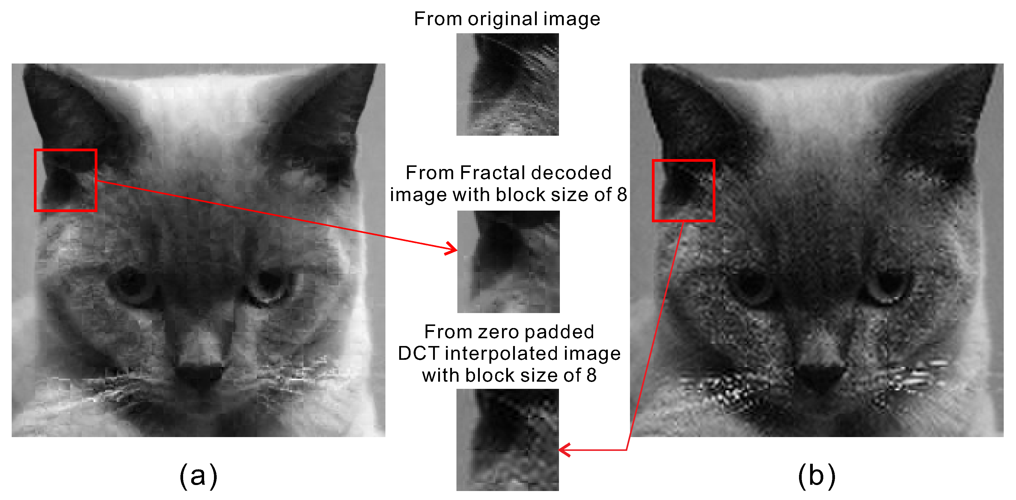
5. Decoding with Interpolation

The main idea of the fractal image interpolation is rather simple. It is based on the assumption that the fractal coding is really a fractal process, and the fractal code’s attractor is a fractal object, such that, by iterating a deterministic transformation on some initial image, a deterministic fractal image will be obtained. The transforms that build the fractal code describes relations between different parts of the image, which is independent from the size and resolution of the image being processed. This means that the image can be decoded to any resolution, higher or lower than that of the original image.
The ability of using a fractal code to interpolate image has been developed in [15,21,22] and is known as “fractal zoom”. It is known as “zoom” because the fractal decoded and enlarged image does not necessarily preserve the pixel intensity correspond to the low-resolution image. In other words, the “zoom” algorithm is not an interpolation algorithm, but a fitting algorithm. For magnification, the range block size κ × κ in the decoded image has to be increased. In particular, for image zooming to double its size, the κ should be doubled.
Finally, although the initial image can be an arbitrary image (in the following, we choose a zero matrix initial image in the following simulation), it has to be the same size as the interpolated image when applied to the PIFS transform. Putting these all together, the fractal zoom-in Cat image of size 512 × 512 obtained from a PIFS encoded 256 × 256 Cat image with κ = 8 is shown in Figure 7. It should be noted that the fractal zooming does not preserve the pixel values and hence performs very bad in traditional objective measures, where PSNR and SSIM are 25.2695 dB and 0.7659, respectively. On the other hand, the fractal zoom-in image performs very good with subjective assessments. Visually, it is vivid that the fractal zoom-in image can provide acute preservation of edges without serration effects and increased brilliance when compared to other image interpolation methods in literature. In summary, the fractal zoom-in image is observed to process the following properties:
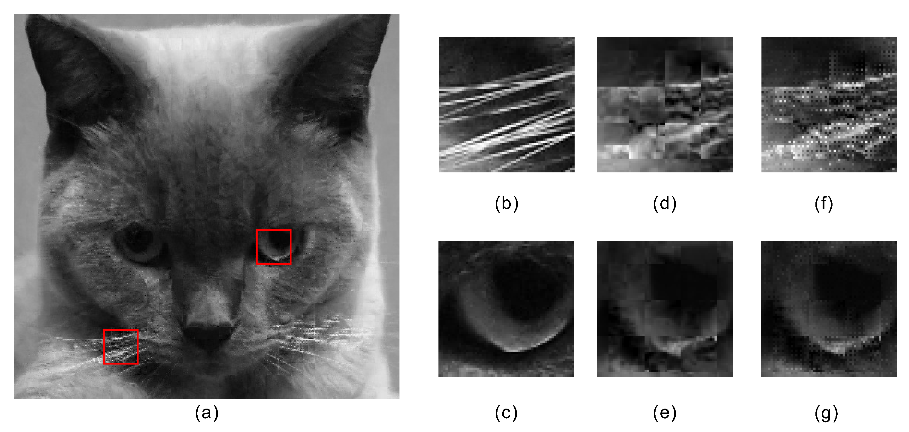
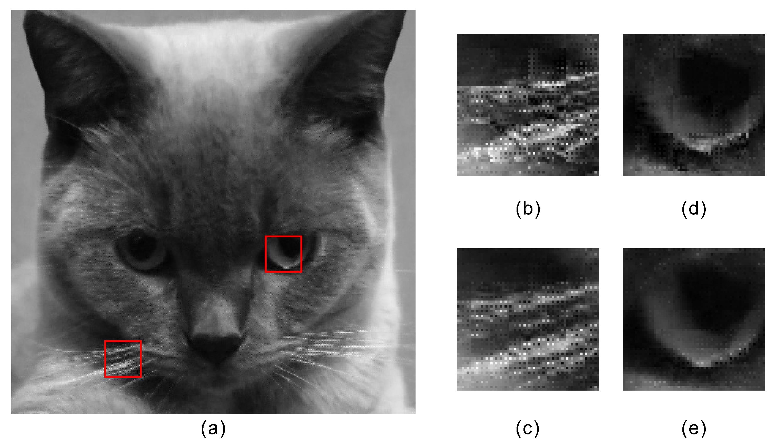
  • When edges are well approximated at the original resolution, they are sharp and fairly well preserved in the interpolated image.
  • Edges do not always match well at block boundaries.
  • The non-fractal blocks are less visually satisfactory, where “notches” are created by non-fractal blocks, which are propagated by iterations onto neighboring blocks.
The loss of details of the non-fractal blocks is mostly caused by the fact that the fractal coding is a lossy process, and the coding error is magnified in the decoding stage during zooming. As a result, a special treatment of this error would be necessary to enable the fractal image interpolation to compete with the classical interpolation methods with respect to objective performance assessments.

From Fitting to Interpolation

Although the PIFS image representation is based on the assumption that the image can be treated as a fractal object, almost all real world images do not satisfy the self-similarity property. The consequence is that the PIFS decoded image will be lossy, and the interpolated image obtained from the application of PIFS cannot guarantee the preservation of the original pixel values. As a result, the traditional fractal zooming can only be considered as fitting instead of interpolation. When that happens, a back propagation algorithm [19] can be employed to recover the original pixel values in the interpolated image. The back propagation obtains a low resolution error image e [ m , n ] by subsampling the fractal zoomed image and subtract the original low resolution image, such that e = g k 2 f . However, as we understand that the fractal decoding depends on the invariant of the affine transformation performed by the fractal encoding process, instead of the underlying image. We have demonstrated this property by initializing the PIFS decoding process with an initial image having all its pixels equal to zero (i.e., a zero matrix), and bilinear interpolated original images, where the fractal decoding algorithm converges to images that are almost exactly the same. As a result, instead of considering the adjustment of the fractal decoded image by iterative fractal interpolation of difference images, we can modify the fractal decoded image in each iteration with an interleave layer, which will enforce all intermediate fractal decoded image to have the same pixel values of f and make it equals f in the corresponding pixel locations. The interleave layer is given by
g k [ p , q ] = f [ m , n ] for p = 2 m and q = 2 n , g k [ p , q ] , otherwise .
The fractal image zooming method will be applied to obtain a high-resolution error image h, such that the corrected high resolution image g k + 1 is given by g k + 1 = g k + h . By iterative application of the back propagation error correction technique a number of times, all pixels in g k are the corresponding pixel of the origin low resolution image f will be able to maintain its intensity. In other words, g k 2 = f , such that all pixels correspond to the original image are replaced by that of the original image in the intermediate decoded interpolated image in each iteration.
Similar algorithms have been considered in [23] where an enhancement layer is introduced in the fractal decoding process within the IFS space. Even though the concept is similar, the enhancement layer considered in [23] cannot guarantee the convergence of the IFS decoding process. On the other hand, the interleave layer introduced in the spatial domain is equivalent to the modification of the contraction transform. Since the underlying transform of the IFS is contractive, the convergence of the system is guaranteed. To show that this method will form a converging IFS, let us consider a downsampling matrix S D with the same size as that of the range block and with element 0 at all the matrix location corresponding to the low-resolution image pixel location, and 1 at all other locations. With the interleave layer, the i-th range block is obtained as
r i = S D P i ( a i d α ( i ) + b i ) + S U f i = P i ( S D a i d α ( i ) + S D b i + S U f i ) = P i ( a ^ i f S D d α ( i ) + b ^ i ) ,
where ⊗ is the Kronecker product, S U is the upsampling matrix with zero padded into the upsampled location, f i is the low-resolution image block with size κ × κ extracted at the corresponding location of the i-th range block in the high-resolution image, furthermore, f = i = 1 N r f i . The lumped matrix b ^ i is thus a constant matrix with respect to the given image f and the fractal code b i . The Kronecker product of a downsampling matrix S D is contractive. As a result, the contractivity of the range block obtained from Equation (18) is guaranteed. The interpolated Cat image achieved by the above IFS with an interleave layer is shown in Figure 8, where it is obvious that the interpolated image has more details and less artifacts than that obtained by Fractal zoom as shown in Figure 7 with improved objective performance where PSNR = 26.41 dB and SSIM = 0.8642, due to the error minimization by back propagation. It should be noted that the proposed pixel replacement scheme does not follow the self-similar property of fractal image representation, which may end up with distinct pixel values (also known as shot noise) to be observed in the interpolated image. Such artifacts will affect the performance of the constructed domain pool for the next iteration, and hence the final image object quality. Furthermore, this pixel replacement procedure in the decoding process does not alter the block processing nature of the PIFS image representation, and hence the interpolated image is still observed to be blocky.

6. Overlapping

Fractal image representation technique is a block based technique and hence blocking artifact is observed to be heavy and considered to be the most important visual artifact in the Fractal decoded image. The blocking artifact is observed to behave like random white noise in nature but is translation variant. In other words, the blocking error depends on where the blocks are extracted from the image to perform the PIFS, and the locations to glue these blocks together. There are a number of ways to ensure the continuity of brightness between blocks. In [2], the means of each range blocks are extracted and the overlaps of the four adjacent blocks are smoothed by a spatial filter with kernel. The smoothing filter assumes translation invariant of the mean brightness across a block boundary, which, however, is not always correct, and might end up blurring the image features when the block boundary co-aligns with the edges of the image features. As a result, instead of considering the translation invariant property of the mean brightness, we shall consider the translation variant property of the blocking artifact random noise, which suggests alleviating the blocking artifacts through averaging interpolated images having different range block boundaries. Such method can be considered as a smoothing filter too. However, this time, the smooth is performed per pixel and hence will not blur the image. Figure 9a shows the “non-shifted”, and Figure 9b,c, d shows the “horizontal shifted”, “vertical shifted”, and “diagonal shifted” images. As a result, the fractal image interpolation results obtained from images that are shifts of one another such that they have different range block boundaries that are averaged to alleviate the discontinuities around the range block boundaries [16,24]. Besides image averaging, overlapping the range block is also able to alleviate the block discontinuities problem [4] to alleviate the block discontinuities. However, range block overlapping is a low-pass filtering operation, which is compared with the median filtering process realized by image averaging, and the median filtering process is more efficient in removing shot noise.
A common selected shift is half of the range block size. The PIFS image coding results of each shifted image will generate one interpolated image. After rectifying the fractal interpolated shifted image (by padding the boundary with the fractal decoded image of the non-shifted image) to be the same size as that obtained from the non-shifted image, all the images will be averaged to produce the final overlapped interpolated image. We shall expect the blocking artifact is alleviated and the image quality is further improved. The interpolated image with overlapping technique is shown in Figure 10a, with the selected zoom-in portions of the cat shown in Figure 10c,e. For comparison, the corresponding zoom-in portions of the Fractal interpolated image without overlap are shown in Figure 10b,d. It can be observed that the blockiness of the interpolated image has largely suppressed, and the details of the texture rich regions of the Cat images can be preserved in the overlapped interpolated image. Besides the blocking artifacts, the shot noise problem due to the interleave layer in Fractal interpolation method with interleaving has also been suppressed. This is because the location of the shot noise pixels are different in fractal decoded images with different shifts. As a result, the averaging action among fractal decoded images with different shot noise pixel locations helps to reduce the shot noise intensity to an HVS non-observable level. The good performance of this image interpolation scheme is also observed in the objective performance measures, where both the PSNR and SSIM are 27.39 dB and 0.887, respectively, which are better than that of other fractal zooming/interpolation methods presented in this paper. This almost perfect fractal image interpolation scheme does come with the very high price of exceptionally high computational complexity and possible high memory requirement.
Recent development of Fractal wavelet image coding/interpolation can help to lower the computational complexity, but the fractal operating on the transform domain (wavelet domain) will lose the nice features of self-similarity in spatial domain, and hence the decoded/interpolated image will no longer look natural, and the edges and features will not be as sharp as traditional fractal image operating in the spatial domain. In view of this quality degradation, the fractal wavelet technique is not discussed in this paper.

7. Conclusions

This paper has shown that fractal image interpolation has the potential to generate high quality interpolated images. One of the major weaknesses of the fractal image interpolation is the use of fixed size range and domain image blocks. There are regions in images that are more difficult to cope with others (such as the eye region of the Cat image), which will require a mechanism to adapt the block size. One of such methods is to use quadtree decomposition. Unfortunately, variable block size fractal image interpolation suffers from huge encoding complexity. Actually, even for range block with uniform size, the search space to be investigated is spanned by the amount of domain block locations, which equals the number of pixels in the image, and the variations of all affine transforms applied to the domain pool generation. Therefore, the key to make fractal image interpolation work is to find methods to reduce the search effort to an acceptable level for real world implementation in everyday home computers. This involves intelligent search methods to be investigated by the readers. In summary, the fractal image interpolation can produce excellent interpolation results for natural images, where very sharp edges can be obtained with almost no ringing artifacts. The con is the very high computational complexity and processing memory requirement, no matter whether it is being applied alone or mixed with various artifacts reduction techniques.
Image interpolation is an ill-posed problem with infinitely many solutions due to the lack of information presented in the low-resolution image. Second, various interpolation techniques and artifact reduction methods can be mixed to achieve better interpolation results. However, mixing different interpolation methods and artifact reduction methods together do not always work, but, when it works, the result will usually be very pleasing. The major fallacies of such mix and match methods will be the increase in computational complexity. Such schemes are usually iterative, which means that the very high computational complexity interpolation algorithm will have to be performed many more times before a prefect interpolated image can be obtained. Therefore, the design of an image interpolation algorithm is to find the best trade-off between the appearance of artifacts (the unfortunate results of a series of wrong assumptions) and the computational complexity.

Author Contributions

Conceptualization, C.W.K. and W.S.T.; Methodology, C.W.K.; Software, C.W.K. and W.S.T.; Validation, C.W.K. and W.S.T.; Formal Analysis, C.W.K.; Investigation, C.W.K. and W.S.T.; Writing—Original Draft Preparation, C.W.K.; Writing—Review and Editing, W.S.T.; Visualization, W.S.T.

Conflicts of Interest

The authors declare no conflict of interest.

Abbreviations

The following abbreviations are used in this manuscript:
IFSIterative Function System
PIFSPartitioned Iterative Function System
PSNRPeak Signal to Noise Ratio
SSIMStructural Similarity
DCTDiscrete Cosine Transform

References

  1. Xu, Y.; Ji, H.; Fermuller, C. Viewpoint invariant texture description using fractal analysis. Int. J. Comput. Vis. 2009, 83, 85–100. [Google Scholar] [CrossRef]
  2. Wee, Y.C.; Shin, H.J. A Novel Fast Fractal Super Resolution Technique. IEEE Trans. Consum. Electron. 2010, 56, 1537–1541. [Google Scholar] [CrossRef]
  3. He, S.H.; Wu, Z. Method of Single Image Super-Resolution Enhancement Based on Fractal Coding. In Proceedings of the 3rd International Confernece on Computer Science and Network Technology, Dalian, China, 12–13 October 2013; pp. 1034–1036. [Google Scholar]
  4. Zhang, Y.; Fan, Q.; Bao, F.; Liu, Y.; Zhang, C. Single-Image Super-Resolution Based on Rational Fractal Interpolation. IEEE Trans. Image Process. 2018, 27, 3782–3797. [Google Scholar] [PubMed]
  5. Xu, H.; Zhai, G.; Yang, X. Single image super-resolution with detail enhancement based on local fractal analysis of gradient. IEEE Trans. Circuits Syst. Video Technol. 2013, 23, 1740–1754. [Google Scholar] [CrossRef]
  6. Chaurasia, V.; Gumasta, R.K.; Kurmi, Y. Fractal Image Compression with Optimized Domain Pool Size. In Proceedings of the International Conference on Innovations in Electronics, Signal Processing and Communication, Shillong, India, 6–7 April 2017; pp. 209–212. [Google Scholar]
  7. Padmashree, S.; Nagapadma, R. Different approaches for implementation of fractal image compression on medical images. In Proceedings of the International Conference on Electrical, Electronics, Communications, Computer and Optimization Techniques, Mysuru, India, 9–10 December 2016; pp. 66–72. [Google Scholar]
  8. Biswas, A.K.; Karmakar, S.; Sharma, S.; Kowar, M.K. Performance of fractal image compression for medical images: A comprehensive literature review. Int. J. Appl. Inf. Syst. 2015, 8, 14–24. [Google Scholar]
  9. Ye, R.; Lan, H.; Wu, Q. A fractal interpolation based image encryption scheme. In Proceedings of the IEEE International Conference on Computer and Communication Engineering Technology, Beijing, China, 18–20 August 2018; pp. 291–295. [Google Scholar]
  10. Liu, M.; Zhao, Y.; Lin, C.; Bai, H.; Yao, C. Resolution-independent up-sampling for depth map using fractal transforms. KSII Trans. Internet Inf. Syst. 2016, 10, 2730–2747. [Google Scholar]
  11. Banach, S. Sur les operations dans les ensembles abstraits et leur application aux equations integrales. Fundam. Math. 1922, 3, 133–181. [Google Scholar] [CrossRef]
  12. Hutchinson, J. Fractals and self-similarity. Indiana Univ. J. Math. 1981, 30, 713–747. [Google Scholar] [CrossRef]
  13. Jacquin, A.E. Image coding based on a fractal theory of iterated contractive image transformations. IEEE Trans. Image Process. 1992, 1, 18–30. [Google Scholar] [CrossRef] [PubMed] [Green Version]
  14. Barnsley, M.F.; Elton, J.H.; Hardin, D.P. Recurrent iterated function systems. Constr. Approx. 1989, 5, 3–31. [Google Scholar] [CrossRef]
  15. Fisher, Y. Fractal Image Compression—Theory and Applications; Springer: New York, NY, USA, 1995. [Google Scholar]
  16. Reusens, E. Overlapped Adaptive Partitioning for Image Coding Based on Theory of Iterated Function systems. In Proceedings of the IEEE Internation Conference on Acoustics, Speech and Signal Processing, Adelaide, SA, Australia, 19–22 April 1994; pp. 569–572. [Google Scholar]
  17. Davoine, F.; Antonini, M.; Chassery, J.M.; Barlaud, M. Fractal image compression based on Delaunay triangulation and vector quantization. IEEE Trans. Image Process. 1996, 5, 338–346. [Google Scholar] [CrossRef] [PubMed]
  18. Reusens, E. Partitioning complexity issue for iterated function system based image coding. In Proceedings of the VII-th European Signal Processing Conference, Edinburg, UK, 13–16 September 1994; pp. 171–174. [Google Scholar]
  19. Kok, C.; Tam, W. Digital Image Interpolation in MATLAB; Wiley-IEEE Press: Hoboken, NJ, USA, 2019. [Google Scholar]
  20. Lu, N. Fractal Imaging; Academic Press: Cambridge, MA, USA, 1997. [Google Scholar]
  21. Gharavi-Al., M.; DeNardo, R.; Tenda, Y.; Huang, T.S. Resolution enhancement of images using fractal coding. In Proceedings of the SPICE Visual Communications and Image Processing, San Jose, CA, USA, 10 January 1997; pp. 1089–1100. [Google Scholar]
  22. Polidori, E.; Dugelay, J.L. Zooming using iterated function systems. Fractals 1997, 5, 111–123. [Google Scholar] [CrossRef]
  23. Chung, K.H.; Fung, Y.H.; Chan, Y.H. Image enlargement using fractal. In Proceedings of the IEEE International Conference on Acoustic, Speech, and Signal Processing, Hong Kong, China, 6–10 April 2003; pp. 273–276. [Google Scholar]
  24. Polidori, E.; Dugelay, J.L. Zooming using iterated function systems. In Proceedings of the NATO ASI on Image Encoding and Analysis, Trondheim, Norway, 8–17 July 1995. [Google Scholar]
Figure 1. The original image of the Cat and the partitioned images with edge overlaying the partitions by three different range block partition methods: (a) original image; (b) partitioned image by uniform partition; (c) partitioned image by uniform partition quadtree partition; and (d) partitioned image by HV partition.
Fractalfract 03 00007 g001
Figure 2. Fractal encoding by matching range blocks with grayscale transformed domain blocks from the domain pool.
Fractalfract 03 00007 g002
Figure 3. Cat image of size 256 × 256 encoded with 8 × 8 range block fractal and decoded under different iterations an initial image of a zero matrix: (a) the 3rd iteration; (b) the 5th iteration; (c) the 7th iteration; and (d) the 20th iteration.
Fractalfract 03 00007 g003
Figure 4. Comparison of Cat image of size 256 × 256 by (a) fractal decoding with 20 iterations and (b) zero padded DCT interpolation with only the low frequency 4 × 4 DCT coefficients block being retained, where the same block size of 8 × 8 is adopted in both methods.
Fractalfract 03 00007 g004
Figure 5. Comparison of Fractal decoded Cat image of size 256 × 256 obtained from the same fractal codebook but with different initial images at the 20th iteration, where the same block size of 8 × 8 is applied in the decoding: (a) a zero matrix as an initial image and (b) the original Cat image as initial image, where both the decoded images have the same PSNR and SSIM at 26.54 dB and 0.726, respectively.
Fractalfract 03 00007 g005
Figure 6. Cat image of size 256 × 256 with 8 × 8 range block fractal encoding and (a) decoded with 8 × 8 range block size at the 20th iterations, and the associated zoom-in image block of the eye of the Cat in (b) the same image decoded with 4 × 4 range block size at the 30th iterations, where a zero matrix initial image are adopted in both decoding processes.
Fractalfract 03 00007 g006
Figure 7. Fractal zoom-in Cat image in (a) the same size as that of original image (i.e., 256 × 256 ) and (b) an enlargement to the size of 512 × 512 , with both images decoded with identical range block size of 8 × 8 , zero image as initial image, and the number of iterations of 20 (PSNR = 25.2695 dB, SSIM = 0.7659).
Fractalfract 03 00007 g007
Figure 8. Fractal interpolated Cat image by a factor of 2 to 512 × 512 at the 15th iteration with range block size of 8 × 8 interleaved with low-resolution Cat image pixel layer (PSNR = 26.41 dB, SSIM = 0.8542): (a) the full interpolated image; zoom-in portion of the whiskers of (b) the original Cat image, (d) the interpolated image by fractal decoding with κ = 16 × 16 , and (f) the interpolated image by fractal interpolation with interleaving; zoom-in portion of the eye of (c) the original Cat image, (e) the interpolated image by fractal decoding with κ = 16 × 16 , and (g) the interpolated image by fractal interpolation with interleaving.
Fractalfract 03 00007 g008
Figure 9. Illustration of different block partition methods: (a) the original “non-shifted” image f; (b) the “horizontal shifted” image F 1 ; (c) the “vertical shifted” image F 2 ; and (d) the “diagonal shifted” image F 3 .
Fractalfract 03 00007 g009
Figure 10. A 2 × interpolated Cat image by mean filtering a set of four cyclic spin fractal decoding images (original plus 3 other shifted images) with doubled range block size (i.e., 16 × 16 ) and interleaved low-resolution image pixels using fractal interpolation method with interleaving (PSNR = 27.39 dB, SSIM = 0.887): (a) the full interpolated image; (b) zoom-in portion of the whiskers of the Cat image obtained from fractal interpolation method with interleaving but nomean filtering (same as Figure 8f), and (c) from mean filtering shifted fractal decoded images; (d) zoom-in portion of the eye of the Cat image obtained from a fractal interpolation method with interleaving but no mean filtering (the same as Figure 8g), and (e) from mean filtering shifted fractal decoded images.
Fractalfract 03 00007 g010
Table 1. Approximation of 5 by Newton’s method.
n x n x n x n
0125
13.0000002.2500002.625000
22.3333332.2361112.264881
32.2380952.2360682.236251
42.2360692.2360682.236068
52.2360682.2360682.236068
62.2360682.2360682.236068
Table 2. Fractal image representation of the 256 × 256 Cat image with range block size of 4 × 4 and 8 × 8 , respectively, with fractal encoder running in MATLAB R2016b on an MS Windows 7 PC with Quad Core Xeon E5520 @ 2.27 GHz and 8 GB RAM. The fractal domain pool is computed with the pixel location of the top left hand corner of the matched domain block being stored as 8-bit data. Furthermore, each component in the scalar transform ( a , b ) is quantized to 16-bit data.
Block Size 4 × 4 8 × 8
Time to Encode15 min3 min
Size of pool16 × 62,001 double64×58,081 double
Fractal Code Size0.375 byte/pixel0.07 byte/pixel
Table 3. 256 × 256 Cat image reconstructed from fractal image representation using range block size of 4 × 4 and 8 × 8 , respectively, with the decoding process begins with a zero matrix initial reference image running in MATLAB R2016b on MS Windows 7 PC with Quad Core Xeon E5520 @ 2.27GHz and 8 GB RAM.
Block Size 4 × 4 Double 8 × 8 Double
Size of pool16 × 62,001 double64 × 58,081 double
No of Iterations3020
Time to decode50 mins5 mins
PSNR30.9964 dB26.5392 dB

