On the Fractal Langevin Equation


Abstract
:1. Introduction
2. Basic Tools
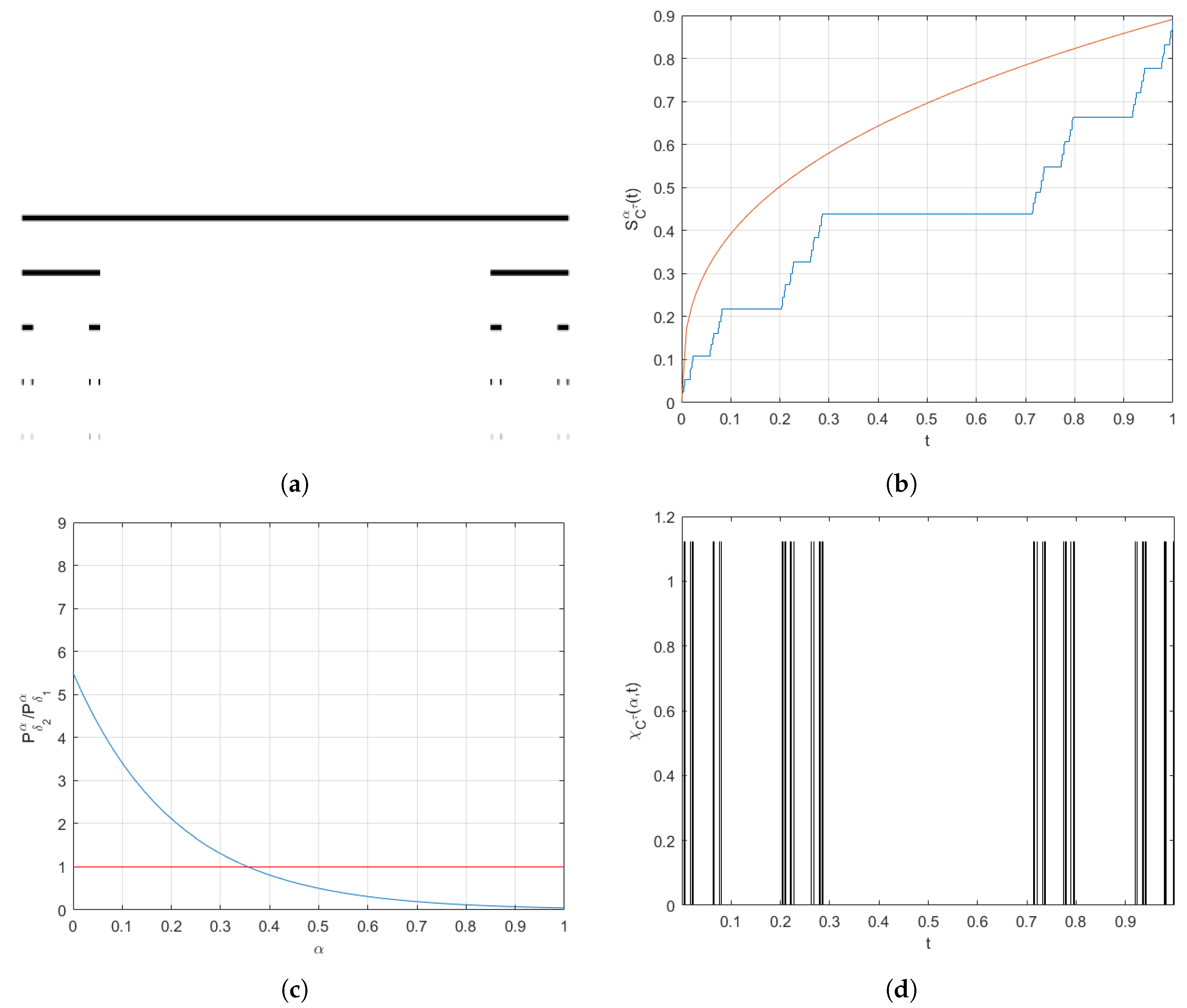
2.1. Middle- Cantor Set
- (I)
- Delete an open interval of length from the middle of the .
- (II)
- Remove disjoint open intervals of length from the remaining sections of step I.
- (III)
- Pick up disjoint open intervals of length from the remaining sections of previous step, and so on ad infinitum.
2.2. Local Fractal Calculus
3. Fractal Langevin Equation with Different Coefficients
3.1. Fractal Over-Damped Langevin Equation
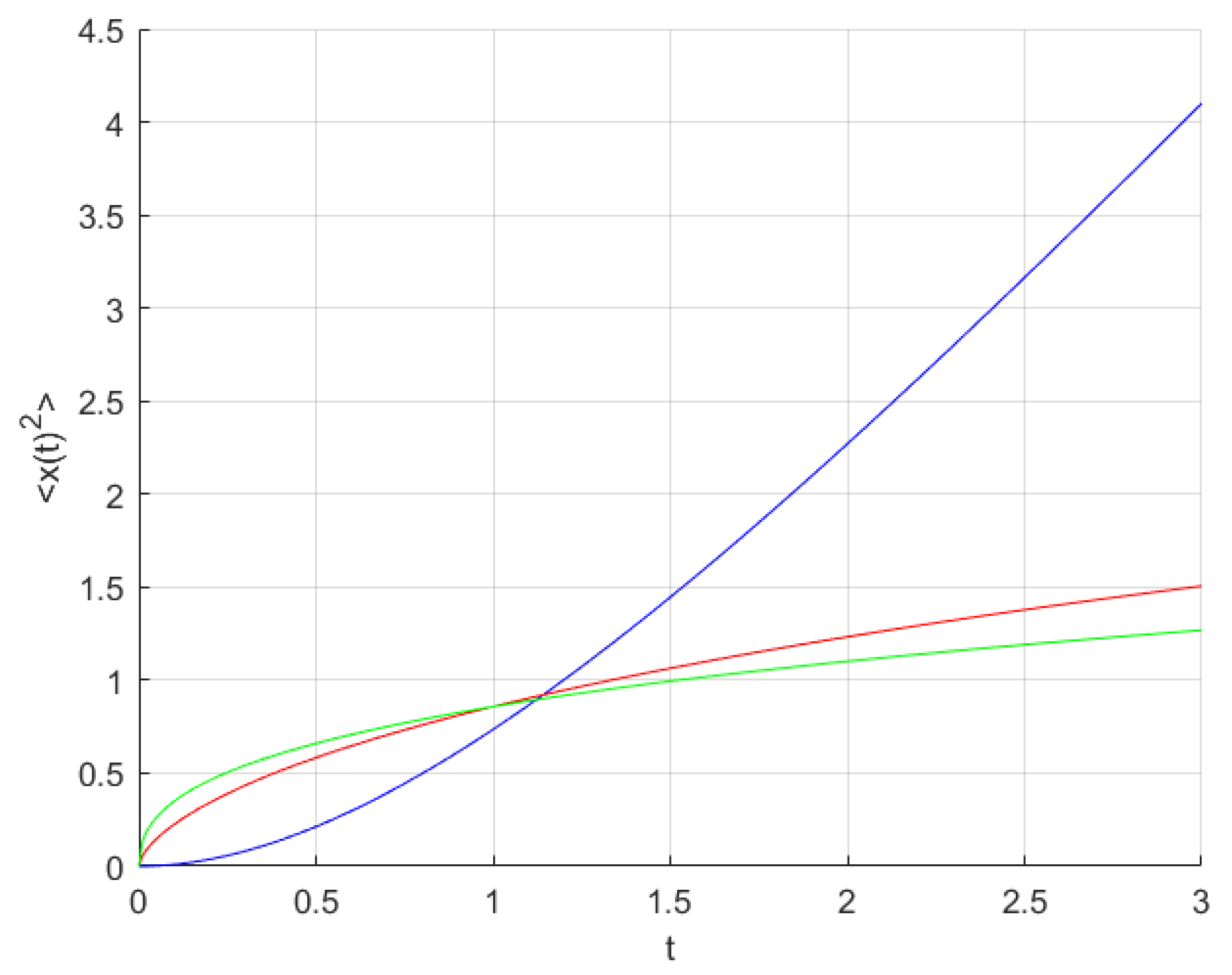
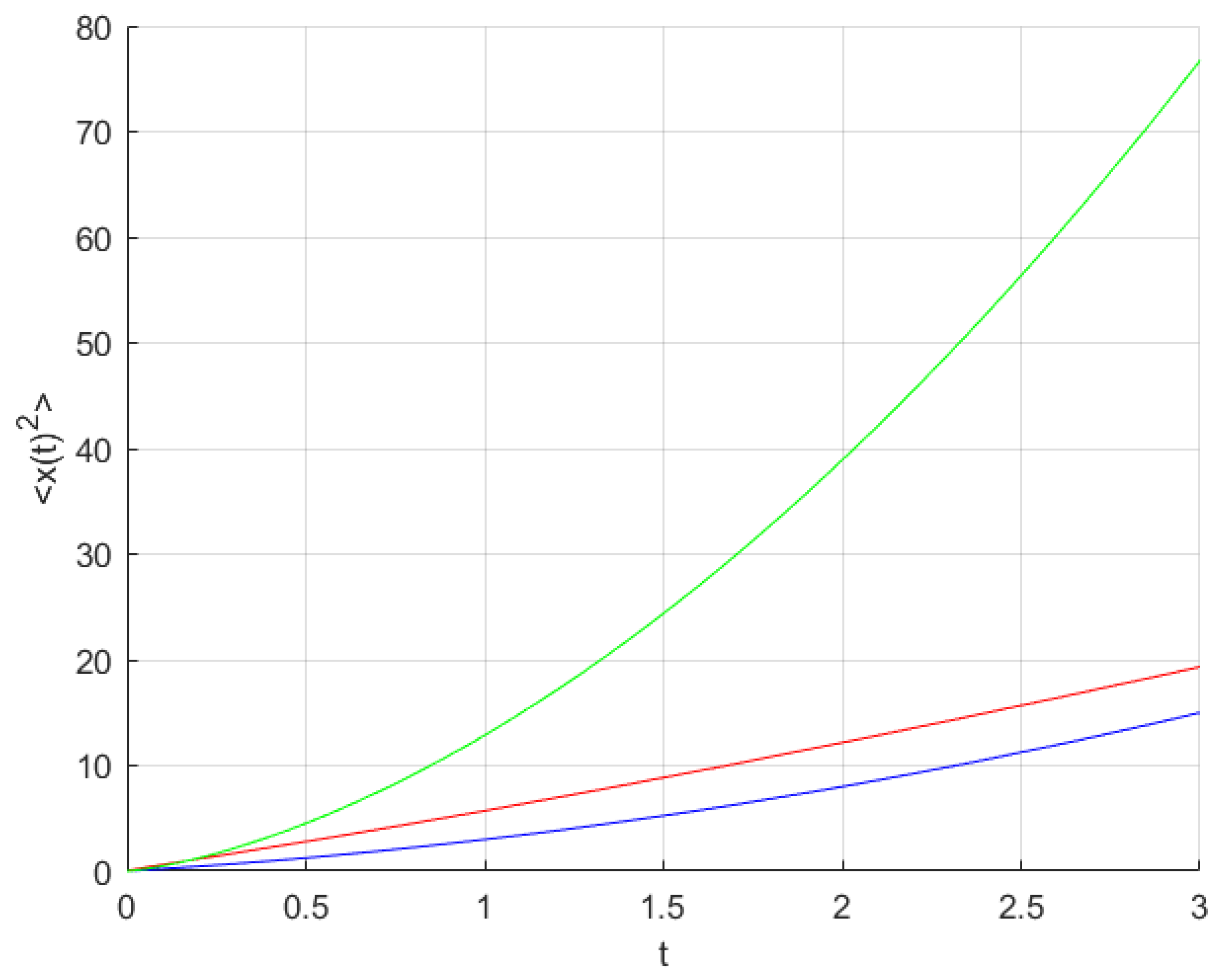
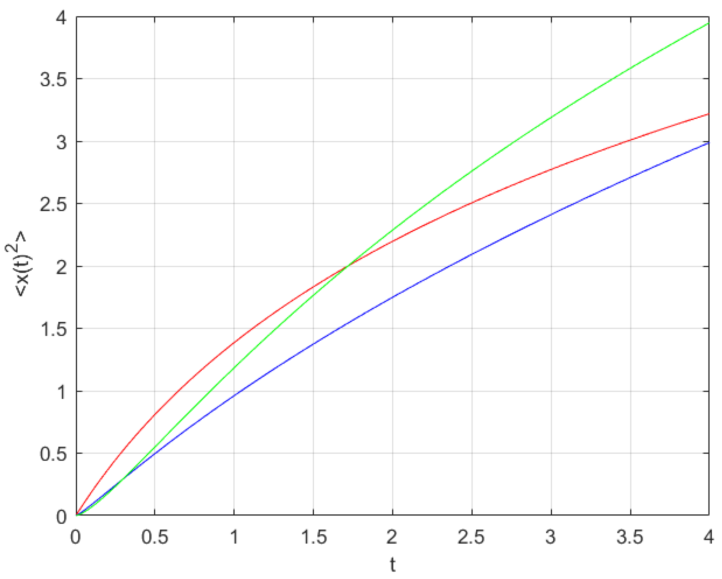
3.2. Fractal Under-Damped Langevin Equation
4. Fractal Scaled Brownian Motion
5. Conclusions
Funding
Conflicts of Interest
References
- Mandelbrot, B.B. The Fractal Geometry of Nature; WH Freeman: New York, NY, USA, 1983; Volumn 173. [Google Scholar]
- Kigami, J. Analysis on Fractals; Cambridge University Press: Cambridge, UK, 2001. [Google Scholar]
- Falconer, K. Techniques in Fractal Geometry; John Wiley and Sons: Hoboken, NJ, USA, 1997. [Google Scholar]
- Freiberg, U.; Zahle, M. Harmonic calculus on fractals-a measure geometric approach I. Potential Anal. 2002, 16, 265–277. [Google Scholar] [CrossRef]
- Strichartz, R.S. Differential Equations on Fractals: A Tutorial; Princeton University Press: Princeton, NJ, USA, 2006. [Google Scholar]
- Cattani, C. Fractals and hidden symmetries in DNA. Math. Probl. Eng. 2010, 2010, 507056. [Google Scholar] [CrossRef]
- Cattani, C. Fractional Calculus and Shannon Wavelet. Math. Probl. Eng. 2012, 2012, 502812. [Google Scholar] [CrossRef]
- Rodriguez-Vallejo, M.; Montagud, D.; Monsoriu, J.A.; Ferrando, V.; Furlan, W.D. Relative Peripheral Myopia Induced by Fractal Contact Lenses. Curr. Eye Res. 2018, 43, 1514–1521. [Google Scholar] [CrossRef] [PubMed]
- Barlow, M.T.; Perkins, E.A. Brownian motion on the Sierpinski gasket. Probab. Theory Relat. Fields 1988, 79, 543–623. [Google Scholar] [CrossRef]
- Balankin, A.S. A continuum framework for mechanics of fractal materials I: From fractional space to continuum with fractal metric. Eur. Phys. J. B 2015, 88, 90. [Google Scholar] [CrossRef]
- Zubair, M.; Mughal, M.J.; Naqvi, Q.A. Electromagnetic Fields and Waves in Fractional Dimensional Space; Springer: New York, NY, USA, 2012. [Google Scholar]
- Nottale, L.; Schneider, J. Fractals and nonstandard analysis. J. Math. Phys. 1998, 25, 1296–1300. [Google Scholar] [CrossRef]
- Célérier, M.N.; Nottale, L. Quantum-classical transition in scale relativity. J. Phys. A Math. Gen. 2004, 37, 931–955. [Google Scholar] [CrossRef]
- Kolwankar, K.M.; Gangal, A.D. Local fractional Fokker–Planck equation. Phys. Rev. Lett. 1998, 80, 214. [Google Scholar] [CrossRef]
- El-Nabulsi, R.A. Path integral formulation of fractionally perturbed Lagrangian oscillators on fractal. J. Stat. Phys. 2018, 172, 1617–1640. [Google Scholar] [CrossRef]
- Das, S. Functional Fractional Calculus; Springer Science Business Media: Berlin, Germany, 2011. [Google Scholar]
- Podlubny, I. Fractional Differential Equations; Academic Press: New York, NY, USA, 1999. [Google Scholar]
- Chen, W.; Sun, H.-G.; Zhang, X.; Koroak, D. Anomalous diffusion modeling by fractal and fractional derivatives. Comput. Math. Appl. 2010, 59, 1754–1758. [Google Scholar] [CrossRef]
- Sumelka, W.; Voyiadjis, G.Z. A hyperelastic fractional damage material model with memory. Int. J. Solids Struct. 2017, 124, 151–160. [Google Scholar] [CrossRef]
- Parvate, A.; Gangal, A.D. Calculus on fractal subsets of real-line I: Formulation. Fractals 2009, 17, 53–148. [Google Scholar] [CrossRef]
- Parvate, A.; Gangal, A.D. Calculus on fractal subsets of real line II: Conjugacy with ordinary calculus. Fractals 2011, 19, 271–290. [Google Scholar] [CrossRef]
- Satin, S.; Gangal, A.D. Langevin Equation on Fractal Curves. Fractals 2016, 24, 1650028. [Google Scholar] [CrossRef]
- Golmankhaneh, A.K.; Fernandez, A.; Baleanu, D. Diffusion on middle-ξ Cantor sets. Entropy 2018, 20, 504. [Google Scholar] [CrossRef]
- Golmankhaneh, A.K.; Fernandez, A. Fractal Calculus of Functions on Cantor Tartan Spaces. Fractal Fract 2018, 2, 30. [Google Scholar] [CrossRef]
- Golmankhaneh, A.K.; Balankin, A.S. Sub-and super-diffusion on Cantor sets: Beyond the paradox. Phys. Lett. A 2018, 382, 960–967. [Google Scholar] [CrossRef]
- Bodrova, A.S.; Chechkin, A.V.; Cherstvy, A.G.; Safdari, H.; Sokolov, I.M.; Metzler, R. Underdamped scaled Brownian motion: (Non-)existence of the overdamped limit in anomalous diffusion. Sci. Rep. 2016, 6, 30520. [Google Scholar] [CrossRef] [PubMed]
- Robert, D.; Urbina, W. On Cantor-like sets and Cantor-Lebesgue singular functions. arXiv, 2014; arXiv:1403.6554. [Google Scholar]


© 2019 by the author. Licensee MDPI, Basel, Switzerland. This article is an open access article distributed under the terms and conditions of the Creative Commons Attribution (CC BY) license (http://creativecommons.org/licenses/by/4.0/).
Share and Cite
Khalili Golmankhaneh, A. On the Fractal Langevin Equation. Fractal Fract. 2019, 3, 11. https://doi.org/10.3390/fractalfract3010011
Khalili Golmankhaneh A. On the Fractal Langevin Equation. Fractal and Fractional. 2019; 3(1):11. https://doi.org/10.3390/fractalfract3010011
Chicago/Turabian StyleKhalili Golmankhaneh, Alireza. 2019. "On the Fractal Langevin Equation" Fractal and Fractional 3, no. 1: 11. https://doi.org/10.3390/fractalfract3010011
APA StyleKhalili Golmankhaneh, A. (2019). On the Fractal Langevin Equation. Fractal and Fractional, 3(1), 11. https://doi.org/10.3390/fractalfract3010011