Article

Identifying the Fractional Orders in Anomalous Diffusion Models from Real Data

1
Department of Mathematics and Physics, Roma Tre University, 1, Largo S. Leonardo Murialdo, 00146 Rome, Italy
2
Faculty of Engineering, International Telematic University UNINETTUNO, 00186 Rome, Italy
3
Institute for the Applications of Computing, Italian National Research Council, 00185 Rome, Italy
*
Author to whom correspondence should be addressed.
Fractal Fract. 2018, 2(1), 14; https://doi.org/10.3390/fractalfract2010014
Submission received: 10 October 2017 / Revised: 8 February 2018 / Accepted: 15 February 2018 / Published: 24 February 2018
(This article belongs to the Special Issue Fractional Dynamics)

Abstract

:
An attempt is made to identify the orders of the fractional derivatives in a simple anomalous diffusion model, starting from real data. We consider experimental data taken at the Columbus Air Force Base in Mississippi. Using as a model a one-dimensional fractional diffusion equation in both space and time, we fit the data by choosing several values of the fractional orders and computing the infinite-norm “errors”, representing the discrepancy between the numerical solution to the model equation and the experimental data. Data were also filtered before being used, to see possible improvements. The minimal discrepancy is attained correspondingly to a fractional order in time around 0 . 6 and a fractional order in space near 2. These results may describe well the memory properties of the porous medium that can be observed.

1. Introduction

In this paper, we provide some justification of the widespread use of simple linear parabolic fractional partial differential equations (fPDEs) to model a number of physical phenomena, such as, for instance, diffusion of fluids in porous media [1] and in particular fluid flow of tracers through porous media. We do that by identifying the fractional orders of the aforementioned fPDE from experimental data.
Several laboratory experiments have been performed concerning one-dimensional flows, to determine the flow rate through uniformly packed columns filled in by certain porous media, where a constant pressure was applied to the lower boundary, see [2,3]. These measurements were done using diffusivity meters. The experimental setup was designed aiming at determining the memory properties of the observed dynamical behavior. The latter could be considered as an anomalous diffusion, and was well reproduced by a suitable fPDE modeling of the constitutive laws involving pressure gradient–flux and pressure–density variations. In such experiments, one may use water as fluid and a variety of porous media. Clearly, one of the key-factors was the size (or better, the size distribution) of the specific medium’s grains. In the laboratory experiments of [2,3], special attention was paid to detect memory effects, experimentally identifying the fractional orders in time in the aforementioned constitutive equations.
On the theoretical side, there are works in the literature on several kinds of inverse problems for fractional differential equations [4,5,6,7], but very little attention seems to have been devoted to determining the fractional orders. We can mention two papers by Bondarenko and Ivaschenko, concerning only some special problems for time fractional diffusion equations [8,9], and the recent contribution in [10] where the focus is on identifying the order in simple fractional ordinary differential equations, exploiting asymptotics and special (Mittag-Leffler) functions. See also [11,12].
In this paper, in contrast to what was done in [2,3], we compare certain real, i.e., experimental data taken at the Columbus Air Force Base in Mississippi, USA [13,14], with those provided by the numerical solution of a certain fPDE, by varying both fractional orders in time and in space, assessing the mismatch for certain fixed values of the orders of fractional derivatives as well as of the initial conditions. The real data we used here refer to the MADE-2 experiment, where some tritium concentration was injected, representing contaminant transport in a highly heterogeneous aquifer [13,14]. In such papers, the 1D data were actually obtained by suitably processing typical 2D or 3D concentration data sets. This concentration depends, in general, on both time and place (measured in days and meters, respectively). We considered three fixed times of observation, when they were obtained. Our approach can be considered in the spirit of the modern attitude of “learning from data”, in such a way to infer the governing equations of the physical model, as put forth at the present time by machine learning techniques, within the modern Data Science [15]. However, the idea here is grounded on basic physical principles.
Here is the plan of the paper. In Section 2, we state the problem with some emphasis on the numerical method we adopted, in Section 3 we describe the discretization method used to solve numerically the model equation, and in Section 4 we illustrate our method through some numerical examples. Conclusions and future developments are given in a final section, at the end of the paper.

2. Statement of the Problem

Consider the one-dimensional anomalous diffusion equation, fractional in both, space and time,
0 D t γ u = a α u | x | α + f ( x , t ) ,
where u = u ( x , t ) represents some mass concentration (of tritium), 0 D t γ u is the Caputo fractional derivative in time of u, α u | x | α is the Riemann-Liouville fractional derivative in space of u, a > 0 , 0 < γ 1 , 1 < α 2 , x [ x ̲ , x ¯ ] , t [ 0 , T ] , for some x ̲ , x ¯ , T > 0 , along with the boundary conditions u ( x ̲ , t ) = u 1 , u ( x ¯ , t ) = u 2 , and the initial condition u ( x , 0 ) = u 0 ( x ) , for some constants u 1 , u 2 , and some u 0 ( x ) , while f ( x , t ) is a certain external source (if any).
We solved such a problem numerically using finite differences of the kind of Grünwald-Letnikov (GL) for our approximations [16]. We started considering a mesh in the space-time domain [ x ̲ , x ¯ ] × [ 0 , T ] , denoting with u j n the numerical approximation of the solution at the mesh points, ( x j , t n ) , i.e., u j n : = u ( x j , t n ) . We then replaced the continuous fractional derivatives operators, in both, time and space, in Equation (1), with their GL approximation. We thus obtain a difference equation whose solution ( u j n ) will provide estimated values of the exact solution, u ( x , t ) , at the mesh points.
For a given fractional differential operator, there are several possible forms of difference operators, and hence there are several different finite difference methods capable to solve our problem.
We should recall, at this point, that many authors have already considered similar problems, but most often adopting a fractional order only either in time or in space, see, e.g., [17,18,19,20]. When fluid flow through porous media is studied, usually, only fractional derivatives in time were considered.
Here we take a uniform spatial step-size, Δ x : = x i + 1 - x i , and consider the space fractional differential operator in the sense of Riemann-Liouville, that we will approximate by means of “GL differences”. Fractional time derivatives in the sense of Caputo will be discretized again by GL differences, with a constant time step-size, Δ t : = t n + 1 - t n .
We thus obtain a finite difference algorithm, ending up with a linear system like
U n + 1 = ( A - S ) U n ,
where
U n : = ( u 1 n , u 2 n , , u M n ) T ,
and A and S represent the discretized time and space operators (two matrices), respectively, obtained through the GL discretization, see [16].
A code was then written to compute U n , by minimizing, at each time step, the norms (with respect to space) of the discrepancies between the experimental and the numerically computed values obtained by solving (numerically) the aforementioned anomalous diffusion equation. We will denote with v j n the experimental data, measured in the field, and with
V n : = ( v 1 n , v 2 n , , v M n ) T ,
the vector of the measured data.
Relatively recently, in [2], experimental results have been obtained to estimate the physical parameters governing the dynamical behavior of the flow of tracers through a certain given porous medium, in particular to observe the aforementioned memory effects described by parameters such as, for instance, the order of the fractional derivative with respect to time. Memory effects may also be due to the size of the tank containing the porous medium in the laboratory, the particle size distribution, the stability of the initial particle distribution.
The function to minimize is then the error, i.e., the discrepancy between the numerically computed value, U n , and the value of u ( x , t ) obtained by using the real experimental data, V n , that is U n - V n .

3. Discretization of Partial Derivatives in Time and Space

Let us consider the nodes ( j Δ x , n Δ t ) , for a given fixed j, j { 1 , 2 , , M } , n = 0 , 1 , 2 , , N , corresponding to all time levels at the j-th space discretization node. Then, the approximation scheme can be represented through a matrix that we will call B N γ [16], so that we can write
u j , N γ u j , N - 1 γ . . . u j , 2 γ u j , 1 γ u j , 0 γ T = B N γ u j , N u j , N - 1 . . . u j , 2 u j , 1 u j , 0 T ,
where u j , n γ represents the numerical approximation of the time derivative of order γ at the ( j , n ) node of the mesh.
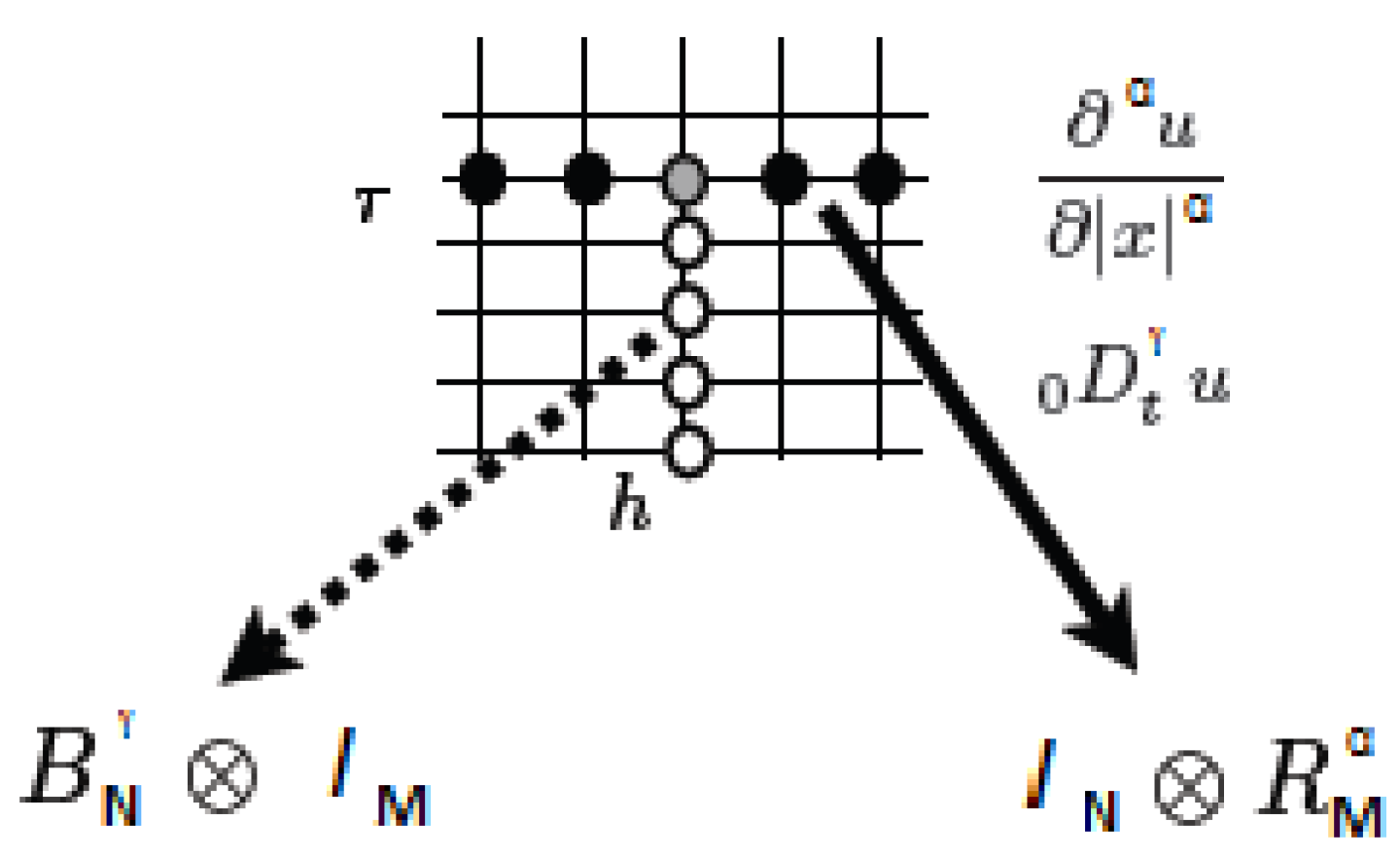
In order to obtain a simultaneous approximation of the time derivative of order γ and space derivatives of order α of u ( x , t ) , at each grid point shown in Figure 1, we rearrange all function values, u j n , at the discretization nodes, in a column vector,
u M N : = u M N u M - 1 N u 1 N u 0 N ; u M N - 1 u M - 1 N - 1 u 1 N - 1 u 0 N - 1 ;
; u M 1 u M - 1 1 u 1 1 u 0 1 ; u M 0 u M - 1 0 u 1 0 u 0 0 T .
We can arrange all the numerical values of the solution in a matrix, which contains the numerical results of every discretized value of time and space. Such a matrix represents the iteration matrix which yields the discretization vector U t γ of the fractional partial derivative of order γ with respect to time, and can be written as the Kronecker product of the matrix B N γ , corresponding to the fractional ordinary derivative of order γ , and the identity matrix, I M ,
T M N γ = B N γ I M ,
see [16]. Recall that here N is the number of time steps and M is the number of space discretization nodes. The corresponding stencil is depicted in Figure 1.
Similarly, the matrix governing the transformation of the vector U n into the vector U x α of the fractional partial space derivative of order α can be obtained as the Kronecker product of the unit matrix I N (where N is the number of the time steps) in the mesh. The matrix R N α , which corresponds to a derivative of order α [21,22] is given by
S M N γ = I N R M α .
All this is illustrated in Figure 1, where the nodes in black and gray (corresponding to all discretization nodes, from the leftmost to the rightmost nodes) are used to approximate the fractional-order derivative at the node in gray.
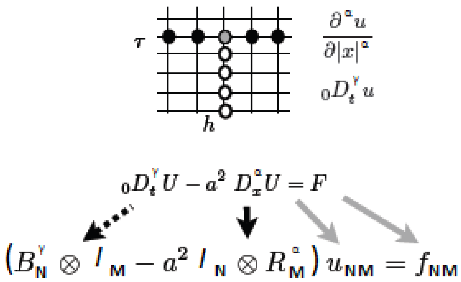
With these approximations for the fractional partial derivatives made with respect to both variables, we can discretize at once the fractional diffusion equation in (1) (see Figure 2), that is
0 D t γ u = a α u | x | α ,
without any forcing term, obtaining
B M γ I N - a I M R N α u M N = 0 .
Note that the system’s matrix is banded upper triangular.
In closing this section, we observe the following. There are currently in the literature still unclear issues concerning imposing local boundary values to nonlocal differential equations such as fPDEs, see, e.g., [23]. When the domain is bounded, in many cases it seems reasonable to extend the Dirichlet data to all space, outside the domain. Here we will adopt this strategy.

4. Numerical Examples

In this section, we present some numerical examples, where we show that the identification of both fractional orders of derivative, in space and time, can be accomplished, from the knowledge of the available real data. We attempt to model a certain real phenomenon either taking into account a possible source term or not. The real data were also filtered prior to using them.

4.1. Example 1

Consider the one-dimensional fractional diffusion equation
0 D t γ u = a α u | x | α , ( x , t ) ( 0 , 1 ) × ( 0 , T ] ,
characterized by fractional derivatives in both, space and time (measured in meters and days, respectively), satisfied by the mass concentration of tritium, u = u ( x , t ) , measured in picoCuries per milliliter, with a = 10 - 5 , 0 < γ 1 , 1 < α 2 , T = 328 , under the homogeneous boundary conditions u ( 0 , t ) = u ( 1 , t ) = 0 (that will be extended to the entire real line), and the initial condition u 0 ( x ) : = x ( 1 - x ) . Some values for a can be found in the literature, often much smaller than the value we used here [24,
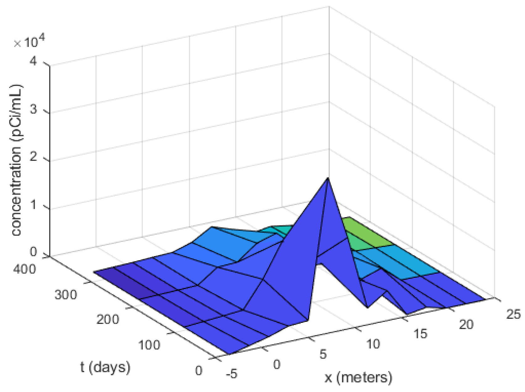
25], but the value we used seemed to be more appropriate in the present case as a modeling choice. Both, the initial profile and the homogeneous boundary values are inferred by inspecting the available real data. The values of 
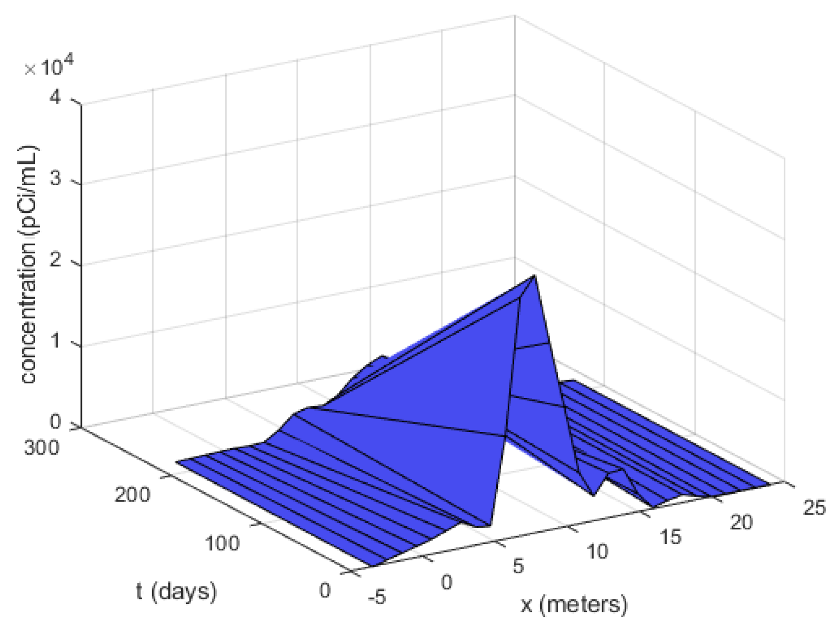
u, obtained solving numerically the problem in (15) should be compared with the experimental data, see Figure 3. Such data come from tests made at the Columbus Air Force Base in Mississippi, see [13,14]. We fitted them against the results of the numerical integration of Equation (15) (i.e., the numerically approximated values u j n of u ( x , t ) ), for several values of the parameters involved in the model. All data have been normalized to the spatial range [ 0 , 1 ] , by dividing by their largest value.
In Table 1, Table 2 and Table 3 below, the discrepancies between the numerical solution and the experimental data are shown, for several chosen values of γ and α . The notation 1 . 1 ( 0 . 1 ) 2 . 0 means taking all values between 1 . 1 and 2 . 0 at steps of size 0 . 1 , that is considering all values 1 . 1 , 1 . 2 , 1 . 3 , , 1 . 9 . In all tables, M = 14 is the number of points of the space-grid, and N = 328 is that of time steps. In Figure 4, the error versus α and γ is plotted in log scale.
Inspecting these tables, we can see that, in general, the best results are achieved for α = 2 . 0 , and, more precisely, correspondingly to the pair ( γ , α ) = ( 0 . 6 , 2 . 0 ) , we obtained
U n - V n = 0 . 0030 .
We now apply to the experimental data a filter based on a wavelet decomposition of data, see [26]. In Figure 5, we show the filtered data. We used the filter wavedec of MATLAB [27].
Now the best results are obtained correspondingly to the values ( γ , α ) = ( 0 . 6 , 1 . 9 ) , see Table 4. The slightly smaller discrepancy is on the third decimal digit, having now
U n - V n 0 . 0026 .
In particular, when α = 2 and γ = 1 (that is, in the case of classical diffusion), larger errors, at least three times larger in the infinite norm, are obtained. The best results are obtained for α = 2 (classical Laplacian), but with a time fractional derivative of order γ = 0 . 6 , that is, appreciably smaller than 1. In this case, we obtain the discrepancy
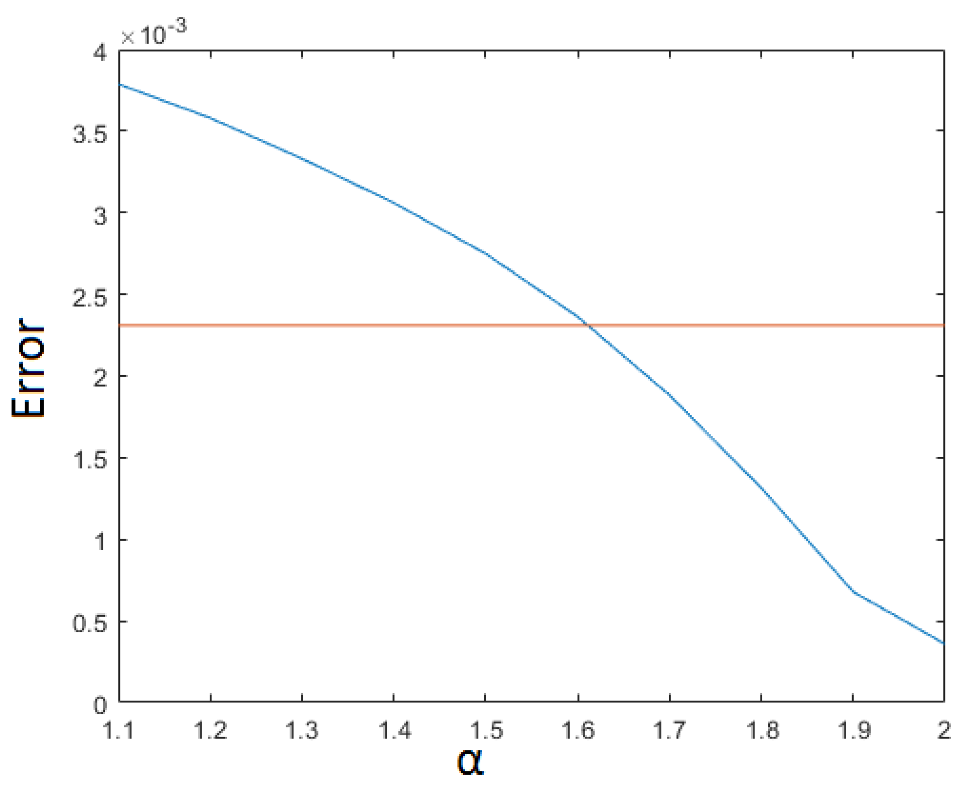
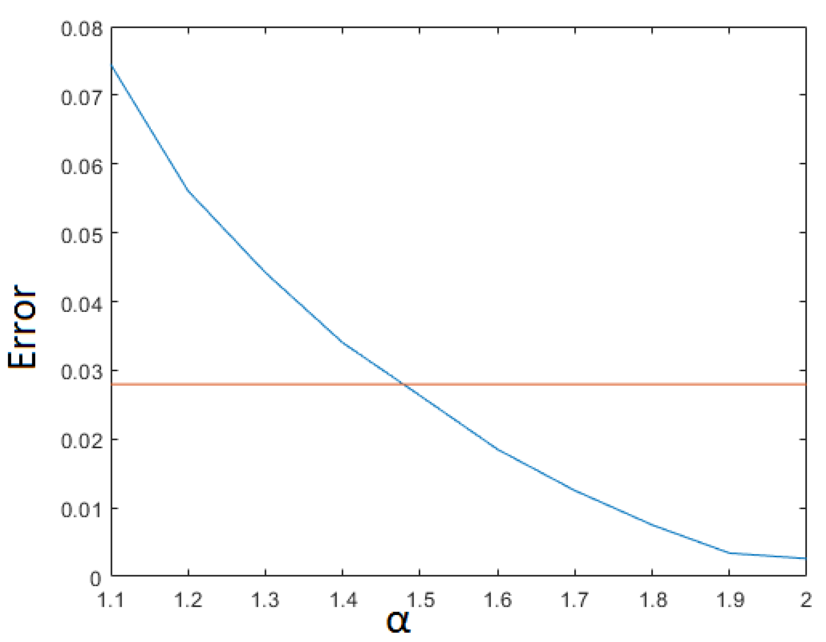
U n - V n 0 . 0026 .
In Figure 6 the error is plotted as a function of α for some fixed value of γ .

4.2. Example 2

Consider the one-dimensional fractional diffusion equation
0 D t γ u = a α u | x | α + δ ( x - 0 . 5 ) δ ( t ) , ( x , t ) ( 0 , 1 ) × ( 0 , T ] ,
fractional in both, space and time, satisfied by the tritium concentration, u = u ( x , t ) , with a = 10 - 5 , 0 < γ 1 , 1 < α 2 , T = 328 , under the homogeneous boundary conditions u ( 0 , t ) = u ( 1 , t ) = 0 (that will be extended to the entire real line), and the initial condition u ( x , 0 ) : = u 0 ( x ) 0 . Here δ are the delta functions. Indeed, introducing such a forcing term should more realistically account for describing a source located initially in the middle of the space domain; see the experimental data in Figure 3. Better results are in fact obtained doing so.
In the numerical simulations, the delta functions on the right-hand side of (15) have been implemented using suitable gaussian functions. We chose the gaussian functions e x p ( - ( x - 0 . 5 ) 2 2 · 0 . 025 2 ) , and e x p ( - t 2 2 · 0 . 025 2 ) . We were interested in using peaked functions but with a prescribed maximum value, i.e., the value 1, in view of the data normalization.
In Table 5, Table 6 and Table 7 below, we show the discrepancies between the numerical solution and the experimental data, for several values that we chose for γ and α .
We can see that, again, the best results are achieved for ( γ , α ) = ( 0 . 6 , 2 . 0 ) . Using as before N = 328 and M = 14 , we obtained about
U n - V n 0 . 000201 ,
which is appreciably smaller than that of Example 1. Note however that having a smaller value for the minimal discrepancy is only meaningful in view of a reliable identification of the optimal parameter γ and α . In fact, different data coming from the same experiments will provide, in general, different discrepancy. What matters is that again the same values for γ and α 
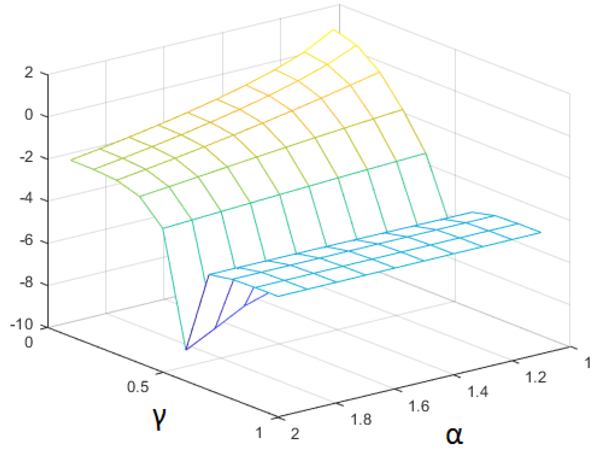
have been inferred. An error surface is shown, as a function of α and γ in Figure 7.
Applying the filter to the experimental data, as before, the best results were obtained correspondingly to the values ( γ , α ) = ( 0 . 6 , 2 . 0 ) , see Table 8. The results in (16) and in (12) differ on the third digit.
When α = 2 and γ = 1 (classical diffusion), in particular, we obtained larger errors, at least three times larger in the infinite norm, while the best results are obtained for α = 2 (classical Laplacian), but with a time fractional derivative of order γ = 0 . 6 . The discrepancy is now
U n - V n 0 . 000358 .
The filtered data are in general smoother, but being different from the raw data, there is no reason by which the minimum error should be smaller or larger now. What is most important here is that the minimum error is achieved correspondingly to the same pair, ( 0 . 6 , 2 . 0 ) . These occurrences strengthen the validity of such a resulting pair of values, in particular in contrast to the values provided by the classical diffusion.
In Figure 8, the error is plotted as a function of α , for a fixed value of γ ( γ = 0 . 6 ).

5. Conclusions and Future Developments

The aim of this work is that of identifying in a practical way the time and space orders of the fractional derivatives in a certain anomalous diffusion model, on the basis of the knowledge of real data. We used as a model a one-dimensional fractional diffusion equation in both, space and time, and fit the data by testing several possible, reasonable values for the fractional orders. We observed that, in the specific case we considered, the minimal discrepancy was attained correspondingly to a time fractional order around 0.6–0.7, but very close to 0 . 6 , and a space fractional order around 1.9–2.0, but very close to 2 . 0 . This means that the porous medium under investigation behaves approximately as being governed by a Laplacian in space, but the delays and memory effects are significantly described by a time fractional order very different from 1 (and appreciably below 1).
Some modifications of the basic model we adopted in this paper might be used to handle some other set of data, pertaining to other experiments or sites. Improving or refining our results can also be considered, making the model more sophisticated and realistic, for instance, by introducing some terms on the right-hand side. of the equation, to represent external forces applied to the medium, or advection terms to account for the flow of the contaminant in heterogenous porous media. Furthermore, a viscoelastic behavior could be described coupling the model equation with other specific equations [28]. In this way, the elasticity and viscosity coefficients might enter the model, and hence the relevant physical dynamics could be better described.
Clearly, further refining the spatial grid would improve the accuracy of the numerical solution, but it is impractical and costly to obtain real data at many locations and at many times, for comparison). Changing the initial condition, or introducing a reaction term in the model Equation (15) could also be considered to improve the model. The case of higher space dimensions would definitely be of great interest.

Acknowledgments

The authors are indebted to M.M. Meerschaert for providing them with the real data used in this paper. This work was carried out in the framework of the GNFM of the Italian INdAM.

Author Contributions

The authors planned together the basic structure and the goals of the paper. R.S. found out the data (courtesy of M.M. Meerschaert) and some references, basic for discussion. M.C. selected, implemented, and run the codes, and found appropriate filters for the experimental data.

Conflicts of Interest

The authors declare no conflict of interest.

References

  1. Caputo, M. Diffusion of fluids in porous media with memory. Geothermics 1999, 28, 113–130. [Google Scholar] [CrossRef]
  2. Di Giuseppe, E.; Moroni, M.; Caputo, M. Flux in porous media with memory: Models and experiments. Transp. Porous Med. 2010, 83, 479–500. [Google Scholar] [CrossRef]
  3. Iaffaldano, G.; Caputo, M.; Martino, S. Experimental and theoretical memory diffusion of water in sand. Hydrol. Earth Syst. Sci. Discuss. 2005, 2, 1329–1354. [Google Scholar] [CrossRef]
  4. Cheng, J.; Nakagawa, J.; Yamamoto, M.; Yamazaki, T. Uniqueness in an inverse problem for a one-dimensional fractional diffusion equation. Inverse Probl. 2009, 25, 115002. [Google Scholar] [CrossRef]
  5. Li, Z.; Yamamoto, M. Uniqueness for inverse problems of determining orders of multi-term time-fractional derivatives of diffusion equation. Appl. Anal. 2015, 94, 570–579. [Google Scholar] [CrossRef]
  6. Li, Z.; Imanuvilov, O.Y.; Yamamoto, M. Uniqueness in inverse boundary value problems for fractional diffusion equations. Inverse Probl. 2016, 32, 015004. [Google Scholar] [CrossRef]
  7. Sun, L.; Wei, T. Identification of zero order coefficient in a time fractional diffusion equation. Appl. Numer. Math. 2017, 111, 160–180. [Google Scholar] [CrossRef]
  8. Bondarenko, A.N.; Ivaschenko, D.S. Generalized Sommerfeld problem for time fractional diffusion equation: analytical and numerical approach. J. Inv.-Ill-Posed Probl. 2009, 17, 319–333. [Google Scholar] [CrossRef]
  9. Bondarenko, A.N.; Ivaschenko, D.S. Numerical methods for solving inverse problems for time fractional diffusion equation with variable coefficient. J. Inv.-Ill-Posed Probl. 2009, 17, 417–438. [Google Scholar] [CrossRef]
  10. D’Ovidio, M.; Loreti, P.; Momenzadeh, A.; Ahrabi, S.S. Determination of order in linear fractional differential equations. arXiv. 2017. Available online: https://arxiv.org/abs/1710.01132 (accessed on 16 February 2018).
  11. Li, G.S.; Zhang, D.L.; Jia, X.Z.; Yamamoto, M. Simultaneous inversion for the space-dependent diffusion coefficient and the fractional order in the time-fractional diffusion equation. Inverse Probl. 2013, 29, 065014. [Google Scholar] [CrossRef]
  12. Miller, L.; Yamamoto, M. Coefficient inverse problem for a fractional diffusion equation. Inverse Probl. 2013, 29, 075013. [Google Scholar] [CrossRef]
  13. Benson, D.A.; Schumer, R.; Meerschaert, M.M.; Wheatcraft, S.W. Fractional dispersion, Lévy motion, and the MADE tracer tests. Transp. Porous Media 2001, 42, 211–240. [Google Scholar] [CrossRef]
  14. Boggs, J.M.; Beard, L.M.; Long, S.E.; McGee, M.P. Database for the second macrodispersion experiment (MADE-2). Available online: fwww.dtic.mil/cgi-bin/GetTRDoc?AD=ADA319756 (accessed on 16 February 2017).
  15. Brunton, S.L.; Proctor, J.L.; Kutz, J.N. Discovering governing equations from data by sparse identification of nonlinear dynamical systems. Proc. Nat. Acad. Sci. 2016, 113, 3932–3937. [Google Scholar] [CrossRef] [PubMed]
  16. Podlubny, I. Matrix approach to discrete fractional calculus. Fract. Calc. Appl. Anal. 2000, 3, 359–386. [Google Scholar]
  17. Dubbeldam, J.L.A.; Milchev, A.; Rostiashvili, V.G.; Vilgis, T.A. Polymer translocation through a nanopore—A showcase of anomalous diffusion. arXiv. 2007. Available online: https://arxiv.org/abs/cond-mat/0701664 (accessed on 16 February 2018).
  18. Yuste, S.B. Weighted average finite difference methods for fractional diffusion equations. J. Comput. Phys. 2006, 216, 264–274. [Google Scholar] [CrossRef]
  19. Yuste, S.B.; Quintana-Murillo, J. A finite difference method with non-uniform timesteps for fractional diffusion equations. Comput. Phys. Commun. 2014, 183, 2594–2600. [Google Scholar] [CrossRef]
  20. Quintana-MurilloS, J.; Yuste, B. A finite difference method with non-uniform timesteps for fractional diffusion and diffusion-wave equations. Eur. Phys. J. Spec. Top. 2013, 222, 1987–1998. [Google Scholar] [CrossRef]
  21. Ortigueira, M.D. Riesz potential operators and inverses via fractional centered derivatives. Int. J. Math. Math. Sci. 2006, 2006, 48391. [Google Scholar] [CrossRef]
  22. Ortigueira, M.D.; Batista, A.G. On the relation between the fractional Brownian motion and the fractional derivatives. Phys. Lett. A 2008, 372, 958–968. [Google Scholar] [CrossRef]
  23. Defterli, O.; D’Elia, M.; Du, Q.; Gunzburger, M.; Lehoucq, R.; Meerschaert, M.M. Fractional diffusion on bounded domains. Frac. Cal. Appl. Anal. 2015, 18, 342–360. [Google Scholar] [CrossRef]
  24. Alexander, C.; Causey, R.; Chari, D.; Elleman, T.; Feng, P.; Fowler, J.; Palmour, H.; Payne, A.; Rao, D.; Ravanbakht, C.; et al. Tritium Diffusion in Nonmetallic Solids of Interest for Fusion Reactors, Final Report; North Carolina State University: Raleigh, NC, USA, 1979. [Google Scholar]
  25. Lucuta, P.G.; Verrall, R.A.; Hartings, I.J. Diffusion of Tritium in Lithium-Based Fusion Blanket Ceramics: A Review; Atomic Energy of Canada AEC–10281, CFFTP-G–9066; Chalk River Laboratory: Ontario, FL, USA, 1991. [Google Scholar]
  26. Misiti, M.; Misiti, Y.; Oppenheim, G.; Poggi, J. Wavelet ToolboxTM User’s Guide; The MathWorks: Natick, MA, USA, 2010. [Google Scholar]
  27. Wavedec. Available online: https://it.mathworks.com/help/wavelet/ref/wavedec.html (accessed on 16 February 2018).
  28. Shiessel, H.; Metzler, R.; Blumen, A.; Nonnenmacher, T.F. Generalized viscoelastic models: Their fractional equations with solutions. J. Phys. A Math. Gen. 1995, 28, 6567–6584. [Google Scholar] [CrossRef]
Figure 1. Discretization nodes for partial derivatives, see [16].
Fractalfract 02 00014 g001
Figure 2. Discretization nodes for partial derivatives and for Equation (1), see [16]. Here, the Riemann- Liouville derivative is also denoted with D x α .
Fractalfract 02 00014 g002
Figure 3. Visualization of the experimental data of [13,14].
Fractalfract 02 00014 g003
Figure 4. Error surface in log scale, i.e., the log of the error U n - V n , is shown vs. γ and α , for a = 10 - 5 .
Fractalfract 02 00014 g004
Figure 5. The data of [13,14], filtered by a certain wavelet decomposition.
Fractalfract 02 00014 g005
Figure 6. Error, i.e., the discrepancy U n - V n in linear scale (cyan), and, for reference, the mean value of such errors, averaged over the 10 values of α that were considered (red), for a = 10 - 5 , N = 328 , M = 14 , and γ = 0 . 6 , vs. α , α [ 1 . 1 , 2 . 0 ] .
Fractalfract 02 00014 g006
Figure 7. Error surface in log scale, for a = 10 - 5 , i.e., that is, the log of the error U n - V n , vs. γ and α .
Fractalfract 02 00014 g007
Figure 8. Error, i.e., the discrepancy U n - V n , in linear scale (cyan), and, for reference, the mean value of such errors, averaged over the 10 values of α that were considered, for a = 10 - 5 , N = 328 , M = 14 , and γ = 0 . 6 , vs. α , α [ 1 . 1 , 2 . 0 ] .
Fractalfract 02 00014 g008
Table 1. γ = 0 . 1 ( 0 . 1 ) 0 . 4 and α = 1 . 1 ( 0 . 1 ) 2 . 0 .
( γ , α ) U n - V n ( γ , α ) U n - V n ( γ , α ) U n - V n ( γ , α ) U n - V n
( 0 . 1 , 1 . 1 ) 60 . 7611 ( 0 . 2 , 1 . 1 ) 29 . 9894 ( 0 . 3 , 1 . 1 ) 12 . 7734 ( 0 . 4 , 1 . 1 ) 4 . 7810
( 0 . 1 , 1 . 2 ) 50 . 2907 ( 0 . 2 , 1 . 2 ) 26 . 9735 ( 0 . 3 , 1 . 2 ) 12 . 0521 ( 0 . 4 , 1 . 2 ) 4 . 6194
( 0 . 1 , 1 . 3 ) 45 . 5990 ( 0 . 2 , 1 . 3 ) 25 . 3945 ( 0 . 3 , 1 . 3 ) 11 . 6124 ( 0 . 4 , 1 . 3 ) 4 . 5022
( 0 . 1 , 1 . 4 ) 43 . 5758 ( 0 . 2 , 1 . 4 ) 24 . 6104 ( 0 . 3 , 1 . 4 ) 11 . 3501 ( 0 . 4 , 1 . 4 ) 4 . 4175
( 0 . 1 , 1 . 5 ) 43 . 0712 ( 0 . 2 , 1 . 5 ) 24 . 3189 ( 0 . 3 , 1 . 5 ) 11 . 2054 ( 0 . 4 , 1 . 5 ) 4 . 3569
( 0 . 1 , 1 . 6 ) 43 . 5603 ( 0 . 2 , 1 . 6 ) 24 . 3537 ( 0 . 3 , 1 . 6 ) 11 . 1407 ( 0 . 4 , 1 . 6 ) 4 . 3140
( 0 . 1 , 1 . 7 ) 44 . 7664 ( 0 . 2 , 1 . 7 ) 24 . 6123 ( 0 . 3 , 1 . 7 ) 11 . 1310 ( 0 . 4 , 1 . 7 ) 4 . 2844
( 0 . 1 , 1 . 8 ) 46 . 5239 ( 0 . 2 , 1 . 8 ) 25 . 0256 ( 0 . 3 , 1 . 8 ) 11 . 1588 ( 0 . 4 , 1 . 8 ) 4 . 2648
( 0 . 1 , 1 . 9 ) 48 . 7203 ( 0 . 2 , 1 . 9 ) 25 . 5434 ( 0 . 3 , 1 . 9 ) 11 . 2117 ( 0 . 4 , 1 . 9 ) 4 . 2530
( 0 . 1 , 2 . 0 ) 48 . 7203 ( 0 . 2 , 2 . 0 ) 25 . 5434 ( 0 . 3 , 2 . 0 ) 11 . 2117 ( 0 . 4 , 2 . 0 ) 4 . 2530
Table 2. γ = 0 . 5 ( 0 . 1 ) 0 . 8 and α = 1 . 1 ( 0 . 1 ) 2 . 0 .
( γ , α ) U n - V n ( γ , α ) U n - V n ( γ , α ) U n - V n ( γ , α ) U n - V n
( 0 . 5 , 1 . 1 ) 1 . 4244 ( 0 . 6 , 1 . 1 ) 0 . 0824 ( 0 . 7 , 1 . 1 ) 0 . 4874 ( 0 . 8 , 1 . 1 ) 0 . 6740
( 0 . 5 , 1 . 2 ) 1 . 3811 ( 0 . 6 , 1 . 2 ) 0 . 0660 ( 0 . 7 , 1 . 2 ) 0 . 4849 ( 0 . 8 , 1 . 2 ) 0 . 6725
( 0 . 5 , 1 . 3 ) 1 . 3466 ( 0 . 6 , 1 . 3 ) 0 . 0520 ( 0 . 7 , 1 . 3 ) 0 . 4820 ( 0 . 8 , 1 . 3 ) 0 . 6710
( 0 . 5 , 1 . 4 ) 1 . 3190 ( 0 . 6 , 1 . 4 ) 0 . 0401 ( 0 . 7 , 1 . 4 ) 0 . 4786 ( 0 . 8 , 1 . 4 ) 0 . 6692
( 0 . 5 , 1 . 5 ) 1 . 2966 ( 0 . 6 , 1 . 5 ) 0 . 0301 ( 0 . 7 , 1 . 5 ) 0 . 4747 ( 0 . 8 , 1 . 5 ) 0 . 6673
( 0 . 5 , 1 . 6 ) 1 . 2786 ( 0 . 6 , 1 . 6 ) 0 . 0217 ( 0 . 7 , 1 . 6 ) 0 . 4703 ( 0 . 8 , 1 . 6 ) 0 . 6353
( 0 . 5 , 1 . 7 ) 1 . 2640 ( 0 . 6 , 1 . 7 ) 0 . 0147 ( 0 . 7 , 1 . 7 ) 0 . 4653 ( 0 . 8 , 1 . 7 ) 0 . 6632
( 0 . 5 , 1 . 8 ) 1 . 2523 ( 0 . 6 , 1 . 8 ) 0 . 0088 ( 0 . 7 , 1 . 8 ) 0 . 4598 ( 0 . 8 , 1 . 8 ) 0 . 6612
( 0 . 5 , 1 . 9 ) 1 . 2432 ( 0 . 6 , 1 . 9 ) 0 . 0040 ( 0 . 7 , 1 . 9 ) 0 . 4539 ( 0 . 8 , 1 . 9 ) 0 . 6592
( 0 . 5 , 2 . 0 ) 1 . 2363 ( 0 . 6 , 2 . 0 ) 0 . 0030 ( 0 . 7 , 2 . 0 ) 0 . 4477 ( 0 . 8 , 2 . 0 ) 0 . 6574
Table 3. γ = 0 . 9 ( 0 . 1 ) 1 . 0 and α = 1 . 1 ( 0 . 1 ) 2 . 0 .
( γ , α ) U n - V n ( γ , α ) U n - V n
( 0 . 9 , 1 . 1 ) 0 . 7452 ( 1 . 0 , 1 . 1 ) 0 . 7727
( 0 . 9 , 1 . 2 ) 0 . 7445 ( 1 . 0 , 1 . 2 ) 0 . 7724
( 0 . 9 , 1 . 3 ) 0 . 7438 ( 1 . 0 , 1 . 3 ) 0 . 7722
( 0 . 9 , 1 . 4 ) 0 . 7431 ( 1 . 0 , 1 . 4 ) 0 . 7720
( 0 . 9 , 1 . 5 ) 0 . 7424 ( 1 . 0 , 1 . 5 ) 0 . 7718
( 0 . 9 , 1 . 6 ) 0 . 7417 ( 1 . 0 , 1 . 6 ) 0 . 7717
( 0 . 9 , 1 . 7 ) 0 . 7411 ( 1 . 0 , 1 . 7 ) 0 . 7716
( 0 . 9 , 1 . 8 ) 0 . 7406 ( 1 . 0 , 1 . 8 ) 0 . 7715
( 0 . 9 , 1 . 9 ) 0 . 7401 ( 1 . 0 , 1 . 9 ) 0 . 7714
( 0 . 9 , 2 . 0 ) 0 . 7398 ( 1 . 0 , 2 . 0 ) 0 . 7713
Table 4. γ = 0 . 6 and α = 1 . 1 ( 0 . 1 ) 2 . 0 with filtered data.
( γ , α ) U n - V n
( 0 . 6 , 1 . 1 ) 0 . 0745
( 0 . 6 , 1 . 2 ) 0 . 0561
( 0 . 6 , 1 . 3 ) 0 . 0442
( 0 . 6 , 1 . 4 ) 0 . 0340
( 0 . 6 , 1 . 5 ) 0 . 0263
( 0 . 6 , 1 . 6 ) 0 . 0185
( 0 . 6 , 1 . 7 ) 0 . 0125
( 0 . 6 , 1 . 8 ) 0 . 0075
( 0 . 6 , 1 . 9 ) 0 . 0034
( 0 . 6 , 2 . 0 ) 0 . 0026
Table 5. γ = 0 . 1 ( 0 . 1 ) 0 . 4 and α = 1 . 1 ( 0 . 1 ) 2 . 0 .
( γ , α ) U n - V n ( γ , α ) U n - V n ( γ , α ) U n - V n ( γ , α ) U n - V n
( 0 . 1 , 1 . 1 ) 4 . 737642 ( 0 . 2 , 1 . 1 ) 3 . 452725 ( 0 . 3 , 1 . 1 ) 1 . 472190 ( 0 . 4 , 1 . 1 ) 0 . 380527
( 0 . 2 , 1 . 1 ) 2 . 273005 ( 0 . 3 , 1 . 1 ) 1 . 928668 ( 0 . 4 , 1 . 1 ) 1 . 100740 ( 0 . 5 , 1 . 1 ) 0 . 343096
( 0 . 1 , 1 . 3 ) 1 . 377230 ( 0 . 2 , 1 . 3 ) 1 . 241432 ( 0 . 3 , 1 . 3 ) 0 . 835822 ( 0 . 4 , 1 . 3 ) 0 . 307585
( 0 . 1 , 1 . 4 ) 0 . 926921 ( 0 . 2 , 1 . 4 ) 0 . 862366 ( 0 . 3 , 1 . 4 ) 0 . 643899 ( 0 . 4 , 1 . 4 ) 0 . 274142
( 0 . 1 , 1 . 5 ) 0 . 663340 ( 0 . 2 , 1 . 5 ) 0 . 628954 ( 0 . 3 , 1 . 5 ) 0 . 503087 ( 0 . 4 , 1 . 5 ) 0 . 242888
( 0 . 1 , 1 . 6 ) 0 . 494777 ( 0 . 2 , 1 . 6 ) 0 . 474951 ( 0 . 3 , 1 . 6 ) 0 . 398496 ( 0 . 4 , 1 . 6 ) 0 . 214056
( 0 . 1 , 1 . 7 ) 0 . 380601 ( 0 . 2 , 1 . 7 ) 0 . 368457 ( 0 . 3 , 1 . 7 ) 0 . 319902 ( 0 . 4 , 1 . 7 ) 0 . 187890
( 0 . 1 , 1 . 8 ) 0 . 300137 ( 0 . 2 , 1 . 8 ) 0 . 292318 ( 0 . 3 , 1 . 8 ) 0 . 260239 ( 0 . 4 , 1 . 8 ) 0 . 164559
( 0 . 1 , 1 . 9 ) 0 . 241827 ( 0 . 2 , 1 . 9 ) 0 . 236567 ( 0 . 3 , 1 . 9 ) 0 . 214577 ( 0 . 4 , 1 . 9 ) 0 . 144129
( 0 . 1 , 2 . 0 ) 0 . 198764 ( 0 . 2 , 2 . 0 ) 0 . 195079 ( 0 . 3 , 2 . 0 ) 0 . 179453 ( 0 . 4 , 2 . 0 ) 0 . 126565
Table 6. γ = 0 . 5 ( 0 . 1 ) 0 . 8 and α = 1 . 1 ( 0 . 1 ) 2 . 0 .
( γ , α ) U n - V n ( γ , α ) U n - V n ( γ , α ) U n - V n ( γ , α ) U n - V n
( 0 . 5 , 1 . 1 ) 0 . 072877 ( 0 . 6 , 1 . 1 ) 0 . 004305 ( 0 . 7 , 1 . 1 ) 0 . 010386 ( 0 . 8 , 1 . 1 ) 0 . 013533
( 0 . 5 , 1 . 2 ) 0 . 069447 ( 0 . 6 , 1 . 2 ) 0 . 003653 ( 0 . 7 , 1 . 2 ) 0 . 010498 ( 0 . 8 , 1 . 2 ) 0 . 013541
( 0 . 5 , 1 . 3 ) 0 . 065939 ( 0 . 6 , 1 . 3 ) 0 . 003084 ( 0 . 7 , 1 . 3 ) 0 . 010624 ( 0 . 8 , 1 . 3 ) 0 . 013554
( 0 . 5 , 1 . 4 ) 0 . 062338 ( 0 . 6 , 1 . 4 ) 0 . 002593 ( 0 . 7 , 1 . 4 ) 0 . 010748 ( 0 . 8 , 1 . 4 ) 0 . 013573
( 0 . 5 , 1 . 5 ) 0 . 058747 ( 0 . 6 , 1 . 5 ) 0 . 002147 ( 0 . 7 , 1 . 5 ) 0 . 010856 ( 0 . 8 , 1 . 5 ) 0 . 013595
( 0 . 5 , 1 . 6 ) 0 . 055248 ( 0 . 6 , 1 . 6 ) 0 . 001712 ( 0 . 7 , 1 . 6 ) 0 . 010946 ( 0 . 8 , 1 . 6 ) 0 . 013619
( 0 . 5 , 1 . 7 ) 0 . 051870 ( 0 . 6 , 1 . 7 ) 0 . 001271 ( 0 . 7 , 1 . 7 ) 0 . 011019 ( 0 . 8 , 1 . 7 ) 0 . 013641
( 0 . 5 , 1 . 8 ) 0 . 048621 ( 0 . 6 , 1 . 8 ) 0 . 000831 ( 0 . 7 , 1 . 8 ) 0 . 011080 ( 0 . 8 , 1 . 8 ) 0 . 013660
( 0 . 5 , 1 . 9 ) 0 . 045509 ( 0 . 6 , 1 . 9 ) 0 . 000403 ( 0 . 7 , 1 . 9 ) 0 . 011136 ( 0 . 8 , 1 . 9 ) 0 . 013675
( 0 . 5 , 2 . 0 ) 0 . 042555 ( 0 . 6 , 2 . 0 ) 0 . 000201 ( 0 . 7 , 2 . 0 ) 0 . 011192 ( 0 . 8 , 2 . 0 ) 0 . 013686
Table 7. γ = 0 . 9 ( 0 . 1 ) 1 . 0 and α = 1 . 1 ( 0 . 1 ) 2 . 0 .
( γ , α ) U n - V n ( γ , α ) U n - V n
( 0 . 9 , 1 . 1 ) 0 . 014174 ( 1 . 0 , 1 . 1 ) 0 . 014300
( 0 . 9 , 1 . 2 ) 0 . 014175 ( 1 . 0 , 1 . 2 ) 0 . 014300
( 0 . 9 , 1 . 3 ) 0 . 014175 ( 1 . 0 , 1 . 3 ) 0 . 014300
( 0 . 9 , 1 . 4 ) 0 . 014176 ( 1 . 0 , 1 . 4 ) 0 . 014300
( 0 . 9 , 1 . 5 ) 0 . 014178 ( 1 . 0 , 1 . 5 ) 0 . 014300
( 0 . 9 , 1 . 6 ) 0 . 014181 ( 1 . 0 , 1 . 6 ) 0 . 014300
( 0 . 9 , 1 . 7 ) 0 . 014185 ( 1 . 0 , 1 . 7 ) 0 . 014300
( 0 . 9 , 1 . 8 ) 0 . 014190 ( 1 . 0 , 1 . 8 ) 0 . 014301
( 0 . 9 , 1 . 9 ) 0 . 014194 ( 1 . 0 , 1 . 9 ) 0 . 014302
( 0 . 9 , 2 . 0 ) 0 . 014198 ( 1 . 0 , 2 . 0 ) 0 . 014302
Table 8. γ = 0 . 6 and α = 1 . 1 ( 0 . 1 ) 2 . 0 with filtered data.
( γ , α ) U n - V n
( 0 . 6 , 1 . 1 ) 0 . 003788
( 0 . 6 , 1 . 2 ) 0 . 003580
( 0 . 6 , 1 . 3 ) 0 . 003331
( 0 . 6 , 1 . 4 ) 0 . 003060
( 0 . 6 , 1 . 5 ) 0 . 002749
( 0 . 6 , 1 . 6 ) 0 . 002363
( 0 . 6 , 1 . 7 ) 0 . 001882
( 0 . 6 , 1 . 8 ) 0 . 001313
( 0 . 6 , 1 . 9 ) 0 . 000677
( 0 . 6 , 2 . 0 ) 0 . 000358

