A Novel Framework for Evaluating Polarization in Online Social Networks

Abstract

In online communities, polarization refers to the phenomenon in which individuals become more divided and extreme in their opinions due to their exposure to specific content. In this paper, we present a network-based framework for evaluating polarization levels in Online Social Networks (OSNs). Starting from a dataset of comments, our framework creates a network of user interactions and leverages the Louvain algorithm, the Rao’s Quadratic Entropy, and ego networks to assess the polarization level of communities and the most influential users. To test our framework, we leveraged a dataset of tweets about climate change. After performing Extraction, Transformation and Loading activities on the dataset, we evaluated its labels, identified communities, and analyzed their polarization level and that of the most influential users. We also analyzed the ego networks of believers and deniers and the aggressiveness of the corresponding tweets. Our analysis revealed the existence of polarized communities and homophily among the most influential users. It also showed that the type of communication used to disseminate information influences the polarization level of both communities and individual users. These results demonstrate our framework’s ability to support the polarization analysis in OSNs.

1. Introduction

In recent years, advances in communication technologies have changed the way individuals engage with one another [1,2]. The Internet has now become a place where individuals express opinions on topics that were previously confined to specific circles [3,4,5]. This widespread accessibility to information has led to public debates on a range of disparate issues. However, as discussions have become more accessible, they have also become more polarized. The polarization phenomenon describes a situation in which discussions amplify specific sentiments, often pushing opinions toward more extreme positions [6,7,8,9].

Another significant phenomenon influencing digital interactions is homophily. This term indicates the tendency of individuals to form connections with others who have similar characteristics and beliefs [10,11]. Homophily, when taken to an extreme, can lead to the presence of online echo chambers, where individuals are exposed almost exclusively to views aligned with their own, which further reinforces their beliefs [12,13,14,15]. Polarization can be perceived as a strong form of social differentiation, where members of society develop distinct identities and ideologies [16,17]. While differentiation can foster unity, cohesion, and cultural growth within groups, extreme differentiation can lead to marked divisions, giving rise to problems like reduced intra-group diversity, lack of inter-group communication, and absence of shared values, perceptions and views.

Within Online Social Networks (OSNs), we are increasingly witnessing the presence of echo chambers. Driven by algorithms that prioritize user engagement, OSNs often expose individuals to content that aligns with their opinions. These algorithms, while ensuring user retention, risk creating communities that are increasingly internally homogeneous and deeply divided from one another, further amplifying polarization [18,19]. The consequences of this phenomenon are evident in everyday public debates on many topics, from politics to health, from science to culture [20,21]. In line with recent literature [22,23], we define a community as polarized when users’ opinions are unevenly distributed, i.e., when one opinion dominates while the others are underrepresented. This definition treats polarization as a distributional property and aims to assess the extent to which users’ opinions in a community are concentrated rather than balanced. In particular, it allows us to identify polarized environments where a single point of view dominates over the others. By studying the distribution of opinions, we can gain insights into how their homogeneity or diversity can contribute to the overall dynamics of a community.

Understanding and addressing the challenges posed by polarization in OSNs is extremely important [24]. Indeed, polarized communities often exhibit reduced collaborative potential, limited information diversity, and increased susceptibility to misinformation [25]. This can lead to societal fragmentation, i.e., a scenario where different groups live in bubbles that would be challenging to bridge [26,27,28]. In addition, the effects of polarization have a big impact in various real-world situations; in fact, they can affect electoral outcomes and political decisions, and even interpersonal relationships [29,30]. By understanding the origin and dynamics of polarization, we can pave the way for interventions that promote healthier and more inclusive online discussions [31,32].

This paper focuses on polarization dynamics in OSNs and proposes a framework for evaluating polarization in OSNs through the analysis of networks representing user interactions. In fact, our framework constructs specialized networks based on different types of user interactions, which allow a precise understanding of users’ online activities. It also provides a mechanism for measuring polarization, which takes into account the contrasting viewpoints or behaviors characterizing members of various communities. In this way, it can ascertain whether a user group presents healthy dialectics or, conversely, is characterized by polarization.

To test our framework, we used an X dataset focused on climate change debate, where users express views both for and against climate change leading to potential polarization [33]. Applying our framework to this scenario allowed us to identify two key insights, namely that (i) there is a significant polarization on this debate, where individuals are aligned for or against climate change; (ii) there is a strong polarization for the most influential individuals, who are almost completely surrounded by people sharing their own viewpoints. Our analysis also revealed that the nature of interactions influences the polarization level. For example, it showed that mention interactions lead to a higher polarization level than reply ones.

In summary, this paper aims to answer the following research questions:

• Is it possible to evaluate the polarization of OSNs based on user interactions within them?
• Can there be different polarization levels for different types of interactions considered in an OSN?
• What role do influential users play in promoting or hindering polarization?
• If information about the aggressiveness of each interaction is provided, is it possible to evaluate the aggressiveness level of different groups in a polarized OSN?

The main contributions of this paper are therefore the following:

• It shows that it is possible to define a framework to evaluate the polarization of users in OSNs.
• Our framework evaluates the polarization level of an OSN taking into account user interactions; it is able to evaluate the polarization level separately for each type of interactions.
• Our framework is able to evaluate the role of influential users in promoting polarization.
• Our framework is able to evaluate the aggressiveness level of different groups in a polarized OSN if the aggressiveness of each message between two users is provided.

The outline of this paper is as follows: in Section 2, we present related literature. In Section 3, we illustrate the proposed materials and methods. In Section 4, we report the obtained results. In Section 5, we present a discussion of the results obtained. Finally, in Section 6, we draw our conclusions and describe some possible future developments of our research efforts.

2. Related Literature

Polarization is a topic of significant importance in scientific research; as evidence of this, in recent years numerous studies have striven to understand this social phenomenon [34,35]. Researchers’ interest in this topic has further increased with the growth of available data from OSNs [36,37].

In the scientific literature, numerous studies analyze the polarization of OSNs on divisive topics, such as political opinions [38,39]. In fact, political polarization has increased in many democracies around the world [40,41,42]. Researchers have observed that users on OSNs tend to cluster within echo chambers, engaging more with like-minded individuals and much less with those with opposing views [43,44]. In [23], the authors aim to understand how social media shape online public opinion and influence communications between communities with different political orientations. They observe that the retweet network shows a segregated structure with limited interactions between users of opposing factions, while the mention network shows a slightly higher rate of interparty interactions. In [38], the authors analyze the Canadian political environment related to the 2011 federal elections. Their analysis reveals clustering around similar opinions among supporters of the same party on X, suggesting the presence of polarized communities on this platform. In [29], the authors study the polarization degree on social media regarding vaccine use on Weibo. For this purpose, they first define a framework based on some psychological theories. Then, they use machine learning algorithms to show the primary impact factors that trigger polarization.

In [45], the authors present a research campaign in which they used a bot detection software on X during the time of President Donald Trump’s announcement of U.S. withdrawal from the Paris Agreement on 1 June 2017. They found that the announcement generated an immediate online social response with a very low presence of bots. However, they found that before and after the event, bots were responsible for about 25% of the tweets and that they were more frequent in some topic areas than in others (e.g., in anti-climate discourses). In [46], the authors analyze more than 6000 tweets to study topics, toxicity and sentiment in response to the Intergovernmental Panel on Climate Change (IPCC) report. Their analysis reveals a growing polarization in public debates, with the criticism shifting from climate science to climate solutions. In [47], the authors investigate the interactions and communication ways of scientists on X when the latter discuss topics related to climate change. The authors combine network and content analysis and find that scientists interact mostly with their peers and also adjust their communication style to their audience. In [20], the authors analyze Facebook pages related to vaccination and categorize them as pro-vaccine and anti-vaccine. They use a polarization metric based on the number of likes given to the different communities. Using such a metric allows them to conclude that the majority of users lean heavily either pro- or anti-vaccine.

Regarding the analysis of polarization on climate change [48,49], the authors of [35] investigate the COP (Conference of the Parties) discussions on X from 2014 to 2021. Their purpose is to understand the diversity of perspectives and communication patterns among conflicting ideologies. The results of this study show the growth of polarization especially around COP26 in 2019. In fact, the authors observe that there is an increase in skepticism toward the scientific consensus during this period. Using a retweet-based social network, they determine users’ ideologies and measure their polarization through the Hartigan’s dip test. Then, they conduct further analysis on tweet topics and the reliability of the information sources employed. This methodology shares similarities with our framework in that both of them use Social Network Analysis models and techniques to represent and handle user interactions. However, the approach in [35] focuses on retweets while our framework considers different types of interactions. Moreover, they differ in assessing users’ ideologies, because our framework categorizes users based on the content of their tweets, while the approach of [35] uses a continuous latent ideological scale. Finally, while our framework analyzes communities and influential users, the approach of [35] examines the distribution of ideological patterns.

In [50], the authors propose a methodology to evaluate the dialogue between two user groups that were ideologically opposed on X. Specifically, one group supported the notion that climate change has anthropogenic origins while the other rejected this hypothesis. The authors categorize users based on hashtags. They observe that members of both factions tended to engage more with like-minded individuals than with users who held a different viewpoint. They also note that this inclination is more pronounced among climate change skeptics. Similar to our framework, the approach of [50] is based on Social Network Analysis. However, while our framework focuses on the role of communities and influential users in polarization, the approach of [50] is more focused on the role assumed by information sources.

In [30], the authors propose a network-based approach to study polarization on climate change on X. They show that climate change deniers tend to exhibit more aggressive behaviors towards people with opposing viewpoints. The approach proposed in [30], unlike ours, is more qualitative than quantitative. In fact, it focuses on the language employed by users since its main objective is to understand how language dynamics play a role in amplifying polarized sentiments. In [51], the authors analyze the climate change debate on Reddit. This analysis shows the existence of polarization on climate change, although its intensity is milder than that observed on other social media. Unlike OSNs such as Facebook and X, which employ feed algorithms, Reddit has a different way of recommending content, which contributes to having a reduced level of polarization compared to what is observed on other OSNs [52].

The authors of [53] propose a framework for assessing the political polarization of X groups using a Political Polarization Index, which takes into account the politicians followed by group members. They apply their approach to analyze the behavior of groups acting in political and COVID-19 related contexts. Their analysis confirms the presence of echo chambers. Both the approach of [53] and our framework are based on Social Network Analysis. However, the approach of [53] considers follow relationships, includes the analysis of psychological interactions, and takes into account information sources consulted by group members. Instead, our framework is based on a network of interactions and takes the content of tweets into account.

From the previous review of the literature on polarization in OSNs, it can be concluded that there are still research gaps that need to be addressed. First, most existing approaches focus on only one type of interaction and do not investigate how different forms of user engagement contribute to polarization. However, users often interact through multiple modes (e.g., likes, mentions, and replies in X), each of which carries its own semantics and social implications. Our framework addresses this gap by constructing a separate network for each type of interaction, allowing for a more nuanced and fine-grained analysis of the polarization dynamics. Second, the role of influential users is often acknowledged but not thoroughly quantified in the past literature. While previous studies typically test for the presence or centrality of influential users, few of them also examine how ego networks influence polarization. Our framework specifically addresses these issues by analyzing polarization levels within the ego networks of top influencers and providing empirical insights into their role as both connectors and isolators in the social structure. Third, although some previous studies have considered sentiment or tone in online discourse, very few of them incorporate such behavioral indicators into structural measures of polarization. Our framework is designed to be extensible: as additional metrics, such as message aggressiveness, become available, they can be integrated into it to examine the behavioral characteristics of different communities. An example of this is provided in Section 4.4.3. In this way, our framework allows a sociolinguistic dimension to be added to structure-based analysis. Finally, existing methods often infer users’ ideological stances by exploiting indirect proxies, such as hashtag and retweet patterns, which can be noisy or inaccurate. Instead, our framework supports the integration of direct and content-based user labels, leading to a more accurate categorization of user stances and a clearer interpretation of the polarization landscape.

By addressing these gaps simultaneously, our framework provides a more comprehensive and flexible approach to analyzing polarization in OSNs, with potential applications in areas such as content moderation, platform auditing, and the design of healthier digital public spheres.

3. Materials and Methods

In this section, we present our framework for analyzing and measuring polarization in OSNs. Specifically, in Section 3.1 we provide an overview of our framework’s behavior. In Section 3.2, we describe the data model underlying it. Finally, in Section 3.3 we show the polarization investigation approaches underlying it.

3.1. Overview of Our Framework Behavior

As mentioned in the Introduction, our framework has two main objectives, namely (i) analyzing the polarization of OSN communities, and (ii) investigating the polarization of the most influential users in an OSN. To achieve these two objectives, our framework builds several data structures and conducts an extensive experimental campaign on them. Therefore, the research methodology it uses is experimental in nature. Furthermore, as specified in detail in Section 2, our framework has peculiarities that, taken together, differentiate it from related approaches. These peculiarities are (i) the ability to conduct a more nuanced and fine-grained analysis of polarization dynamics; (ii) the ability to study the behavior and role of top influencers; (iii) an extensible architecture, which enables the addition of new modules to study polarization from additional viewpoints, including sociolinguistic ones (an example of this will be shown in Section 4.4.3, where we study the aggressiveness level of top influencers); and (iv) the ability to analyze messages based directly on their content, rather than through proxies such as likes, which allows for a clearer interpretation of the polarization phenomenon under consideration.

Figure 1 illustrates the workflow our framework follows to evaluate polarization within OSN communities. As shown in the figure, our framework receives an OSN for which we want to study polarization. First, it calculates the set Q of communities of interest present in the OSN. For each community $q_l\in Q$, it calculates the value $R{I}_l$ of the Rao’s Quadratic Entropy [54]. If $R{I}_l$ is lower than a certain threshold $t{h}_R$, then $q_l$ is potentially a polarized community. To verify the actual polarization of $q_l$, our framework performs a significance test. If the corresponding null model does not show polarization, our framework concludes that $q_l$ is indeed polarized.

We point out that we have included a threshold $t{h}_R$ in our framework without setting a fixed value for it because we believe this value should be chosen on a case-by-case basis, depending on the context and the distribution of the values of $RI$ in the corresponding communities. It should also reflect the level of strictness chosen by the analyst in determining when a community is considered polarized.

Figure 2 illustrates the workflow our framework follows to evaluate the polarization of the most influential users in an OSN. As shown in the figure, our framework receives an OSN for which we want to study polarization. First, it identifies the most influential users in the OSN. For each influential user $u_j$ thus identified, it then calculates the corresponding ego network ${\mathcal{E}}_j$. Once the ego networks of all influential users have been identified, our framework integrates them into a single network ${\mathcal{N}}^{*}$. Afterward, it calculates statistics on each ego network in ${\mathcal{N}}^{*}$. Next, it reorganizes the calculated statistics with reference to all influential users and the influential users who follow each stance. By comparing the values of these statistics, it extracts knowledge about influential users who follow each stance.

3.2. Data Model

Our model aims to represent and handle an OSN in which users can actively engage each other by interacting in various ways with content posted by other users.

Let $\mathcal{U}=\{u_1,\cdots ,u_n\}$ be the set of users in the OSN of interest. Let $\mathcal{C}=\{c_1,\cdots ,c_m\}$ be the set of comments made by the users of $\mathcal{U}$. Each comment $c_i\in \mathcal{C}$ has an author, who is the user posting it, and a set of users who interacted with it. The interaction to a comment $c_i$ could be the posting of a comment in response to $c_i$ or any other form of interaction provided by the OSN (such as like, reply, mention, share, etc.). All comments in $\mathcal{C}$ are about a general topic. With respect to that topic, a comment $c_i\in \mathcal{C}$ expresses a stance, i.e., an ideological position. Let $\mathcal{S}=\{s{t}_1,s{t}_2,\cdots ,s{t}_s\}$ be the overall set of stances for the comments of $\mathcal{C}$. Given a user $u_j\in \mathcal{U}$, by analyzing the stance of the comments posted by her, we can determine her overall stance with respect to the general topic of interest for $\mathcal{C}$.

Our model includes some support functions. They are as follows:

• $\alpha :\mathcal{C}\to \mathcal{U}$: it receives a comment $c_i\in \mathcal{C}$ and returns the user of $\mathcal{U}$ who posted $c_i$.
• $\iota :\mathcal{C}\to \mathcal{U}$: it receives a comment $c_i\in \mathcal{C}$ and returns the subset ${\mathcal{U}}_i$ of the users of $\mathcal{U}$ who interacted with $c_i$.
• $\sigma :\mathcal{C}\to \mathcal{S}$: it receives a comment $c_i\in \mathcal{C}$ and returns the stance expressed by $c_i$ with respect to the general topic characterizing $\mathcal{C}$.
• $\Sigma :\mathcal{U}\to \mathcal{S}$: it receives a user $u_j\in \mathcal{U}$ and returns the stance of $u_j$ with respect to the general topic characterizing $\mathcal{C}$. This stance is obtained by considering the stance most prevalent in the comments that $u_j$ posted on the OSN. The stance of a comment $c_i$ is obtained by computing $\sigma \left(c_i\right)$. Therefore, $\Sigma \left(u_j\right)$ allows us to have an insight of how a single user perceives or aligns with the general topic of reference for $\mathcal{C}$. Finally, it allows us to classify the users of $\mathcal{U}$ based on their stance. For example, in the case of climate change, it allows us to classify users of $\mathcal{U}$ into “believers” (that is, those who believe in climate change), “neutrals”, or “deniers” (that is, those who believe that climate change is a fraud).

Comments represent the core of the interaction of the users of $\mathcal{U}$ on the OSN. In our model, an interaction occurs when a user $u_j$ replies with a comment to a post or a comment previously published by a user $u_k$. We can define a network of interactions for the users of $\mathcal{U}$. Specifically, such a network can be represented as

$$\mathcal{N}=\langle N,E\rangle$$

(1)

N is the set of nodes of $\mathcal{N}$. There is a node $n_j\in N$ for each user $u_j\in \mathcal{U}$. Since there exists a biunivocal correspondence between the users of $\mathcal{U}$ and the nodes of N, in the following we will employ the terms “user” and “node” interchangeably. Each node $n_j\in N$ has a label $l_j$ denoting the stance of $u_j$, i.e., $l_j=\Sigma \left(u_j\right)$.

E is the set of edges of $\mathcal{N}$. There is an edge $e_{jk}=(u_j,u_k)\in E$ if there exists at least one comment $c_i$ such that $u_j=\alpha \left(c_i\right)$ and $u_k\in \iota \left(c_i\right)$, or $u_k=\alpha \left(c_i\right)$ and $u_j\in \iota \left(c_i\right)$. Each edge $e_{jk}\in E$ is weighted and its weight is given by the number of interactions between $u_j$ and $u_k$. There exists an interaction between $u_j$ and $u_k$ if there exists a comment $c_i\in \mathcal{C}$ posted by $u_j$ to which $u_k$ replied, or vice versa.

3.3. Approaches for Polarization Analysis

In this section, we present the approaches adopted by our framework to assess polarization in an OSN. Specifically, in Section 3.3.1 we illustrate our approach to measure polarization within the communities of $\mathcal{N}$. Next, in Section 3.3.2 we present our approach to evaluate the polarization of the most influential users of $\mathcal{U}$.

3.3.1. Approach to Evaluate Community Polarization

To assess community polarization within a network $\mathcal{N}$, the first step is to identify the communities of $\mathcal{N}$. Addressing this issue involves the application of a community detection algorithm capable of assigning each node of $\mathcal{N}$ to a community. There is a great number of community detection approaches in the literature [55], some of which are very popular (think, for instance, of the Louvain algorithm [56] and FastGreedy [57]). These approaches operate by maximizing modularity [58] with the goal of identifying tightly-knit groups of users or clusters within a network. Once communities are identified, the underlying structure can be carefully studied and any polarization pattern present in them can be identified.

Our framework employs the Rao’s Quadratic Entropy [54] to measure the polarization degree within a community. This metric was originally introduced in ecology to measure species diversity. Since then, it has been used in many other contexts. In a social context, it allows us to evaluate a community’s internal heterogeneity with respect to the distribution of circulating opinions. The index considers not only the relative proportions of the categories that comprise the community but also their conceptual distance. This property makes it well suited for contexts in which categories reflect semantically distant positions, as in the case of polarization in OSNs.

Let $\mathcal{P}$ be a discrete distribution of n elements over s categories $P_1,P_2,\cdots ,P_s$. Let $p_j$, $1\le j\le s$, be the proportion of elements of $\mathcal{P}$ belonging to the category $P_j$. Let $\mathcal{D}$ be the matrix of semantic distances between categories. $\mathcal{D}$ is a symmetric $s\times s$ matrix whose generic element $\mathcal{D}[j,k]$ takes a value in the real interval $[0,1]$ and represents the semantic dissimilarity between the categories $P_j$ and $P_k$. The higher $\mathcal{D}[j,k]$, the higher the semantic dissimilarity between $P_j$ and $P_k$. Clearly, $\mathcal{D}[j,j]=0$, $1\le j\le s$. The Rao’s Quadratic Entropy is defined as follows:

$$RI=\sum _{j=1}^s\sum _{k=1}^s{p}_j·p_k·\mathcal{D}[j,k]$$

(2)

The value of $RI$ falls within the real range $\left[0,{\displaystyle \frac{1}{s^2}}·{\sum }_{j=1}^s{\sum }_{k=1}^s\mathcal{D}[j,k]\right]$. The lower the value, the more polarized the distribution. Within our framework, $RI$ allows us to quantify the concentration of certain stances within communities, thus providing us with a metric for evaluating the polarization level of communities.

Now, let us see how the Rao’s Quadratic Entropy can be adapted to our framework. Let $\mathcal{U}=\{u_1,\cdots ,u_n\}$ be the set of users in the OSN of interest. Let ${st}_j$, $1\le j\le s$, be a stance of $\mathcal{S}$; let $w_j$ be the number of users following the stance ${st}_j$. The Rao’s Quadratic Entropy $\widehat{RI}$ adapted to our framework is defined as

$$\widehat{RI}=\sum _{j=1}^s\sum _{k=1}^s{\displaystyle \frac{w_j}{n}}·{\displaystyle \frac{w_k}{n}}·\mathcal{D}[j,k]={\displaystyle \frac{1}{n^2}}·\sum _{j=1}^s\sum _{k=1}^s{w}_j·w_k·\mathcal{D}[j,k]$$

(3)

A particular scenario for evaluating the Rao’s Quadratic Entropy, which will be extremely useful to us in the following, is when we have two stances reflecting semantically opposite positions on a topic. In this case, $s=2$, $\mathcal{D}[1,1]=\mathcal{D}[2,2]=0$, and $\mathcal{D}[1,2]=\mathcal{D}[2,1]=1$. In this scenario, when $w_1=n$ (resp., $w_2=n$) and $w_2=0$ (resp., $w_1=0$) the maximum polarization occurs and $\widehat{RI}=0$. When $w_1=w_2={\displaystyle \frac{n}{2}}$, the minimum polarization occurs and

$$\widehat{RI}=\sum _{j=1}^2\sum _{k=1}^2{\displaystyle \frac{w_j}{n}}·{\displaystyle \frac{w_k}{n}}·\mathcal{D}[j,k]={\displaystyle \frac{\frac{n}{2}·\frac{n}{2}·1+\frac{n}{2}·\frac{n}{2}·1}{n^2}}=0.5$$

(4)

To keep the notation simple, in the following we will use the symbol $RI$ instead of $\widehat{RI}$ to indicate the Rao’s Quadratic Entropy index adapted to our framework.

Our framework adopt the Louvain algorithm to identify communities in $\mathcal{N}$. This algorithm optimizes the modularity function by comparing observed intra-community connectivity with the connectivity expected under a random graph baseline. It follows a hierarchical procedure in which nodes are reassigned greedily to maximize modularity. Then communities are aggregated into super-nodes, and this process is repeated on the condensed graph. The result depends on a single hyperparameter, the resolution $r\in {\mathbb{R}}^{+}$, which controls the granularity of detected communities. Lower values of r return a greater number of smaller communities, while higher values of this hyperparameter return a lower number of larger communities. The Louvain algorithm is designed for large-scale graphs with millions of nodes. Its hierarchical community contraction mechanism (i.e., aggregating each detected community into a super-node and re-running the procedure on the reduced graph) makes it well suited for our setting.

Let $Q=\{q_1,\cdots ,q_p\}$ be the set of communities identified in $\mathcal{N}$ through a community detection algorithm. Given a community $q_l\in Q$, we compute the stance of each user of $q_l$. This gives us the distribution of the stances of the users of $q_l$. According to our distribution-based definition of polarization presented in the Introduction, our framework calculates the Rao’s Quadratic Entropy $R{I}_l$ corresponding to $q_l$ to quantify the inequality degree in this distribution. If $R{I}_l$ is less than a domain-specific threshold $t{h}_R$, our framework considers $q_l$ to be polarized. As pointed out in Section 3.1, the threshold $t{h}_R$ is chosen experimentally to ensure that its evaluation reflects the specific characteristics of the domain under study.

To check whether the results obtained by this approach are real or due to random chance, our framework performs a significance test [59]. Specifically, it first constructs a null model. Such a model is fundamental in graph theory; it essentially mimics the structure of an input graph but is generated through random processes. Specifically, the null model ${\mathcal{N}}^0$ of a network $\mathcal{N}$ has the same nodes and the same number of edges as $\mathcal{N}$; however, edges are distributed among nodes randomly [60]. In statistical hypothesis testing, the null model serves a similar purpose as the null hypothesis. While the null hypothesis states that there is no significant difference of effects, serving as a point of comparison for the other hypotheses, the null model establishes a benchmark employed to assess the significance of features in the original network. The goal of our significance test is to observe whether user polarization exists only in $\mathcal{N}$ or also in ${\mathcal{N}}^0$. If user polarization exists only in $\mathcal{N}$, we can say that this phenomenon was not observed in $\mathcal{N}$ by chance, but it arises just from the particular behavior of the users in this network.

To construct ${\mathcal{N}}^0$ from $\mathcal{N}$, our framework keeps the same nodes and shuffles the edges of $\mathcal{N}$ keeping the same degree for each node of $\mathcal{N}$. This results in a new network:

$${\mathcal{N}}^0=\langle N,E^0\rangle$$

(5)

Next, for each user $u_j\in \mathcal{U}$, it computes her stance $\Sigma \left(u_j\right)$; this stance represents the label $l_j$ of the node $n_j$ corresponding to $u_j$.

After identifying the communities within $\mathcal{N}$ and ${\mathcal{N}}^0$, our framework performs a comparative study of their structure. Specifically, it calculates the number of communities, their average size, and, for each community, the distribution of users against the various stances. Then, it analyzes the discrepancies in the polarization level of $\mathcal{N}$ and ${\mathcal{N}}^0$ by calculating the distribution of $RI$ for the various communities in both networks. Afterward, it uses the Kolmogorov–Smirnov test [61], which checks whether two independent distributions can be considered statistically different. The null hypothesis of this test is that the compared distributions have no significant differences. If the p-value obtained from this test is less than 0.05 the null hypothesis is rejected, and it can be concluded that the distributions are statistically different and that the polarization observed in $\mathcal{N}$ is not due to chance.

3.3.2. Approach to Investigate Influential User Polarization

In this section, we want to see how our framework moves from a macroscopic examination, such as the one we have seen so far, to a microscopic one, which aims to investigate the polarization of users within OSNs. In performing this study, we decided to focus on the most important users. In Social Network Analysis one way to assess the importance of users is to consider their centrality [62]. There are various centrality measures, depending on the problem one wants to address. As for information dissemination, a key role is played by those users with the highest degree centrality [59]. In fact, these are the ones who have the highest number of connections with other users so they can ensure a high information dissemination. Clearly, we have no guarantee that they will be able to reach all users, but that is not the purpose of the problem we are addressing. In fact, we are interested in having a set of influential users who collectively can heavily influence the thinking of a community on a topic, possibly polarizing it.

In order to analyze influential users, for each possible value of $\mathcal{S}$, our framework selects the top T users with the highest value of degree centrality. Therefore, since the possible values of $\mathcal{S}$ are s, our framework selects $s·T$ users. We call ${\mathcal{U}}^{*}$ the set of these users. Clearly, ${\mathcal{U}}^{*}$ is a subset of $\mathcal{U}$. For each user $u_j\in {\mathcal{U}}^{*}$, our framework computes its ego network ${\mathcal{E}}_j$. Recall that the ego network of a user $u_j$ is the induced subgraph of $\mathcal{N}$ on $u_j$ and its neighboring nodes [63]. $u_j$ is defined as ego while its neighboring nodes are defined as alters in ${\mathcal{E}}_j$. We formally denote ${\mathcal{E}}_j$ as

$${\mathcal{E}}_j=\langle N_j,E_j\rangle$$

(6)

$N_j$ is the set of nodes of ${\mathcal{E}}_j$; it consists of the node $n_j$ corresponding to $u_j$ and the nodes of N corresponding to the alters of $u_j$. $E_j$ is the set of edges of ${\mathcal{E}}_j$; there is an edge in $E_j$ if that edge is present in $\mathcal{N}$ and if its nodes are present in $N_j$.

By merging the ego networks of all users of ${\mathcal{U}}^{*}$, we obtain a network ${\mathcal{N}}^{*}$, which represents a powerful tool for understanding the driving role of the key influential users of $\mathcal{U}$. In fact, the analysis of ${\mathcal{N}}^{*}$ allows us to understand the extent to which influential users are able to determine the thinking of other users and how and to what extent the polarization of influential users affects the other users of the OSN. We formally define ${\mathcal{N}}^{*}$ as

$${\mathcal{N}}^{*}=\langle N^{*},E^{*}\rangle$$

(7)

where

$$N^{*}=\bigcup _{u_j\in {\mathcal{U}}^{*}}{N}_j$$

(8)

$$E^{*}=E_{ego}^{*}\cup E_{alters}^{*}$$

(9)

$$E_{ego}^{*}=\{(u_j,u_k)\in E|u_j\in {\mathcal{U}}^{*},u_k\in {\mathcal{U}}^{*}\}$$

(10)

$$E_{alters}^{*}=\{(u_k,u_l)\in E|u_k\in {\mathcal{U}}^{*},u_l\in {\mathcal{U}}^{*},u_j\in {\mathcal{U}}^{*},(u_j,u_k)\in E,(u_j,u_l)\in E\}$$

(11)

As can be seen from the definition, the set $N^{*}$ (resp., $E^{*}$) of nodes (resp., edges) of ${\mathcal{N}}^{*}$ is given by the union of the sets of nodes (resp., edges) of the ego networks of the users of ${\mathcal{U}}^{*}$. Again, given a node $n_j\in N^{*}$, its label is given by the stance $\Sigma \left(u_j\right)$ of the corresponding user $u_j$.

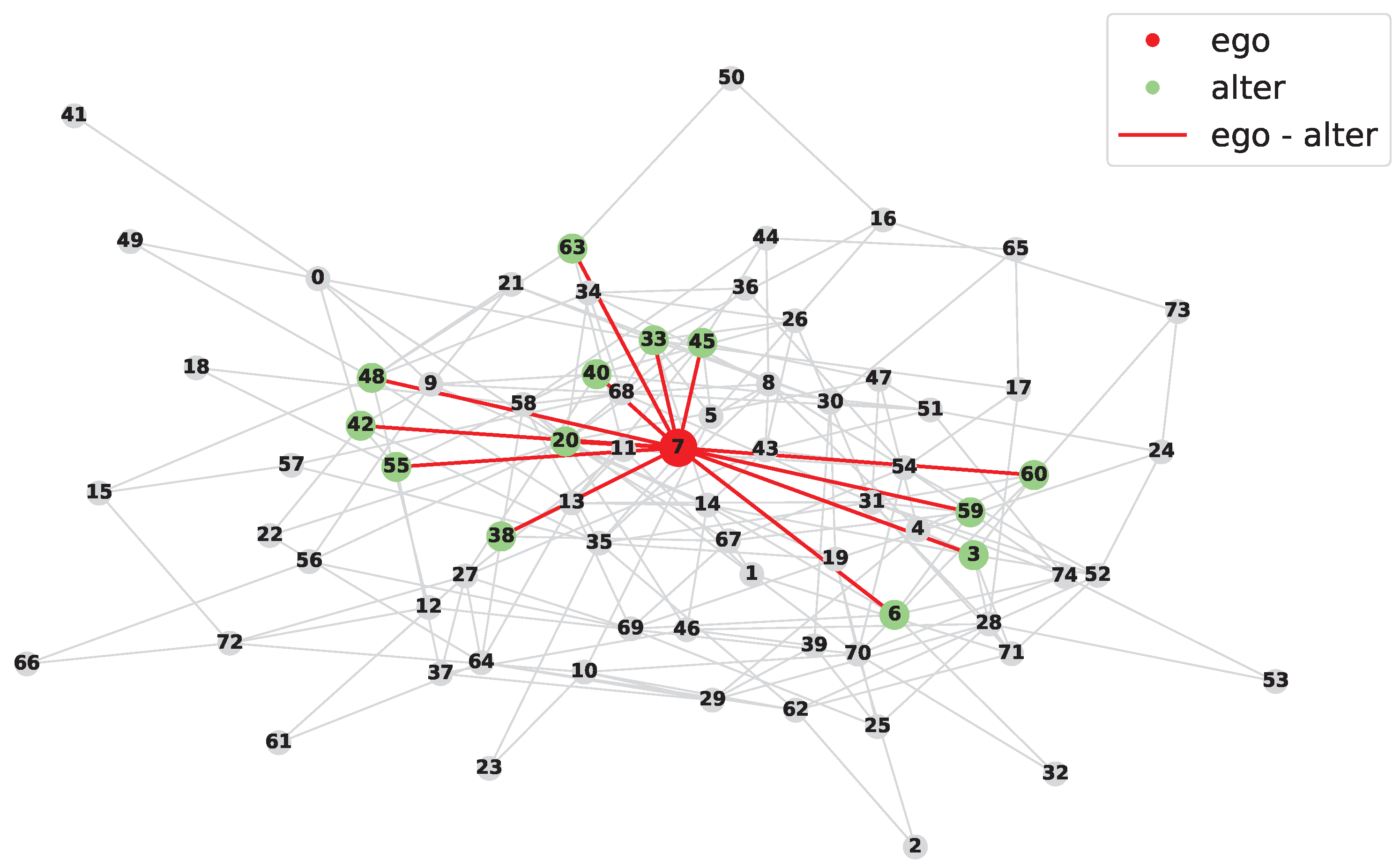
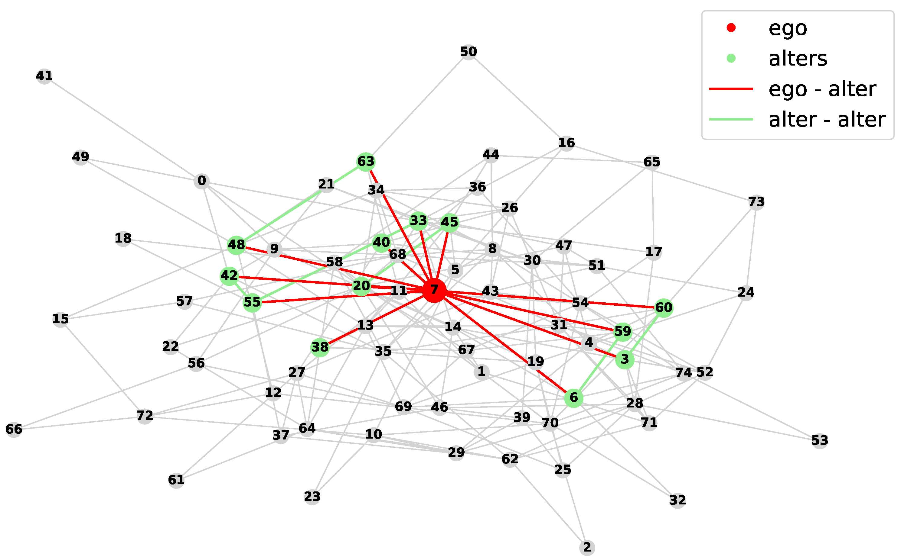
Figure 3, Figure 4 and Figure 5 show the construction of an ego network ${\mathcal{E}}_j$ from a node $u_j\in {\mathcal{U}}^{*}$. Recall that the users of ${\mathcal{U}}^{*}$ are a subset of the users of $\mathcal{U}$; therefore, each user of ${\mathcal{U}}^{*}$ corresponds to a node in $\mathcal{N}$. Consequently, the construction of the ego network of $u_j$ takes place on $\mathcal{N}$ starting from the node corresponding to $u_j$. Figure 3 shows a network $\mathcal{N}$ from which we start the construction of the ego network associated with Node 7, colored in red. Figure 4 shows the selection of the alter nodes, i.e., the nodes adjacent to Node 7 (colored in green). In this figure we also highlight the edges connecting the ego to the alters (colored in red). Figure 5 shows the complete ego network; this requires adding all the edges connecting two alters (colored in green).

Repeating this process for each node $u_j\in {\mathcal{U}}^{*}$ yields all the corresponding ego networks. Performing the union of the sets of nodes of all ego networks yields the set of nodes of ${\mathcal{N}}^{*}$, while performing the union of the sets of edges of all ego networks yields the set of edges of ${\mathcal{N}}^{*}$.

After constructing ${\mathcal{N}}^{*}$, our framework calculates and analyzes a set of statistics on the ego networks of ${\mathcal{N}}^{*}$. More specifically, it computes these statistics first considering all the ego networks of ${\mathcal{N}}^{*}$ altogether and then subdividing them based on the stance of the corresponding ego. As a result, there will be s groups, one for each stance of $\mathcal{S}$. The statistics analyzed by our framework are the following:

• Number of nodes;
• Number of edges;
• Density;
• Average sentiments of the comments posted;
• Average number of aggressive comments;
• Average number of non-aggressive comments;
• For each stance, average number of users following it;
• Average clustering coefficient.

By comparing the values of all these statistics and some of their ratios for both the ego networks of ${\mathcal{N}}^{*}$ and the ego networks associated with the influential users of each stance, our framework allows us to extract several insights about the polarization of influential users, as we will see in Section 4.4.

4. Results

In this section, we present the experiments we conducted to evaluate our framework. Specifically, in Section 4.1 we provide an overview of our experimental campaign. In Section 4.2, we describe the dataset used for our tests. In Section 4.3, we illustrate the experiments regarding community polarization. Finally, in Section 4.4 we present the experiments concerning the polarization of the most influential users.

4.1. Overview of Our Experimental Campaign

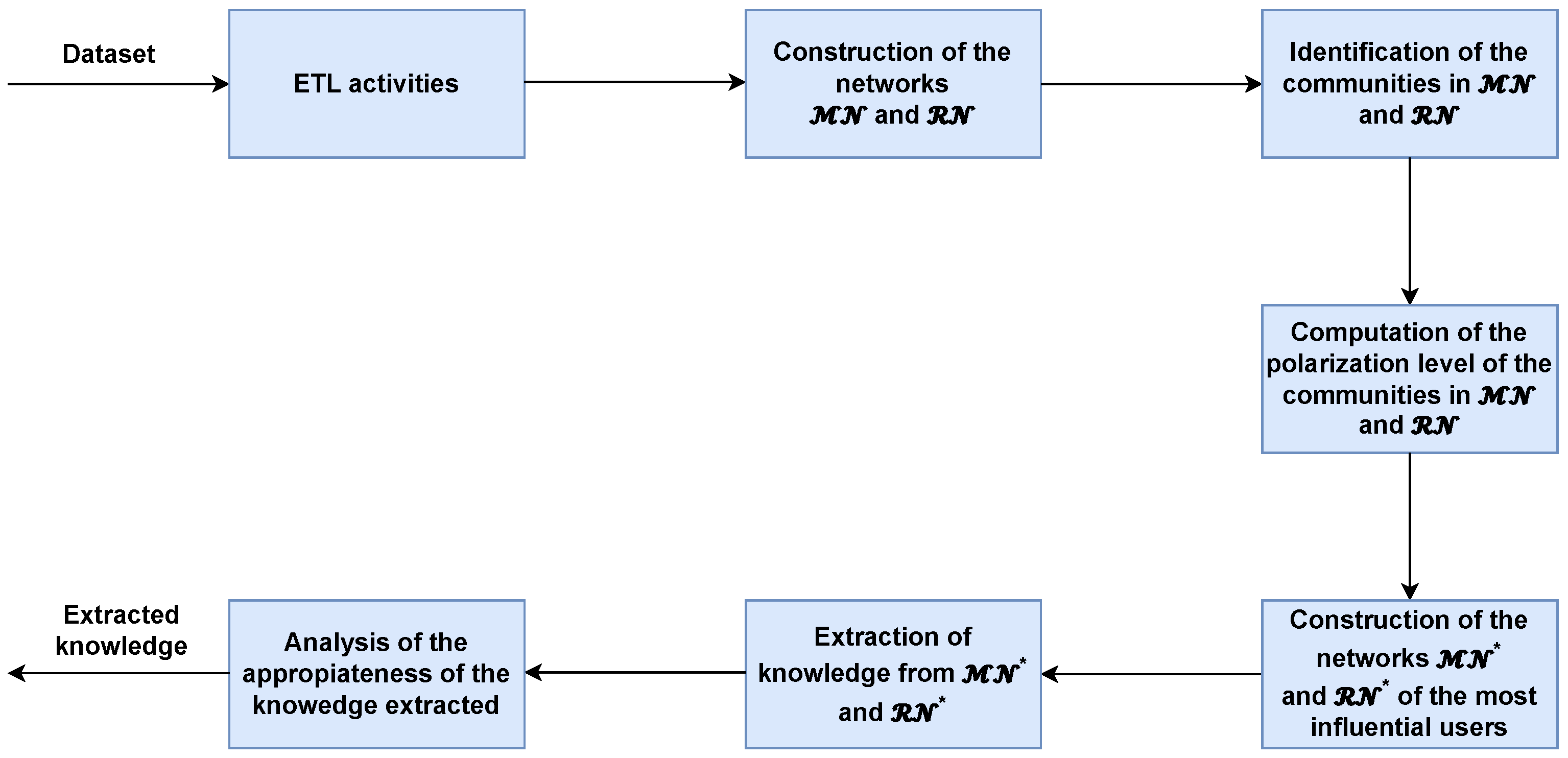
Our experimental campaign receives a dataset derived from X. The dataset stores comments on a certain topic that users of X have exchanged over time. Our campaign performs several tasks to verify (i) whether the communities derived from the dataset are polarized, and (ii) whether the most influential users in the dataset are polarized. To achieve these objectives, it follows the workflow shown in Figure 6.

As shown in the figure, we first perform Extraction, Transformation and Loading (ETL) activities on the source dataset. Then, we build two support networks, namely (i) $\mathcal{MN}$, which takes into account mentions, and (ii) $\mathcal{RN}$, which takes into account replies. Next, we identify the various communities in $\mathcal{MN}$ and $\mathcal{RN}$. For each community, we determine its polarization level, and consequently if it is polarized or not. At this point, we identify the most influential users in $\mathcal{MN}$ and $\mathcal{RN}$. Starting from the ego networks of these users, we then build two additional support networks ${\mathcal{MN}}^{*}$ and ${\mathcal{RN}}^{*}$. Then, we extract insights from these networks to determine the polarization level of the most influential users. Finally, we verify the appropriateness of the extracted information. The following sections first illustrate the workflow for each step described above, then provide a detailed description.

4.2. Dataset

In this section, we present our dataset, the Extraction, Transformation, and Loading (ETL) operations performed on it, as well as the results of some basic analyses and the corresponding validation.

4.2.1. Overview

We considered The Climate Change Twitter Dataset [33] as the starting dataset for our experimental campaign. It is derived from X and contains tweets about climate change published from 2006 to 2019.

Figure 7 shows the workflow we followed to prepare this dataset for our experimental campaign. As the figure shows, we initially filtered the data by year, selecting only 2018 and 2019. Afterward, we performed a hydration process to extract additional information concerning the tweets in the dataset. After reconstructing the metadata and content of all tweets, we computed several statistics on them, which allowed us to extract insights. Next, we removed neutral tweets, leaving only those that contributed to the polarization phenomenon. At this point, we shifted our focus from the tweets to the corresponding users. First, we calculated statistics on the users, removed neutral users, and identified those belonging to the two classes of believers and deniers. Next, we built the Mention Network $\mathcal{MN}$ to model all user mentions and the Reply Network $\mathcal{RN}$ to model all user replies. We then performed analyses on $\mathcal{MN}$ and $\mathcal{RN}$ to extract insights about the polarization of their users and communities. Finally, we validated these insights with human assistance. In the following, we illustrate each step of the workflow in detail.

4.2.2. Technical Details

Given the dataset, analyzing data over all reference time period (i.e., from 2006 to 2019) may introduce noise due to changes in context or user behavior that may occur during this time. To avoid this, we decided to narrow our scope and consider only the tweets published in the years 2018 and 2019, and thus only the discussions related to the last two years covered by our dataset. Each row in our dataset refers to a tweet and includes the attributes shown in

Table 1. Attributes of the dataset.

Attribute	Description
tweet_id	It is the unique identifier of the tweet.
created_at	It is the timestamp when the tweet was posted.
sentiment	It is the sentiment of the tweet. Its value varies in the real interval [−1,1]. A value less (resp., greater) than 0 indicates negative (resp., positive) sentiment.
stance	It is the stance of the tweet according to the climate change debate. If the tweet is in favor of the anthropogenic origin of climate change, it is labeled as believer. Conversely, if it is against that origin, it is labeled as a denier. Finally, if it maintains a neutral position on this issue, it is labeled as neutral.
aggressiveness	It is the tone and demeanor of the tweet. If the inherent language is confrontational, the tweet is classified as aggressive; otherwise, it is classified as non-aggressive.
topic	It is the topic discussed in the tweet.

.

The stance attribute is particularly important for our analysis and represents the result of the function $\sigma \left(c_i\right)$ (see Section 3.2) when a tweet $c_i$ is given as input. It serves as a classification label for tweets; in fact, it allows us to classify them based on their stance with respect to the hypothesis that climate change is human-induced. Tweets that agree with this hypothesis are labeled as “believers”, those that disagree with it are classified as “deniers”, and those that do not take a position on this hypothesis are labeled as “neutrals”. The authors of the Climate Change Twitter dataset inferred the stance of the tweets using transfer learning. To do this, they trained a BERT-based classifier on another publicly available dataset of tweets about climate change, which was already labeled, and used the classifier thus trained to label each tweet in their dataset [33].

Due to storage issues, the Climate Change Twitter dataset does not contain all of the useful information for our analysis. To obtain all the tweet details, a hydration process was necessary. Such a process converted tweet identifiers into full tweets, extracting all associated metadata such as text content, user information (including username and user ID), timestamps (indicating when the tweet was created), and engagement metrics (such as the number of likes and retweets). This process began with the collection of tweet identifiers and then interacted with the X API. Access to the API required authentication, which involved creating a developer account and obtaining the necessary credentials. Strategies were implemented to effectively handle the rate limitations imposed by the API (e.g., delays between successive requests). After successfully hydrating the tweet IDs, the enriched data was stored for further analysis. To perform tweet hydration efficiently, we used Hydrator (https://github.com/docnow/hydrator, accessed on 2 January 2023). We carried out the hydration task in January 2023 before X denied access to its data. By using the unique identifier of a tweet, Hydrator allowed us to obtain additional key information about it. Specifically, we first extracted the author of the tweet. Then, we determined whether it was posted as a result of a reply or a mention interaction and identified the referenced author. Recall that on X, a reply is an interaction in which a user responds directly to another user’s tweet. Instead, a mention occurs when a user refers to another within a tweet. In

Table 2. Attributes of the dataset.

Attribute	Description
tweet_id	It is the unique identifier of the tweet.
user_id	It is the unique identifier of the author of the tweet.
in_reply_to_user_id	If the tweet is a reply to another tweet, it is the identifier of the recipient of the reply.
user_mentions_id	If the tweet mentions another user, it is the identifier of the user mentioned.

, we illustrate the attributes obtained after the hydration process. The interested reader can find the complete dataset adopted in our experiments at the GitHub address: https://github.com/Michele997/Climate-Change-Debate-Polarization, accessed on 1 August 2025.

Once the hydration process terminated, we had a dataset with a set of attributes useful for performing a variety of analyses. The first analysis concerned the number of users and tweets following each stance. The results obtained are shown in

Table 3. Some statistics of the hydrated dataset.

Statistic	Value
Number of users	1,435,545
Number of tweets	4,190,961
Number of mentions	3,130,909
Number of replies	454,073
Minimum number of tweets per user	1
Average number of tweets per user	2.92
Maximum number of tweets per user	31,762
Number of believer tweets	3,314,625
Number of denier tweets	254,528
Number of neutral tweets	622,198

.

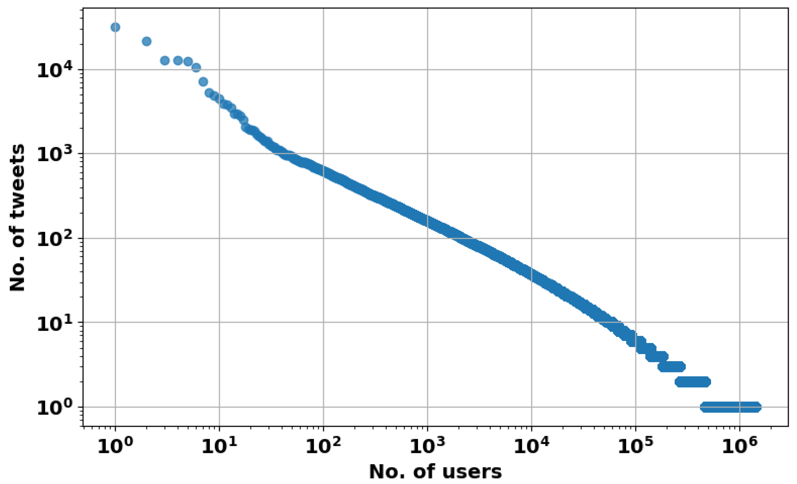
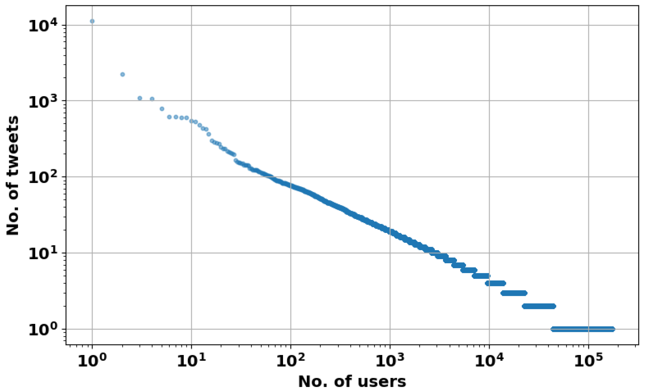
From the analysis of this table, we can see that the average number of tweets per user is low while the maximum number of tweets posted by a user is high. This is not surprising since, as it is generally the case in OSNs, it is possible to hypothesize that the distribution of the number of tweets against the number of users (shown in Figure 8) follows a power law. To verify the correctness of this hypothesis, we fit the distribution of the number of tweets per user to a power law model and calculated the corresponding values of the parameters a and D. a represents the scaling exponent and defines how fast the probability of large values decreases. It must be greater than 1; its typical values in networks are between 2 and 3 [64]; the higher its values, the steeper the power law. D represents the Kolmogorov–Smirnov distance [65] between the empirical data and the fitted power law model; the smaller its value, the better the fit. In our case, $a=2.6497$ and $D=0.0065$; this indicates that the distribution of the number of tweets per user does indeed follow a power law, and that the slope of this power law is quite steep. A large portion of tweets (i.e., 79.09%) follow the believer stance. Then, there are tweets following the neutral stance (14.84%) and, finally, tweets following the denier stance (6.07%).

Observe that the percentage of neutral tweets is very low compared to that of believer tweets and denier tweets, which as a whole represent polarized tweets. In particular, we have that neutral tweets represent 14.84% of the tweets, while polarized tweets are equal to 85.16% of total tweets. This result is extremely important because it allows us to remove neutral tweets from our dataset and focus only on polarized tweets. Therefore, we can focus on the topic of interest in our research, i.e., polarization, removing the confounding elements without causing significant bias in the data. In fact, if the percentage of neutral tweets had been substantial (i.e., comparable, or even greater than that of polarized tweets), removing neutral tweets would have led to a strong bias in the data, as we would have excluded the most representative stance (or, in any case, a very representative stance) from the dataset, which could have also led to a strong bias in the results. In our case, however, this risk does not exist. Furthermore, moving from the examination of tweets to that of users, which are the entities we are most interested in, we can observe that the average number of tweets per user makes it plausible that the proportions of neutral and polarized elements existing for tweets cannot be biased for users. Consequently, the proportion of users following the neutral stance is likely to be very small (this will be verified below). Therefore, we can remove these users from the dataset without running the risk of removing an important stance, or even the dominant stance, of users. As a consequence of all these considerations, we can remove both neutral tweets and neutral users from the dataset and study only the two extreme positions (i.e., believers and deniers), which is the ideal scenario for investigating the polarization phenomenon.

After removing the neutral tweets, we obtained a new dataset whose characteristics are shown in

Table 4. Some statistics of the dataset after the removal of neutral tweets.

Statistic	Value
Number of users	1,329,329
Number of tweets	3,569,153
Number of mentions	2,666,379
Number of replies	386,702
Minimum number of tweets per user	1
Average number of tweets per user	2.86
Maximum number of tweets per user	31,762
Number of believer tweets	3,314,625
Number of denier tweets	254,528

.

From the analysis of this table, we can see that the number of users decreased by 7.40%, which is the percentage of users who published only neutral tweets. As we hypothesized, this percentage is very low compared to the percentage of polarized users (92.60%), and the removal of neutral users does not cause a significant bias in the investigation of the polarization phenomenon. We also observe that the dataset is unbalanced, since 92.87% of the tweets follow the believer stance, while 7.13% of them follow the denier stance.

Since the ultimate entities of interest are users and not tweets, we continued our analysis by classifying also users in believers and deniers. Specifically, we classified a user as a believer (resp., denier) if she posted more believer (resp., denier) tweets than denier (resp., believer) ones. If a user posted the same number of believer tweets and denier tweets, we classified her as neutral and removed her from the dataset. At the end of this task, we removed 22 further users and their tweets from the dataset (specifically, 64 denier tweets and 64 believer tweets). After these operations, we obtained our reference dataset for the experimental campaign, whose basic statistics are shown in

Table 5. Some statistics of the final dataset.

Statistic	Value
Number of users	1,329,307
Number of tweets	3,569,089
Number of mentions	2,666,332
Number of replies	386,696
Minimum number of tweets per user	1
Average number of tweets per user	2.86
Maximum number of tweets per user	31,762
Number of believer tweets	3,314,561
Percentage of believer tweets	92.87%
Number of denier tweets	254,464
Percentage of denier tweets	7.13%
Number of believer users	1,233,779
Percentage of believer users	92.81%
Number of denier users	95,528
Percentage of denier users	7.19%

.

Before proceeding, it is important to clarify how the characteristics of our dataset align with the objectives of this paper. Our goal is essentially to define a framework for analyzing polarization in OSNs. In order to evaluate the framework’s performance, we need a dataset in which the comments and their corresponding authors are polarized. From this perspective, our dataset is well suited since, after the aforementioned refinement activities, tweets and users are polarized. However, a potential problem with this dataset is that it is heavily skewed toward one stance (in fact, 92.81% of users are believers). Similar imbalances are common in polarization literature [66,67,68], since finding a highly polarized and perfectly balanced dataset is extremely difficult. Data analysis provides upsampling and downsampling techniques to balance classes artificially [59]. However, applying these techniques to our dataset would distort its structure. In fact, in our case tweets are linked to users and often correspond to mentions or replies. Upsampling the minority class (deniers) would require generating fictitious users to maintain the tweet-user distribution, which would undermine analyses focused on real user behavior. Conversely, downsampling the majority class (believers) would entail removing approximately 90% of the tweets and users, yielding a considerably smaller, more fragmented network whose properties differ markedly from those of the original network. Therefore, we cannot use upsampling or downsampling techniques in our case.

To ensure that our results are valid and do not depend on class imbalance, we performed significance tests involving null models. These models preserved the characteristics of the original networks, such as the degree of their nodes, as well as the level of imbalance between believers and deniers in terms of both tweets and users. Using significance tests and null models that preserve the particular characteristics of the original networks ensures that the validity of our framework does not depend on a specific configuration of the ratio between user stances and/or tweet stances. In fact, our framework can be applied to any dataset, regardless of its level of imbalance, provided that this level is reproduced in the null models of the corresponding significance tests.

At this point, however, in order to carry out our analyses on polarization, we need a metric that easily indicate the initial polarization level, as well as its increase or decrease due to the experiment we are conducting. In other words, it is necessary that any change, even small, in the initial polarization level, due to some aspect that we study in the tests, is clearly reflected in this measure. The most reasonable measure with such characteristics that we identified was the polarization ratio:

$$r_{bd}={\displaystyle \frac{Numberofbelieverusers}{Numberofdenierusers}}$$

(12)

In our reference dataset the value of $r_{bd}$ is 12.91. In the following experiments, we will see how the value of $r_{bd}$ varies after each test. A decrease (resp., increase) in it will imply less (resp., more) polarization.

After introducing $r_{bd}$, a final consideration about the imbalance of our dataset is in order. As mentioned above, all our analyses will take into account the differences in the value of $r_{bd}$ before and after each experiment. Studying the differences between the values of $r_{bd}$ rather than the absolute values of $r_{bd}$ allows us to conduct analyses that eliminate, or at least significantly reduce, the class imbalance problem that characterizes the initial dataset.

In addition, in each experiment involving the polarization ratio that we performed, we compared the results returned with those for a null model obtained using the QAP test [69]. The latter is a permutation test suitable for testing hypotheses about quantities that depend on the labels of the nodes of a network $\mathcal{N}$ in which its structure remains fixed [69]. In particular, given a parameter $pa$ derived from $\mathcal{N}$, we want to know whether its values are statistically different from what we would expect from chance alone. The QAP test works by permuting node labels while preserving the underlying network structure, thus obtaining a reference null model ${\mathcal{N}}^{\prime }$. In our application of the QAP test, we permuted the node labels $z=10,000$ times and calculated the value of $pa$ on this set of null models. Finally, we calculated the statistical significance of $pa$ as follows: let $g_{pa}$ be the value of $pa$ in $\mathcal{N}$ and let $g_1,g_2,\dots ,g_z$ be the values of $pa$ in the z null models. We calculated the p-value as:

$$p_{pa}={\displaystyle \frac{{\sum }_{i=1}^z\lambda (g_i>g_{pa})}{z}}$$

(13)

where $\lambda :\mathcal{B}\to \{0,1\}$ is the indicator function that returns 1 if the condition in parenthesis is true, 0 otherwise. Once we have computed $p_{pa}$, we considered $pa$ statistically significant if and only if $p_{pa}<0.05$. The use of the QAP test assures us that the results obtained are due to the presence of real polarization phenomena in the network and not to chance.

As previously pointed out, we built two separate networks for our experiments. The first, denoted as $\mathcal{MN}$, represents only users who interacted through mentions, while the second, denoted as $\mathcal{RN}$, considers only users who replied to tweets. Specifically, in $\mathcal{MN}$ (resp., $\mathcal{RN}$) nodes represent users who posted at least one mention (resp., reply) tweet. An edge exists between two nodes if at least one of the two users interacted with the other via a mention (resp., reply) tweet. The main characteristics of the networks $\mathcal{MN}$ and $\mathcal{RN}$ are shown in

Table 6. Some statistics of $\mathcal{MN}$ and $\mathcal{RN}$.

Statistic	$\mathcal{MN}$	$\mathcal{RN}$
Number of nodes	1,255,244	293,226
Number of edges	2,266,566	308,471
Density	2.88 $·{10}^{-6}$	7.18 $·{10}^{-6}$
Minimum degree of a node	1	1
Average degree of a node	3.61	2.10
Maximum degree of a node	41,012	9434

. From the analysis of this table, we can observe that the mention relationship is much more used than the reply relationship to interact with other users. We calculated the distributions of the number of tweets against the number of users for $\mathcal{MN}$ and $\mathcal{RN}$. They are reported in Figure 9.

As can be seen in the figure, both these distributions follow a power law. In particular, for the distribution on top we have that $a=2.8018$ and $D=0.0049$, while for the distribution on bottom we have that $a=2.5581$ and $D=0.0114$. The very low values of D confirm that the two distributions fit the power law model very well, while the high values of a indicate that the two power law distributions are characterized by a very steep decay.

4.2.3. Evaluation of the Labels of the Original Dataset

In the previous section, we have seen that the tweets in our dataset are labeled as believer tweets (3,314,561) and denier tweets (254,464). We have also seen that this labeling was already provided with the dataset [33]. Since our next analyses refer to it, so that if it is invalid the results are biased, we decided to carry out its validation with human assistance. To perform such a task, we took the following steps:

• We constructed 10 sets of tweets; each set contained 250 believer tweets and 250 denier tweets randomly selected from the reference dataset.
• We asked 10 different human experts to label the constructed sets of tweets; specifically, we assigned one set to each expert and, of course, for the tweets in the set, we did not report their stance specified in the dataset so that the expert would not be influenced by this information.
• We constructed the confusion matrix between the stances given by the experts and the ones in the dataset. This matrix is reported in Figure 10.
• We calculated the values of some quality metrics, namely:

  –

  Precision = ${\displaystyle \frac{TP}{TP+FP}}={\displaystyle \frac{2472}{2472+34}}=0.9864$

  –

  Recall (Sensitivity) = ${\displaystyle \frac{TP}{TP+FN}}={\displaystyle \frac{2472}{2472+28}}=0.9888$

  –

  Specificity = ${\displaystyle \frac{TN}{TN+FP}}={\displaystyle \frac{2466}{2466+34}}=0.9864$

  –

  Accuracy = ${\displaystyle \frac{TP+TN}{TP+FN+FP+TN}}={\displaystyle \frac{2472+2466}{2472+28+34+2466}}=0.9876$

Examining the results obtained, we can see that all the quality metrics have very high values; in fact, all of these values are higher than 0.98. As a consequence, we can conclude that the labeling of the tweets present in the source dataset is reliable and therefore the results we obtain in the next sections are not due to a dataset bias.

4.3. Analysis of Community Polarization

In this section, we present our analysis of community polarization within the networks $\mathcal{MN}$ and $\mathcal{RN}$.

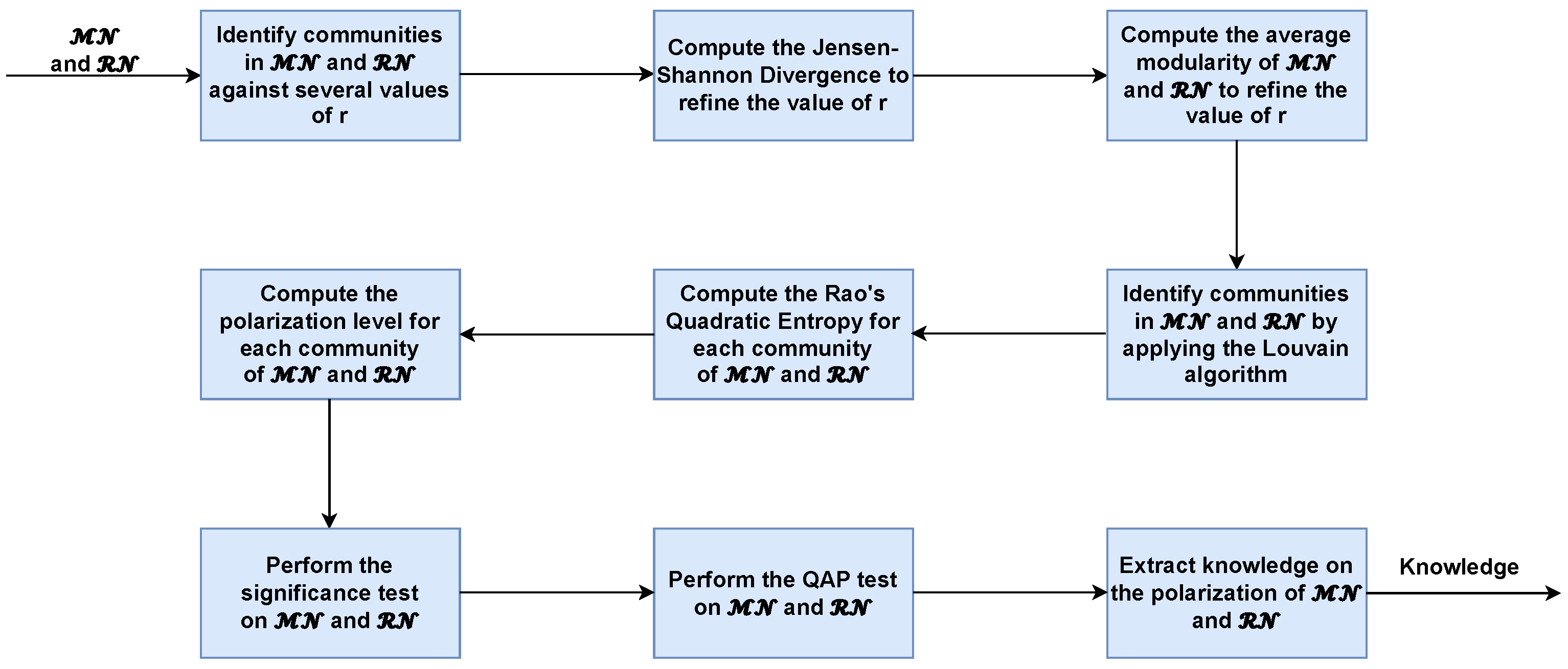
Figure 11 illustrates the workflow we followed to determine the polarization level of user communities in $\mathcal{MN}$ and $\mathcal{RN}$. As shown in the figure, the first step was to determine the optimal value of the parameter r of the Louvain algorithm (see Section 3.3.1) by analyzing the communities of $\mathcal{MN}$ and $\mathcal{RN}$ obtained from the variation of the values of this parameter. Next, we further refined the value of r by calculating the Jensen–Shannon Divergence and the average modularity of $\mathcal{MN}$ and $\mathcal{RN}$. After these steps, we obtained the final value of r. Then, by applying the Louvain algorithm with the value of r thus determined, we identified the communities of interest in $\mathcal{MN}$ and $\mathcal{RN}$. Next, we calculated the Rao’s Quadratic Entropy for each community in $\mathcal{MN}$ and $\mathcal{RN}$. To determine if these results were related to reality or chance, we performed a significance test on $\mathcal{MN}$ and $\mathcal{RN}$, followed by a QAP test on the same networks. After these tests, we determined that the polarization of the communities was real and not due to chance. Finally, we performed further analyses on the polarized communities of $\mathcal{MN}$ and $\mathcal{RN}$ to detect insights about them. In the following, we illustrate each step of the workflow in detail.

4.3.1. Identification of Communities

The first step of our workflow involved the identification of communities within $\mathcal{MN}$ and $\mathcal{RN}$ through the application of the Louvain algorithm. In our experiments, we used a multi-threaded parallel implementation of this algorithm operating on compressed sparse matrices. This version parallelizes the local-moving phase (i.e., at each iteration, each node is reassigned to the neighboring community that maximizes the modularity gain) and processes the connected components independently. This choice allowed us a very quick detection of communities in our graph that consists of 1.25 million nodes. In particular, using a server equipped with an Intel(R) Xeon(R) W5-3435X CPU at 3.10 GHz, 128 GB of RAM, and an NVIDIA RTX A2000 GPU with 12 GB of memory, running a single instance of the Louvain algorithm on the network $\mathcal{MN}$ took an average of 104.36 s, while running it on the network $\mathcal{RN}$ took an average of 13.93 s. Even when a given experiment requires executing the Louvain algorithm multiple times on the same network, the total time increases proportionally to the number of executions, but remains in the same order of magnitude. These timings allow us to use the Louvain algorithm in our framework, even in those cases that require extensive experimental campaigns involving the repetition of a test numerous times as the values of one or more parameters vary. Furthermore, it is important to note that the study of community polarization is inherently offline, given its objectives and applications. Typically, such a study involves defining a business case, designing one or more analyses, and finally performing them. In such a scenario, running the Louvain algorithm with the above-provided timing and the possibility of parallelizing executions takes time that can easily be absorbed by the normal flow of activities.

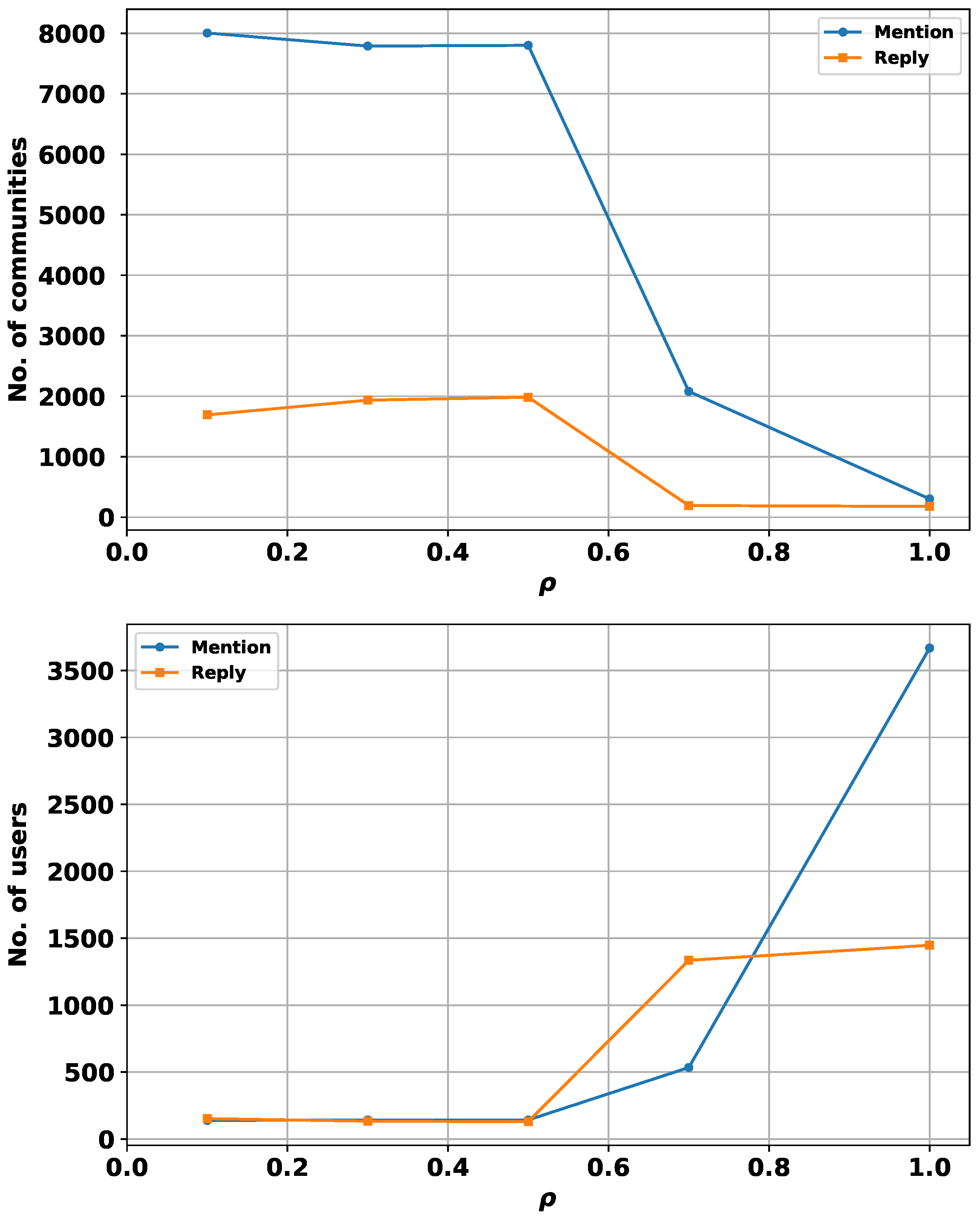
To determine the most appropriate value for the hyperparameter r of the Louvain algorithm, we conducted a systematic tuning process and evaluated several candidate values. In particular, we considered the following set of values for r: $\{0.1,0.3,0.5,0.7,1.0\}$. We ran the Louvain algorithm on both $\mathcal{MN}$ and $\mathcal{RN}$ for each value of r, analyzing the structure of the communities returned. We based our evaluation on two complementary indicators, namely: (i) the total number of communities identified, and (ii) the average number of users per community. These two metrics allow us to understand the partition’s granularity and cohesion, respectively. The results are illustrated in Figure 12. In particular, the top of this figure shows that as r increases the number of communities identified decreases progressively. In parallel, the bottom of the same figure shows that the average number of users per community increases as r increases, indicating an increasingly aggregated community structure. This trend is consistent with the known behavior of the Louvain algorithm. A particularly relevant aspect emerges when we observe the transition from $r=0.5$ to $r=0.7$. In both graphs, this transition is characterized by a clear change in the two curves. Indeed, the number of communities decreases substantially, while their average size increases significantly. This behavior suggests a shift from a fine, well-structured division of users to an overly coarse division, in which oversized communities allow users with weak or indirect connections to coexist. These aggregations compromise the readability and analytical value of the community structure, particularly in studies on polarization, where identifying cohesive and ideologically homogeneous groups is essential. For this reason, we limited our analysis to values of r less than or equal to 1. For values greater than 1, the network often collapses into a few large macro-communities that are too big to be useful for polarization analysis. Preliminary tests conducted with $r>1$ (not reported here due to space limitations) confirmed this trend, which ultimately leads to very uninformative results. Furthermore, high values of r (and our preliminary tests have shown that $r=1$ is already a high value for this experimental scenario) can compromise the principle of modularity optimization on which the Louvain algorithm is based, returning partitions that no longer reflect the natural structure of real networks.

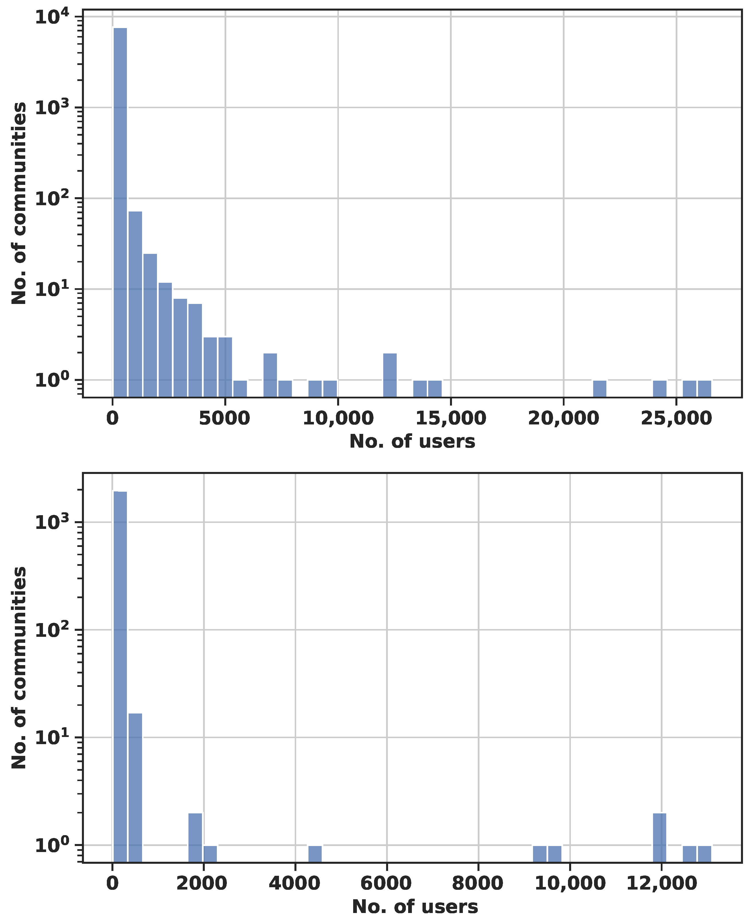
To give an idea of the reference scenario, in Figure 13 we show the distribution of communities in $\mathcal{MN}$ and $\mathcal{RN}$ with $r=0.5$. From the analysis of this figure, we can see that $\mathcal{MN}$ has a greater number of communities than $\mathcal{RN}$. In addition, $\mathcal{MN}$ has a higher average number of users per community than $\mathcal{RN}$; specifically, the latter is 142.47 in $\mathcal{MN}$ while it is 129.87 in $\mathcal{RN}$. This result can be explained by considering that $\mathcal{MN}$ has a greater number of nodes and edges than $\mathcal{RN}$.

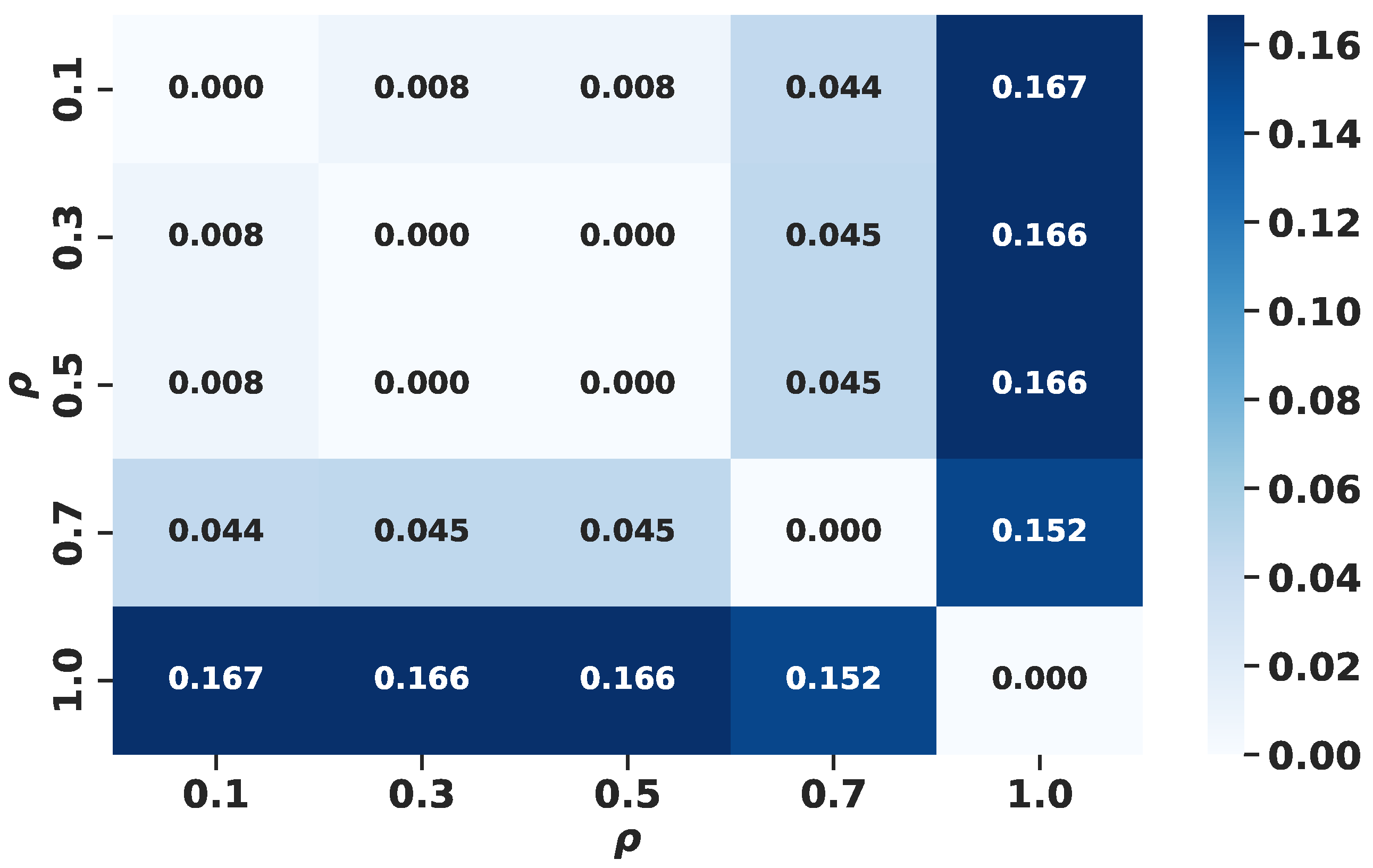
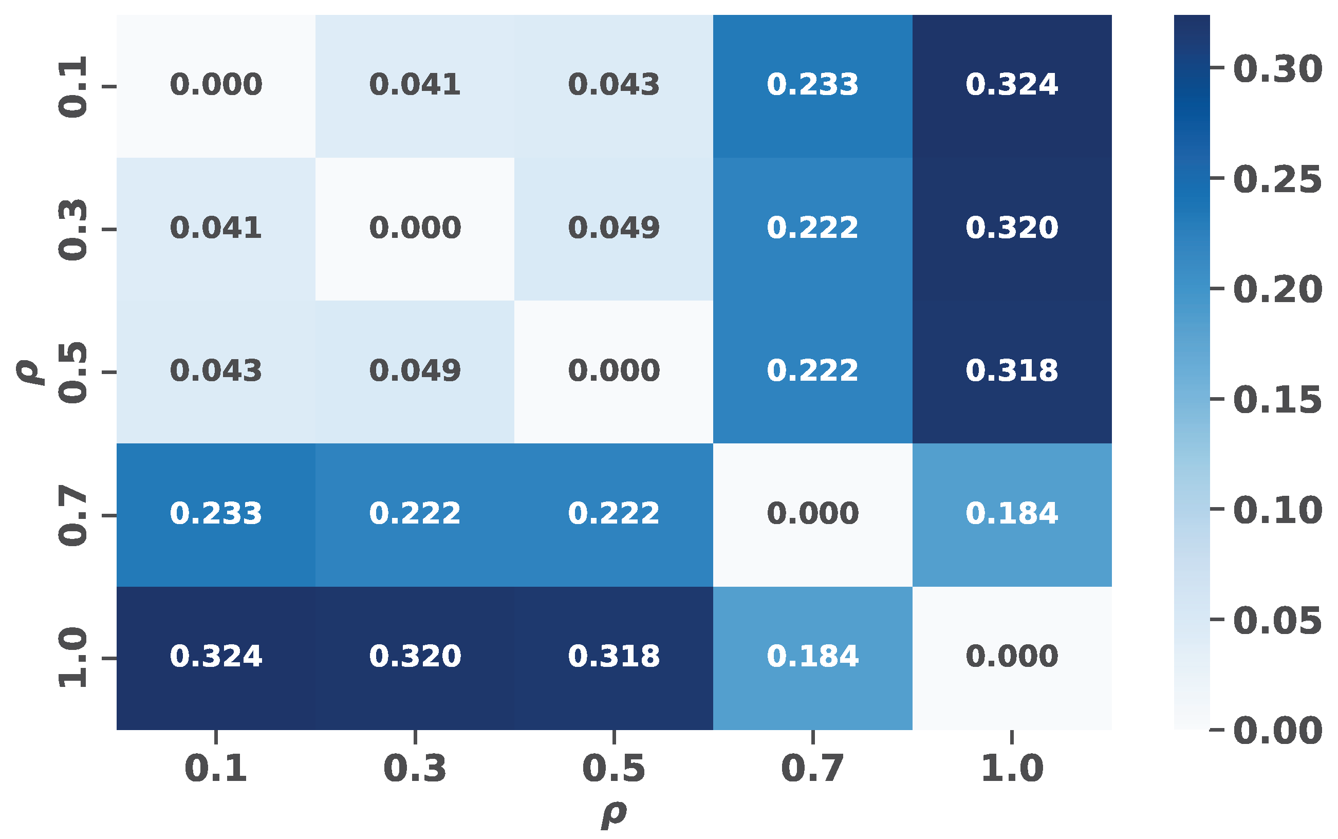
As an additional tuning task, we constructed the distribution of users in the communities for different values of r and then computed the Jensen–Shannon Divergence (JSD) [70] between each pair of distributions. JSD quantifies the similarity between two probability distributions. Its values are in the real range $[0,1]$; the lower the values, the more similar the distributions. Importantly, unlike other divergence measures, JSD is always finite and symmetric, making it particularly suitable for comparing discrete distributions, such as those involving users in communities. Since JSD works on probability distributions, we first normalized each of our distributions so that the sum of their entries is equal to 1. Then, for each pair of values of r, we computed the value of JSD between the corresponding normalized distributions for both the networks $\mathcal{MN}$ and $\mathcal{RN}$. The resulting heatmaps are shown in Figure 14.

Looking at the top of the figure, we can see that, in the case of $\mathcal{MN}$, the distributions for $r=0.1$, $r=0.3$ and $r=0.5$ are very similar to each other. The distribution for $r=0.7$ shows some dissimilarity with the three previous ones and also with the distribution for $r=1.0$. The latter has an even greater dissimilarity with the first three distributions. When we move from $\mathcal{MN}$ to $\mathcal{RN}$ (bottom of the figure), the trends seen for $\mathcal{MN}$ are not only confirmed, but strengthened. The distributions for $r=0.1$, $r=0.3$ and $r=0.5$ are very similar to each other and differ from the one for $r=0.7$ and even more from the distribution for $r=1.0$. As a result, we can observe that in both $\mathcal{MN}$ and $\mathcal{RN}$ there is a clear separation between two regions, namely a region of stability that occurs for $r\in \{0.1,0.3,0.5\}$ and a range of structural changes that occurs for $r\in \{0.7,1.0\}$. This separation, and more generally the results of this tuning task, are completely consistent with those of the first search task described above.

Therefore, at the end of the two tuning tasks, it seems reasonable to restrict the possible values of r to the set $\{0.1,0.3,0.5\}$.

To choose the final value of r, we considered the average modularity of the communities in $\mathcal{MN}$ and $\mathcal{RN}$ obtained by the Louvain algorithm. Recall that modularity is an index of cohesion [58]. Its value is in the real range $[0,1]$; the higher its value, the more cohesive the corresponding communities. Consequently, it makes sense to calculate the value of modularity in $\mathcal{MN}$ and $\mathcal{RN}$ for the three possible values of r and to choose the value guaranteeing the highest modularity. In

Table 7. Average modularity values for the communities of $\mathcal{MN}$ and $\mathcal{RN}$ against the values of r.

	$\mathcal{MN}$	$\mathcal{RN}$
$r=0.1$	0.5085	0.6800
$r=0.3$	0.5188	0.8076
$r=0.5$	0.5836	0.8423

, we report the average modularity values for the communities of $\mathcal{MN}$ and $\mathcal{RN}$ obtained for the three values of r. As can be seen from this table, for both networks the maximum modularity values are obtained at $r=0.5$. Therefore, we decided to take this value of r whenever we used the Louvain algorithm in our tests.

4.3.2. Analysis of Polarization Within Communities

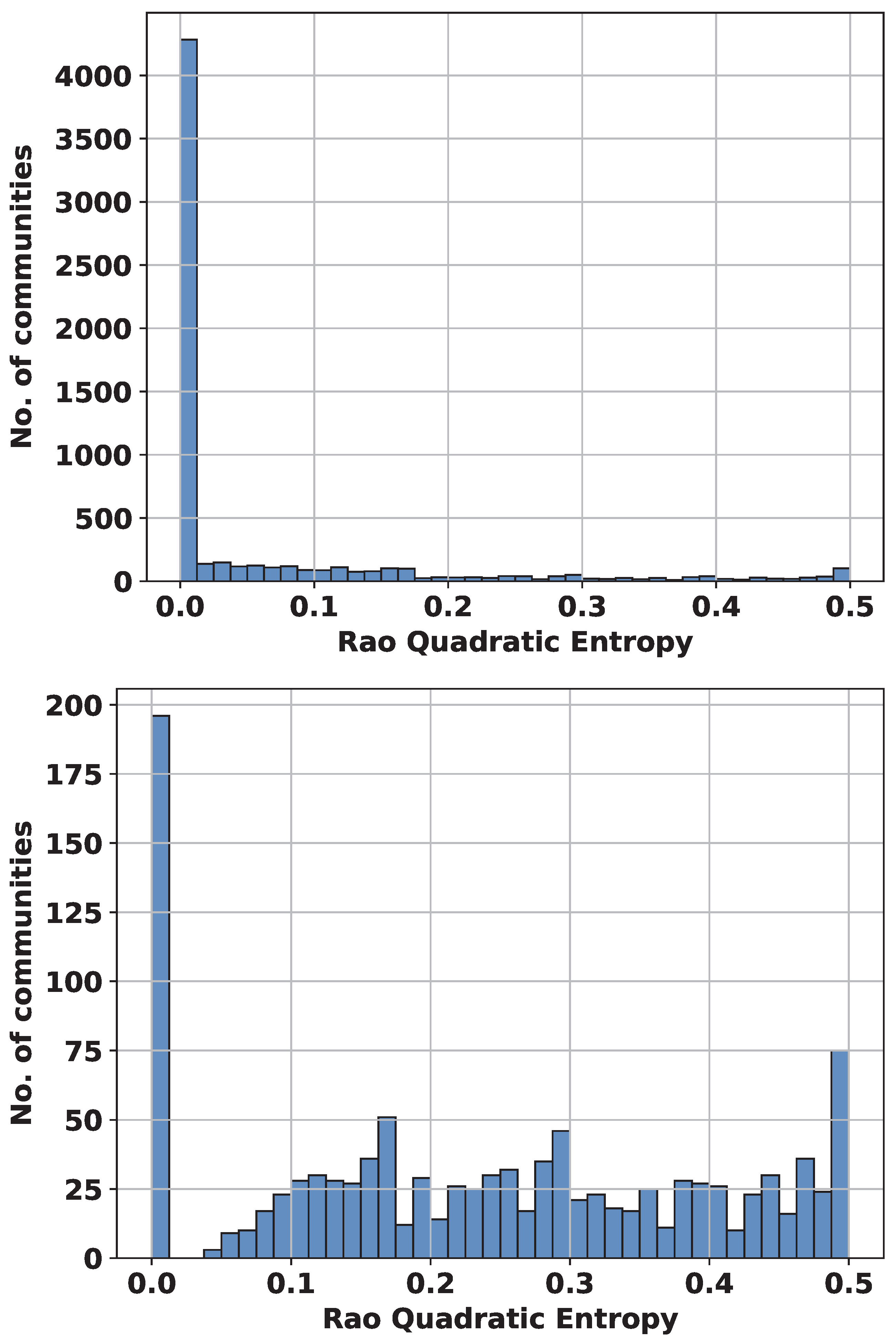
To analyze polarization within communities, we adopted the Rao’s Quadratic Entropy $RI$ (see Equation (3)). Specifically, we employed this index to determine the distribution of believers and deniers within communities. In Section 3.3.1, we have seen that: (i) given a community $q_l\in Q$, the lower the value of $R{I}_l$, the higher its polarization; (ii) if there are two stances to consider for investigating polarization, the Rao’s Quadratic Entropy can reach a maximum value of 0.5. Figure 15 shows the distribution of $RI$ for the communities in $\mathcal{MN}$ and $\mathcal{RN}$. From the analysis of this figure we can see that most of the communities are polarized. This phenomenon is particularly pronounced for the network $\mathcal{MN}$ where the vast majority of communities (i.e., more than 4000) have a value of $RI$ of 0. This trend is also observed for the network $\mathcal{RN}$ albeit it is less pronounced.

However, it is essential to validate these results before drawing conclusions. The need for validation stems from the fact that the initial data for the analysis had a significant imbalance of user stances. For validation, we adopted the significance test described in Section 3.3.1 and the QAP test described in Section 4.2.

As for the significance test, we employed the null model as a benchmark to determine whether there are significant deviations from what we might expect from a random chance. To do this, we constructed a null model ${\mathcal{MN}}^0$ from $\mathcal{MN}$ and a null model ${\mathcal{RN}}^0$ from $\mathcal{RN}$. After that, we applied the Louvain algorithm to ${\mathcal{MN}}^0$ and ${\mathcal{RN}}^0$ to obtain communities, and then calculated the distribution of $RI$ on them. The results obtained are shown in Figure 16.

In

Table 8. Average number of communities and their size for $\mathcal{MN}$ and $\mathcal{RN}$ and their null models.

Statistic	$\mathcal{MN}$	${\mathcal{MN}}^0$	$\mathcal{RN}$	${\mathcal{RN}}^0$
Number of communities	7801	7585	1984	3214
Average size of communities	142.47	93.12	129.87	41.84

, we report the number of communities with more than 10 members found in $\mathcal{MN}$ and $\mathcal{RN}$ and their corresponding null models. This table also shows the average size of these communities. From its analysis we can see that, as far as $\mathcal{MN}$ and ${\mathcal{MN}}^0$ are concerned, there are no significant differences in the community number, while community size is greater in $\mathcal{MN}$ than in ${\mathcal{MN}}^0$. In contrast, important differences can be observed for $\mathcal{RN}$ and ${\mathcal{RN}}^0$. In fact, we can note that the number of communities in ${\mathcal{RN}}^0$ is much greater than that in $\mathcal{RN}$, while their average size is less than a third.

In

Table 9. Mean and variance of the distributions of the percentages of user stances within $\mathcal{MN}$ and $\mathcal{RN}$.

User Stance	Mean $\mathcal{MN}$	Variance $\mathcal{MN}$	Mean $\mathcal{RN}$	Variance $\mathcal{RN}$
Believers	94.06%	0.078	62.95%	0.044
Deniers	5.94%	0.014	13.60%	0.014

(resp.,

Table 10. Mean and variance of the distributions of the percentages of user stances within ${\mathcal{MN}}^0$ and ${\mathcal{RN}}^0$.

User Stance	Mean ${\mathcal{MN}}^0$	Variance ${\mathcal{MN}}^0$	Mean ${\mathcal{RN}}^0$	Variance ${\mathcal{RN}}^0$
Believers	84.09%	0.011	93.88%	0.012
Deniers	15.91%	0.003	6.12%	0.005

), we show the mean and variance of the distributions of the percentages of user stances within the communities of the networks $\mathcal{MN}$ and $\mathcal{RN}$ (resp., ${\mathcal{MN}}^0$ and ${\mathcal{RN}}^0$).

Looking at the mean percentages in $\mathcal{MN}$ and ${\mathcal{MN}}^0$ we can observe that in ${\mathcal{MN}}^0$ the value of the mean percentage of deniers is much higher than in $\mathcal{MN}$ (more than twice as high). The opposite effect is observed in $\mathcal{RN}$ and ${\mathcal{RN}}^0$. In fact, in $\mathcal{RN}$ the value of the mean percentage of deniers is more than twice as high as in ${\mathcal{RN}}^0$. The differences between $\mathcal{MN}$ and $\mathcal{RN}$ and the corresponding null models become even more pronounced on the variances; in fact, the latter are much greater in $\mathcal{MN}$ and $\mathcal{RN}$ than in ${\mathcal{MN}}^0$ and ${\mathcal{RN}}^0$ for both believers and deniers.

Table 9 and Table 10, along with Figure 16, allow us to hypothesize that there are significant differences between $\mathcal{MN}$ and ${\mathcal{MN}}^0$ and between $\mathcal{RN}$ and ${\mathcal{RN}}^0$ and that these differences are not due to chance. To test this hypothesis, we decided to apply the Kolmogorov–Smirnov test to the distributions of $RI$ in the communities of $\mathcal{MN}$ and ${\mathcal{MN}}^0$ (resp., $\mathcal{RN}$ and ${\mathcal{RN}}^0$). The null hypothesis of this test was that there is no significant difference in the distributions of $RI$ in the communities of the two networks. To make sure that the test results were not affected by the different number of communities between $\mathcal{MN}$ and ${\mathcal{MN}}^0$ (resp., $\mathcal{RN}$ and ${\mathcal{RN}}^0$), we randomly selected the same number of communities from $\mathcal{MN}$ and ${\mathcal{MN}}^0$ (resp., $\mathcal{RN}$ and ${\mathcal{RN}}^0$). In particular, we considered 7801 communities for $\mathcal{MN}$ and as many for ${\mathcal{MN}}^0$ (resp., 1984 communities for $\mathcal{RN}$ and as many for ${\mathcal{RN}}^0$). Performing the Kolmogorov–Smirnov test on the communities of $\mathcal{MN}$ and ${\mathcal{MN}}^0$ (resp., $\mathcal{RN}$ and ${\mathcal{RN}}^0$), we obtained a p-value of $1.34\times {10}^{-263}$ (resp., $3.09\times {10}^{-24}$). Since this value is extremely less than 0.05, we can reject the null hypothesis, and thus we can conclude that there is a significant difference in the distributions of $RI$ in $\mathcal{MN}$ and ${\mathcal{MN}}^0$ (resp., $\mathcal{RN}$ and ${\mathcal{RN}}^0$) and that this difference is not due to chance, but rather to a significant phenomenon. In particular, we conclude that communities are polarized in both $\mathcal{MN}$ and $\mathcal{RN}$.

For further confirmation, we applied the QAP test to $\mathcal{MN}$ and $\mathcal{RN}$. In particular, we calculated the polarization ratio $r_{bd}$ for both networks. The obtained results are shown in

Table 11. Values of the polarization ratio $r_{bd}$ for the original network $\mathcal{N}$ and the Mention and Reply Networks $\mathcal{MN}$ and $\mathcal{RN}$.

$\mathcal{N}$	$\mathcal{MN}$	$\mathcal{RN}$
12.91	15.84	4.63

.

From the analysis of this table we can see that $\mathcal{MN}$ is more polarized than the original network $\mathcal{N}$, while $\mathcal{RN}$ is much less polarized than $\mathcal{N}$. Applying the QAP test to $r_{bd}$, we obtain a p-value $p_{pa}$ of 0.0014 in the case of $\mathcal{MN}$ and 0.0004 in the case of $\mathcal{RN}$. Both of these values are less than 0.05; therefore, they confirm that the very strong polarization in $\mathcal{MN}$ and the weak polarization in $\mathcal{RN}$ are due to the intrinsic structure of the networks and not to chance.

Thus, both the significance test and the QAP test led to the same result, namely that there is more polarization in $\mathcal{MN}$ than in $\mathcal{N}$, while there is much less polarization in $\mathcal{RN}$ than in $\mathcal{N}$.

This result is consistent with various analyses in the literature showing that mention interactions on X are often used to provoke polarized conversations by inserting content with clear position in the information flow of users with opposite orientations [23,71]. Authors have also shown that the usage of negativity in language circumstances like the one mentioned above is closely associated with attitudinal polarization. In particular, negativity expressed in a user comment is the strongest predictor of polarization [72]. In contrast, replies tend to address the author of the referenced comment and often reformulate the topic. This is a sign of a dialogical interaction between the two users that is less oriented toward an external audience. Instead, the external audience is exactly the main target of users who make mentions.

4.4. Analysis of Influential User Polarization

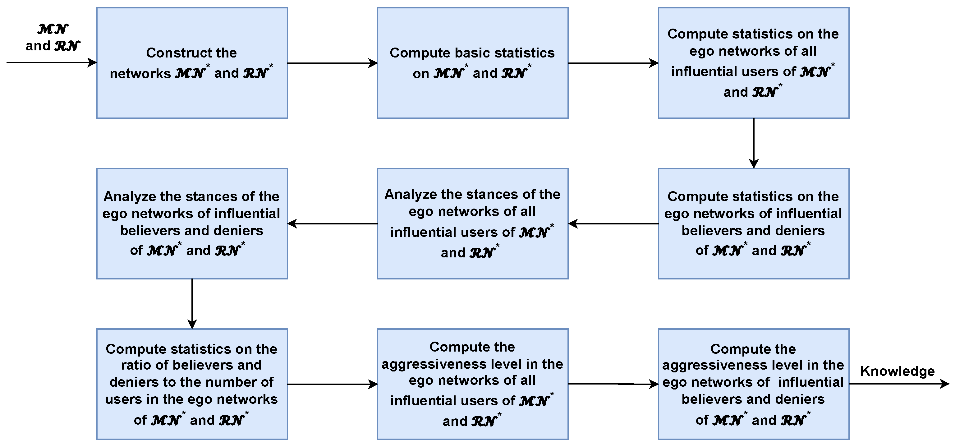
Figure 17 illustrates the workflow we followed to determine the polarization level of the most influential users in $\mathcal{MN}$ and $\mathcal{RN}$. As shown in the figure, we first constructed the networks ${\mathcal{MN}}^{*}$ and ${\mathcal{RN}}^{*}$ by identifying the most influential users in $\mathcal{MN}$ and $\mathcal{RN}$, constructing the corresponding ego networks and integrating the latter. Once ${\mathcal{MN}}^{*}$ and ${\mathcal{RN}}^{*}$ were obtained, we calculated various basic statistics on them. Then, we computed statistics on the ego networks of all influential users in ${\mathcal{MN}}^{*}$ and ${\mathcal{RN}}^{*}$ and compared them with the corresponding statistics on the ego networks of influential believers and deniers in the same networks. Next, we analyzed the stances inside the ego networks of all influential users in ${\mathcal{MN}}^{*}$ and ${\mathcal{RN}}^{*}$ and compared them with the stances of the influential believers and deniers in the same networks. Afterward, we calculated some statistics on the ratio $r_b$ (resp., $r_d$) of the number of believers (resp., deniers) to the number of users in the ego networks of ${\mathcal{MN}}^{*}$ and ${\mathcal{RN}}^{*}$. Finally, we calculated the aggressiveness level in the ego networks of all influential users in ${\mathcal{MN}}^{*}$ and ${\mathcal{RN}}^{*}$ and compared it with the aggressiveness level in the ego networks of influential believers and deniers in the same networks. Each of these tasks provided insights into the characteristics of influential users in $\mathcal{MN}$ and $\mathcal{RN}$. Below, we illustrate each step of the workflow in detail.

The first step in studying the polarization of influential users was to construct the networks ${\mathcal{MN}}^{*}$ and ${\mathcal{RN}}^{*}$ (see Equation (8)) corresponding to $\mathcal{MN}$ and $\mathcal{RN}$. Recall that ${\mathcal{MN}}^{*}$ (resp., ${\mathcal{RN}}^{*}$) is the subnetwork of $\mathcal{MN}$ (resp., $\mathcal{RN}$) obtained by merging the ego networks of the top T users for each possible stance of $\mathcal{S}$ (see Section 3.3.2). In our dataset, we have 2 possible stances, namely “believer” and “denier”; furthermore, we set $T=1500$. As a consequence ${\mathcal{MN}}^{*}$ and ${\mathcal{RN}}^{*}$ are constructed by merging the ego networks of the top 3000 influential users of $\mathcal{MN}$ and $\mathcal{RN}$, respectively. In Section 4.4.4, we illustrate an experiment regarding the tuning of T.

The first statistics we calculated are the number of nodes, the number of edges and the density of the two networks. The results obtained are shown in

Table 12. Some statistics of ${\mathcal{MN}}^{*}$ and ${\mathcal{RN}}^{*}$.

Statistic	${\mathcal{MN}}^{*}$	${\mathcal{RN}}^{*}$
Number of nodes	49,894	35,828
Number of edges	103,875	53,894
Density	8346·10−5	8.397·10−5

. From the analysis of this table, we can observe that ${\mathcal{MN}}^{*}$ has a greater number of nodes and edges than ${\mathcal{RN}}^{*}$; this implies that the ego networks of ${\mathcal{MN}}^{*}$ are, on average, larger than the ones of ${\mathcal{RN}}^{*}$. In contrast, the density of the two networks is approximately the same. This result can be justified considering the statistics of the networks $\mathcal{MN}$ and $\mathcal{RN}$, from which ${\mathcal{MN}}^{*}$ and ${\mathcal{RN}}^{*}$ are derived (see Table 6). They indicate that the number of nodes and edges in $\mathcal{MN}$ is higher than in $\mathcal{RN}$, while the density of the two networks is comparable.

4.4.1. Analysis of the Ego Networks of All Users

At this point, we focused on the individual ego networks associated with the 3000 most influential users that gave rise to ${\mathcal{MN}}^{*}$ (resp., ${\mathcal{RN}}^{*}$). To this end, for each ego network, we calculated the values of a set of statistics and, then, the corresponding means and variances. The results obtained are shown in

Table 13. Mean and variance of the values of some statistics for the ego networks in ${\mathcal{MN}}^{*}$ and ${\mathcal{RN}}^{*}$.

Statistic	Mean in ${\mathcal{MN}}^{*}$	Variance in ${\mathcal{MN}}^{*}$	Mean in ${\mathcal{RN}}^{*}$	Variance in ${\mathcal{RN}}^{*}$
Number of nodes	45.324	189.943	22.467	174.321
Number of edges	153.125	443.454	26.235	182.458
Density	0.262	0.231	0.228	0.172
Average sentiment	0.013	0.196	−0.070	0.167
Average number of aggressive tweets	30.965	42.176	19.005	46.443
Average number of non-aggressive tweets	104.765	171.375	61.496	235.485
Average number of believers	12.374	25.358	3.932	6.365
Average number of deniers	5.521	15.284	1.792	4.473
Average clustering coefficient	0.315	0.228	0.109	0.159

.

From the analysis of this table, we can see that the ego networks of ${\mathcal{MN}}^{*}$ are larger in terms of number of nodes and edges than the ego networks of ${\mathcal{RN}}^{*}$. The densities of the two categories of ego networks are comparable (i.e., 0.262 vs. 0.228). Again, this can be explained by looking at the statistics of $\mathcal{MN}$ and $\mathcal{RN}$ shown in Table 6. In terms of sentiment, the ego networks of ${\mathcal{MN}}^{*}$ have a moderately positive average sentiment while the average sentiment of the ego networks of ${\mathcal{RN}}^{*}$ is moderately negative. When examining the content, it can be seen that both the average number of aggressive tweets and the average number of non-aggressive tweets are higher in the ego networks of ${\mathcal{MN}}^{*}$ than in the ego networks of ${\mathcal{RN}}^{*}$. However, the ratio of the average number of aggressive tweets to the average number of non-aggressive tweets is approximately equal in both types of ego networks (i.e., 0.2956 vs. 0.3090). The average number of believers and deniers is always higher in the ego networks of ${\mathcal{MN}}^{*}$ than in the ego network of ${\mathcal{RN}}^{*}$. However, the polarization ratio, computed by applying Equation (12), is comparable in the two types of ego networks (i.e., 2.2412 vs. 2.1942). These results can be explained by the fact that the size of $\mathcal{MN}$ is much larger than the one of $\mathcal{RN}$. This implies that many more users (and proportionally many more believers and deniers) are active in $\mathcal{MN}$ than in $\mathcal{RN}$. The fact that the ratio of user stances and the ratio of aggressive to non-aggressive tweets are similar in ${\mathcal{MN}}^{*}$ and ${\mathcal{RN}}^{*}$ is a further confirmation that the higher numbers in ${\mathcal{MN}}^{*}$ are due solely to the larger size of $\mathcal{MN}$.

One of the most interesting data points from this first set of statistics concerns the value of the average clustering coefficient. Recall that this is a measure of how much the alters of an ego network tend to connect with each other, in addition to being connected with the corresponding ego. The average clustering coefficient is considerably higher in the ego networks of ${\mathcal{MN}}^{*}$ than in the ego networks of ${\mathcal{RN}}^{*}$ (i.e., 0.315 vs. 0.109). This indicates that the nodes in the ego networks of ${\mathcal{MN}}^{*}$ are likely to be more interconnected than the nodes in the ego networks of ${\mathcal{RN}}^{*}$. This can be explained by taking into account the different dynamics of mentioning and replying that generally occur on X, where replying activity is concentrated on a smaller number of messages that stimulate debate, whereas mentioning is more distributed across multiple tweets and users. In particular, it is quite common for many replies to refer to the same starting tweet. This favors a star configuration of the subnetwork of users involved, where the star center is the user who made the initial tweet to which everyone is replying. A star configuration results in many open triads and thus a low clustering coefficient [73]. Instead, mentioning is distributed over multiple messages and multiple users, with frequent “transitive” transitions (i.e., a user A mentions a user B who mentions a user C who may have been mentioned by A). This favors a much denser configuration of the subnetwork of users involved and thus the presence of many closed triads, which favors a higher clustering coefficient.

4.4.2. Analysis of the Ego Networks of Believers and Deniers

After computing a set of statistics for the ego networks of all users, regardless of the stance they follow, we decided to recalculate the same statistics but partitioning users according to their stance. The goal of this activity is to make a comparison between the different stances of users by checking whether there are differences in their behavior. Specifically, in

Table 14. Mean and variance of the values of some statistics for the ego networks of believers in ${\mathcal{MN}}^{*}$ and ${\mathcal{RN}}^{*}$.

Statistic	Mean in ${\mathcal{MN}}^{*}$	Variance in ${\mathcal{MN}}^{*}$	Mean in ${\mathcal{RN}}^{*}$	Variance in ${\mathcal{RN}}^{*}$
Number of nodes	28.634	321.127	13.834	302.189
Number of edges	117.589	685.323	15.976	308.143
Density	0.68	0.168	0.053	0.170
Average sentiment	0.022	0.134	−0.014	0.139
Average number of aggressive tweets	17.298	42.843	7.101	38.224
Average number of non-aggressive tweets	58.234	155.743	20.698	168.342
Average number of believers	10.598	36.265	2.732	8.178
Average number of deniers	1.210	13.321	0.741	6.548
Average clustering coefficient	0.481	0.178	0.041	0.141

(resp.,

Table 15. Mean and variance of the values of some statistics for the ego networks of deniers in ${\mathcal{MN}}^{*}$ and ${\mathcal{RN}}^{*}$.

Statistic	Mean in ${\mathcal{MN}}^{*}$	Variance in ${\mathcal{MN}}^{*}$	Mean in ${\mathcal{RN}}^{*}$	Variance in ${\mathcal{RN}}^{*}$
Number of nodes	9.352	33.634	4.701	16.575
Number of edges	23.82	211.789	5.124	24.212
Density	0.066	0.168	0.073	0.156
Average sentiment	−0.031	0.115	−0.036	0.147
Average number of aggressive tweets	7.198	32.856	4.243	37.097
Average number of non-aggressive tweets	22.098	149.043	13.498	182.201
Average number of believers	1.187	3.765	0.749	2.597
Average number of deniers	3.069	19.401	0.725	4.111
Average clustering coefficient	0.202	0.224	0.033	0.098

) we show the mean and variance of the same parameters seen in Table 13 but for believers (resp., deniers) only.

From the analysis of these two tables, we first observe that the ego networks of believers tend to be more populated than those of deniers. This trend is noticeable on the ego networks of both ${\mathcal{MN}}^{*}$ and ${\mathcal{RN}}^{*}$. It can be explained by the distribution of believers and deniers in the networks $\mathcal{MN}$ and $\mathcal{RN}$ (see Table 9) from which the networks ${\mathcal{MN}}^{*}$ and ${\mathcal{RN}}^{*}$ are derived. This trend allows us to infer that believers have a greater tendency to generate discussions on climate change than deniers.

As a next analysis, we decided to assess the stances of the users belonging to the ego networks of believers and deniers in ${\mathcal{MN}}^{*}$ and ${\mathcal{RN}}^{*}$. Regarding the ego networks of believers (Table 14) we note that the average number of believers in them is much greater than the average number of deniers. This trend is very marked in ${\mathcal{MN}}^{*}$, where the polarization ratio $r_{bd}$ is 8.76 (recall that $r_{bd}=2.2412$ in ${\mathcal{MN}}^{*}$ and $r_{bd}=2.1942$ in ${\mathcal{RN}}^{*}$). The same trend can be observed in ${\mathcal{RN}}^{*}$, albeit it is less marked (in particular, the value of $r_{bd}$ is 3.69 in this case). Regarding the ego networks of deniers (Table 15), we can observe that the polarization ratio $r_{bd}$ is equal to 0.39 in ${\mathcal{MN}}^{*}$ and to 1.03 in ${\mathcal{RN}}^{*}$. This polarization result is even more important if we consider that the starting dataset and the corresponding network $\mathcal{N}$ are strongly skewed toward believers. Indeed, despite the huge presence of believers, we still observe more deniers in ${\mathcal{MN}}^{*}$ and approximately the same number of believers and deniers in ${\mathcal{RN}}^{*}$. Consequently, we can conclude that, in believers, there is a strong polarization in ${\mathcal{MN}}^{*}$ and a polarization in ${\mathcal{RN}}^{*}$, in both cases in favor of believers. Polarization is also observed among deniers, but in favor of deniers in ${\mathcal{MN}}^{*}$ while no significant polarization can be observed in ${\mathcal{RN}}^{*}$. As mentioned above, the polarization found can be explained by the fact that polarized communities are closed and their members communicate mainly to reinforce their beliefs [52]. In this type of groups, people generally do not want to expose themselves outside their community, and tend to be reactive rather than proactive [19,74].

As a further analysis on polarization, we considered the ratio of the average number of believers and deniers to the number of nodes for the ego networks of ${\mathcal{MN}}^{*}$ and ${\mathcal{RN}}^{*}$. We call these ratios $r_b$ and $r_d$ in the following. In

Table 16. Values of $r_b$ and $r_d$ for the ego networks of believers and deniers in ${\mathcal{MN}}^{*}$ and ${\mathcal{RN}}^{*}$.

Network	${\mathit{r}}_{\mathit{b}}$	${\mathit{r}}_{\mathit{d}}$
ego networks of believers
${\mathcal{MN}}^{*}$	0.361	0.041
${\mathcal{RN}}^{*}$	0.201	0.054
ego networks of deniers
${\mathcal{MN}}^{*}$	0.124	0.318
${\mathcal{RN}}^{*}$	0.161	0.156

, we report the values of these ratios for the ego networks of believers and deniers in both ${\mathcal{MN}}^{*}$ and ${\mathcal{RN}}^{*}$. The analysis in this table fully confirms the previous results. In fact, as for the ego networks of believers, there is an extremely higher value of $r_b$ than $r_d$ in ${\mathcal{MN}}^{*}$ and a higher value of $r_b$ than $r_d$ in ${\mathcal{RN}}^{*}$. In contrast, as for the ego networks of deniers, there is quite a higher value of $r_d$ than $r_b$ in ${\mathcal{MN}}^{*}$, while the values of $r_b$ and $r_d$ are approximately the same in ${\mathcal{RN}}^{*}$. Interestingly, as for the ego networks of ${\mathcal{MN}}^{*}$ the value of $r_b$ in the ego networks of believers and that of $r_d$ in the ego networks of deniers are close. As for the ego networks of ${\mathcal{RN}}^{*}$, only the value of $r_b$ for the ego networks of believers is significantly greater than the value of $r_d$, while the two values are similar for the ego networks of deniers. Therefore, this analysis confirms that the ego networks of ${\mathcal{RN}}^{*}$ are less polarized than those of ${\mathcal{MN}}^{*}$ and this polarization only affects believers.

Returning to Table 14 and Table 15, an interesting observation concerns the average clustering coefficient. In fact, we can see that, in ${\mathcal{MN}}^{*}$ the average clustering coefficient of the ego networks of believers is high whereas that of the ego network of deniers is medium. Instead, in ${\mathcal{RN}}^{*}$ the average clustering coefficient of believers and deniers is low. Recall that the clustering coefficient indicates the tendency of the alters to communicate with each other besides their ego. Therefore, a high clustering coefficient is a further confirmation of the polarization phenomenon involving believers, and partially deniers, in ${\mathcal{MN}}^{*}$. As for ${\mathcal{RN}}^{*}$, there is a slightly higher value of the average clustering coefficient for the ego networks of believers than the ones of deniers, and this is a further confirmation of the polarization results we had identified for ${\mathcal{RN}}^{*}$ in the previous analyses.

4.4.3. Analysis of the Aggressiveness Level of the Tweets in the Ego Networks of Believers and Deniers

Proceeding with our investigation, we analyzed the aggressiveness level of the tweets in the ego networks of believers and deniers. To conduct this study, we calculated the ratio $r_a$ of the average number of aggressive tweets to the average number of non-aggressive tweets in the two types of ego networks in both ${\mathcal{MN}}^{*}$ and ${\mathcal{RN}}^{*}$. The results obtained are shown in

Table 17. Values of $r_a$ for the ego networks of believers and deniers in ${\mathcal{MN}}^{*}$ and ${\mathcal{RN}}^{*}$.

Network	${\mathit{r}}_{\mathit{a}}$ in ${\mathcal{MN}}^{*}$	${\mathit{r}}_{\mathit{a}}$ in ${\mathcal{RN}}^{*}$
Ego networks of believers	0.298	0.343
Ego networks of deniers	0.326	0.314

.

From the analysis of this table, we can observe that in ${\mathcal{MN}}^{*}$ the ego networks of deniers have a slightly higher aggressiveness level than the ego networks of believers. In contrast, in ${\mathcal{RN}}^{*}$, the ego networks of believers have a slightly higher aggressiveness level than the ego networks of deniers but the aggressiveness level of deniers is still high. The increased aggressiveness of deniers, observed in both ${\mathcal{MN}}^{*}$ and ${\mathcal{RN}}^{*}$, is a confirmation of the sociological findings that climate deniers exhibit aggressive attitudes [12,75,76]. Interestingly, the way of proceeding we took to reach this conclusion is very different from the methods generally used by sociologists to reach it. The orthogonality of approaches provides greater certainty about the conclusions they reach and strengthens them both. Believer aggressiveness is found more in ${\mathcal{RN}}^{*}$ than in ${\mathcal{MN}}^{*}$, and this can be explained by taking into account what we said above about the fact that, when replying, one chooses the message and also knows the ideas of its sender. Being a closed community, and also having the opportunity to choose the interlocutor (who is most likely already known), one can be much more direct in expressing her thoughts by dropping inhibitions, which favors an increase in the aggressiveness with which she expresses her thoughts.

4.4.4. Analysis of the Appropriateness of the Chosen Value of T

In Section 4.4, we chose a value of T equal to 1500, which means that we examined the top 1500 believers and the top 1500 deniers. In total, our network ${\mathcal{N}}^{*}$ is based on 3000 influential users and thus on the fusion of 3000 ego networks. This number seems extremely low, since it is 0.23% of all users. However, this is due to the fact that we wanted to take the top influential users, and we saw that the power law distributions in Figure 8 and Figure 9 are extremely steep, as evidenced by the values of a reported in Section 4.2. However, we would like to point out that, starting from these values, we obtain a network ${\mathcal{MN}}^{*}$ whose number of users is equal to 49,894, i.e., 3.97% of the users of the original network $\mathcal{MN}$. Similarly, the network ${\mathcal{RN}}^{*}$ consists of 35,828 users, i.e., 12.21% of the users of the original network $\mathcal{RN}$. In our opinion, a lower value of T would risk generating networks, and therefore analyses, which are not very significant.

One could ask if the chosen value of T is too small to be significant or if it is sufficient. To answer this question, we decided to consider higher values of T. In particular, we considered $T=3000$, $T=5000$, $T=10,000$, and $T=20,000$. For each of these values, we calculated the same parameters as in Table 12 and Table 13. The results obtained are shown in

Table 18. Some statistics of ${\mathcal{MN}}^{*}$ and ${\mathcal{RN}}^{*}$ for different values of T.

Statistic	${\mathcal{MN}}^{*}$	${\mathcal{RN}}^{*}$
T = 1500
Number of nodes	49,894	35,828
Number of edges	103,875	53,894
Density	8346·10−5	8.397·10−5
T = 3000
Number of nodes	111,675	74,734
Number of edges	412,923	238,195
Density	6622·10−5	8.530·10−5
T = 5000
Number of nodes	184,486	123,934
Number of edges	723,538	521,584
Density	4252·10−5	6.792·10−5
T = 10,000
Number of nodes	326,936	206,376
Number of edges	1,325,734	984,038
Density	2.482·10−5	4621·10−5
T = 20,000
Number of nodes	584,194	398,240
Number of edges	2,421,947	1,723,484
Density	1.419·10−5	2.173·10−5

and

Table 19. Mean and variance of the values of some statistics for the ego networks in ${\mathcal{MN}}^{*}$ and ${\mathcal{RN}}^{*}$ for different values of T.

textbfStatistic	Mean in ${\mathcal{MN}}^{*}$	Variance in ${\mathcal{MN}}^{*}$	Mean in ${\mathcal{RN}}^{*}$	Variance in ${\mathcal{RN}}^{*}$
T = 1000
Number of nodes	44.324	189.943	22.467	174.321
Number of edges	153.125	443.454	26.235	182.458
Density	0.262	0.231	0.228	0.172
Average sentiment	0.013	0.196	−0.070	0.167
Average number of aggressive tweets	30.965	42.176	19.005	46.443
Average number of non-aggressive tweets	104.765	171.375	61.496	235.485
Average number of believers	12.374	25.358	3.932	6.365
Average number of deniers	5.521	15.284	1.792	4.473
Average clustering coefficient	0.315	0.228	0.109	0.159
T = 3000
Number of nodes	43.834	201.276	21.985	190.321
Number of edges	152.236	446.296	25.756	188.539
Density	0.251	0.281	0.226	0.192
Average sentiment	0.014	0.220	−0.068	0.194
Average number of aggressive tweets	29.243	48.155	20.432	54.224
Average number of non-aggressive tweets	103.265	182.238	60.947	236.345
Average number of believers	11.845	28.275	4.184	8.998
Average number of deniers	5.025	19.995	1.653	6.007
Average clustering coefficient	0.314	0.258	0.111	0.189
T = 5000
Number of nodes	44.538	205.639	22.364	193.735
Number of edges	153.395	463.037	26.007	192.343
Density	0.241	0.281	0.227	0.192
Average sentiment	0.015	0.220	−0.065	0.198
Average number of aggressive tweets	30.284	52.690	19.003	57.012
Average number of non-aggressive tweets	104.103	193.107	61.496	243.369
Average number of believers	12.048	32.395	4.385	10.952
Average number of deniers	5.194	22.952	1.229	8.285
Average clustering coefficient	0.294	0.328	0.121	0.219
T = 10,000
Number of nodes	44.749	208.265	22.740	198.101
Number of edges	151.374	673.285	23.295	196.375
Density	0.251	0.281	0.236	0.192
Average sentiment	0.013	0.245	−0.070	0.221
Average number of aggressive tweets	28.264	55.386	19.409	59.495
Average number of non-aggressive tweets	104.395	198.285	59.090	247.308
Average number of believers	10.908	34.006	4.506	12.375
Average number of deniers	5.432	25.658	1.258	10.497
Average clustering coefficient	0.304	0.321	0.121	0.234
T = 20,000
Number of nodes	43.638	214.259	23.047	201.285
Number of edges	150.285	679.222	24.465	202.089
Density	0.241	0.321	0.226	0.221
Average sentiment	0.014	0.264	−0.069	0.234
Average number of aggressive tweets	27.285	58.887	20.994	61.438
Average number of non-aggressive tweets	103.295	210.480	60.184	253.158
Average number of believers	11.205	36.375	5.298	13.002
Average number of deniers	4.859	27.320	1.264	12.376
Average clustering coefficient	0.294	0.367	0.119	0.289

.

From the analysis of these tables we can see that the means of the different measures do not change significantly compared to the case in which $T=1500$, while the variances increase. Therefore, increasing T does not lead to significant variations of extracted information, and, at the same time, it leads to longer computation times and greater variance in the results. For all these reasons, we believe that the value $T=1500$ is the best one for our analysis of influential users.

5. Discussion

In this section, we present a discussion on the proposed framework that also takes into account the results of our experimental campaign. In particular, in Section 5.1 we illustrate the implications of our framework. In Section 5.2, we present some of its limitations. Finally, in Section 5.3 we show how our framework can be extended to include the time dimension.

5.1. Implications

The results of our experiments showed that our framework can assess the polarization level of communities and influential users discussing climate change on X. Through community analysis, we found that mention and reply relationships tend to create unbalanced communities, where users are mainly believers or deniers. Next, the analysis of the ego networks of influential users reported that users with similar views tend to cluster together, which shows that the homophily property [73] characterizes these types of users. Although we tested our framework on X, we emphasize that our proposal is generic and can be applied to any OSN. In fact, our framework allows us to study polarization in any scenario characterized by users who publish comments that generally highlight a well-determined stance with respect to a general topic.

In addition to the results of our experiments, our framework has many other interesting implications. For example, we could assess how controversial a topic is by calculating how much polarized users discussing it are. Moreover, we can study how the polarization of communities or influential users varies over time by also trying to understand the reasons leading to variations (see Section 5.3 for more details).

Furthermore, our framework can enable us to carry out investigations on issues other than polarization although related to it. For example, it could allow us to analyze the spread of fake news within a polarized community and how it contributes to reinforce the opinions of its users [25]. This phenomenon damages the general discussion on a topic because of the diffusion of false claims and/or facts without any scientific basis. Another implication concerns the recommendation of content to users, which plays a key role in the polarization of OSNs and the creation of echo chambers [77]. In this context, if through our framework we verify the presence of polarization in some communities, we can think of adapting the content proposed to users in them in such a way as to stimulate their exploration of other points of view. In this way, we could hope to mitigate the harm of polarization and create healthier discussions.

An important consideration should be made about the network ${\mathcal{N}}^{*}$. In fact, it is obtained by integrating the ego networks of the most influential users. Therefore, there is a possibility that it could be disconnected. Consequently, the networks ${\mathcal{MN}}^{*}$ and ${\mathcal{RN}}^{*}$ could in principle also be disconnected. However, this does not affect the validity of the different measures that we considered in Section 4.4, and therefore the results of the corresponding analyses. In fact, none of these measures assumes that the network on which they are calculated is connected.

5.2. Limitations

Our framework also presents some limitations. The first concerns the need to have user stances as input. In our experiments, we adopted the dataset of [33] that provided this information. In other cases, we would have had to extract user stances exploiting Natural Language Processing algorithms (similar to what the authors of [33] did before publishing their dataset).

The second limitation concerns the fact that our framework requires a quite large dataset of comments/posts to measure the polarization level of an OSN. Actually, this limitation can be accepted because our framework was designed to operate offline and not in real time (see Section 4.3.1 for more details).

5.3. A Possible Extension Toward Time Modeling

Our framework is currently static. Given a topic of interest and an OSN where it is discussed, it considers all comments exchanged within the OSN during a specified time interval and determines whether the communities and the most influential users of the OSN are polarized. It is not currently able to determine how phenomena related to polarization vary over time. However, we can carry out a simple dynamic extension of our framework to handle the time dimension, without disrupting the algorithms that define its current behavior. In this section, we provide an overview of how this can be achieved.

The first fundamental extension to consider is the modeling of time. In this case, we can think of a discrete modeling of this measure. Given a time interval T, it is possible to divide it into subintervals of length $\Delta t$. Let z be the number of these subintervals. For each subinterval t, $1\le t\le z$, we can construct a network:

$${\mathcal{N}}_t=\langle N_t,E_t\rangle$$

(14)

analogous to the network $\mathcal{N}$ defined in Equation (1). Starting from ${\mathcal{N}}_t$, we can obtain all the data structures defined in Equations (6)–(11). Applying the Louvain algorithm to ${\mathcal{N}}_t$ determines the set $Q_t$ of communities present in ${\mathcal{N}}_t$. Similarly, we can determine the polarization ratio $r_{b{d}_t}$ (Equation 12), the fraction $r_{b_t}$ of believers and the fraction $r_{d_t}$ of deniers in ${\mathcal{N}}_t$ (see Section 4.4.2), as well as the ratio $r_{a_t}$ between aggressive and non-aggressive comments in ${\mathcal{N}}_t$ (see Section 4.4.3). The subscript t in each of these parameters indicates that they are calculated with reference to the time interval t.

This gives us a set of time series, one for each parameter mentioned above. We can then apply all the approaches and indices provided in time series theory to extract dynamic information about polarization in an OSN. For instance, we can perform:

• Basic analyses, such as identifying the maximum, minimum, mean, standard deviation, trend and spikes.
• Event alignment analyses, aimed to identify temporal correlation between exogenous phenomena (such as political announcements, or extreme events) and changes in communities or corresponding polarization indices within the reference OSN.
• Early warning analyses, which identify the initial signs preceding certain phenomena, such as community splitting, echo chamber consolidation, the reduction, or even disappearance, of the polarization level of a community, etc.

As this simple description shows, extending our framework to include the time dimension does not affect the basic algorithms that determine the functioning of our framework. Therefore, it can be done without enormous effort. At the same time, as demonstrated by the above examples (and many others that could be thought of), the amount of additional knowledge that can be detected is significant.

6. Conclusions

In this paper, we have presented a framework for investigating the polarization phenomenon on an OSN. Starting with a dataset of comments on a specific topic, our framework creates a network of user interactions and then exploits this network, and other ones derived from it, to analyze the polarization of communities and influential users on that topic. To validate our framework, we leveraged an X dataset containing tweets related to climate change. Thanks to our framework, we could see that there is a strong polarization of both communities and influential users on this topic. In fact, we have seen that the communities of believers and deniers are mostly made up of like-minded people and that influential users tend to surround themselves with other users having similar points of view.

In the future, we plan to continue this research in several directions. For example, we can think of analyzing the media (emoticons, images, videos) attached to a comment, which could reveal us additional insights regarding the polarization of communities and influential users. Furthermore, we aim to consider more kinds of user interaction at a time. This holistic approach would allow us to investigate the nuances of online conversations and engagements more closely. For instance, the frequency and context of likes and shares can offer insights into silent endorsements or passive agreement within communities. Additionally, examining the patterns of retweets can help identify the pathways through which polarizing content is disseminated and how it influences the network at large. In this way, we could determine the overall polarization of communities and users within an OSN, which could be employed for improving the user experience on it. Finally, we think that the knowledge extracted through our framework could be employed in a Graph Neural Network model to predict the next users and posts with which a person will interact based on her polarization level and the content she posted.

References

1. Baym, N.K. Personal Connections in the Digital Age; John Wiley & Sons: Hoboken, NJ, USA, 2015. [Google Scholar]
2. Bonifazi, G.; Corradini, E.; Marchetti, M.; Sciarretta, L.; Ursino, D.; Virgili, L. A Space-Time Framework for Sentiment Scope Analysis in Social Media. Big Data Cogn. Comput. 2022, 6, 130. [Google Scholar] [CrossRef]
3. Wu, W.; Weaver, D. On-line democracy or on-line demagoguery? Public opinion “polls” on the Internet. Harv. Int. J. Press. 1997, 2, 71–86. [Google Scholar] [CrossRef]
4. Chang, H.; Tsai, F. A Systematic Review of Internet Public Opinion Manipulation. Procedia Comput. Sci. 2022, 207, 3159–3166. [Google Scholar] [CrossRef]
5. Qais, A. The Internet and Its Impact on Free Speech. Indian J. Law Leg. Res. 2023, 5, 1. [Google Scholar]
6. Stoner, J. Risky and cautious shifts in group decisions: The influence of widely held values. J. Exp. Soc. Psychol. 1968, 4, 442–459. [Google Scholar] [CrossRef]
7. Bonifazi, G.; Breve, B.; Cirillo, S.; Corradini, E.; Virgili, L. Investigating the COVID-19 vaccine discussions on Twitter through a multilayer network-based approach. Inf. Process. Manag. 2022, 59, 103095. [Google Scholar] [CrossRef]
8. Casañ, R.; García-Vidal, E.; Grimaldi, D.; Carrasco-Farré, C.; Vaquer-Estalrich, F.; Vila-Francés, J. Online polarization and cross-fertilization in multi-cleavage societies: The case of Spain. Soc. Netw. Anal. Min. 2022, 12, 79. [Google Scholar] [CrossRef]
9. Cantini, R.; Marozzo, F.; Talia, D.; Trunfio, P. Analyzing political polarization on social media by deleting bot spamming. Big Data Cogn. Comput. 2022, 6, 3. [Google Scholar] [CrossRef]
10. McPherson, M.; Smith-Lovin, L.; Cook, J. Birds of a feather: Homophily in social networks. Annu. Rev. Sociol. 2001, 27, 415–444. [Google Scholar] [CrossRef]
11. Lazarsfeld, P.; Merton, R. Friendship as a social process: A substantive and methodological analysis. Freedom Control Mod. Soc. 1954, 18, 18–66. [Google Scholar]
12. Cinelli, M.; Pelicon, A.; Mozetič, I.; Quattrociocchi, W.; Novak, P.; Zollo, F. Dynamics of online hate and misinformation. Sci. Rep. 2021, 11, 1–12. [Google Scholar] [CrossRef]
13. Enjolras, B.; Salway, A. Homophily and polarization on political twitter during the 2017 Norwegian election. Soc. Netw. Anal. Min. 2022, 13, 10. [Google Scholar] [CrossRef]
14. Borah, A.; Singh, S. Investigating political polarization in India through the lens of Twitter. Soc. Netw. Anal. Min. 2022, 12, 97. [Google Scholar] [CrossRef]
15. Belaroussi, R.; Noufe, S.C.; Dupin, F.; Vandanjon, P.O. Polarity of Yelp Reviews: A BERT–LSTM Comparative Study. Big Data Cogn. Comput. 2025, 9, 140. [Google Scholar] [CrossRef]
16. Mäs, M.; Flache, A. Differentiation without distancing. Explaining bi-polarization of opinions without negative influence. PLoS ONE 2013, 8, e74516. [Google Scholar] [CrossRef]
17. Van Houtte, M. School type and academic culture: Evidence for the differentiation–polarization theory. J. Curric. Stud. 2006, 38, 273–292. [Google Scholar] [CrossRef]
18. Min, Y.; Jiang, T.; Jin, C.; Li, Q.; Jin, X. Endogenetic structure of filter bubble in social networks. R. Soc. Open Sci. 2019, 6, 190868. [Google Scholar] [CrossRef] [PubMed]
19. Chitra, U.; Musco, C. Analyzing the impact of filter bubbles on social network polarization. In Proceedings of the International Conference on Web Search and Data Mining (WSDM’20), Houston, TX, USA, 3–7 February 2020; pp. 115–123. [Google Scholar]
20. Schmidt, A.L.; Zollo, F.; Scala, A.; Betsch, C.; Quattrociocchi, W. Polarization of the vaccination debate on Facebook. Vaccine 2018, 36, 3606–3612. [Google Scholar] [CrossRef]
21. Moernaut, R.; Mast, J.; Temmerman, M.; Broersma, M. Hot weather, hot topic. Polarization and sceptical framing in the climate debate on Twitter. Inf. Commun. Soc. 2022, 25, 1047–1066. [Google Scholar] [CrossRef]
22. Garimella, K.; Morales, G.D.F.; Gionis, A.; Mathioudakis, M. Political discourse on social media: Echo chambers, gatekeepers, and the price of bipartisanship. In Proceedings of the World Wide Web Conference (WWW’18), Lyon, France, 23–27 April 2018; pp. 913–922. [Google Scholar]
23. Conover, M.; Ratkiewicz, J.; Francisco, M.; Gonçalves, B.; Menczer, F.; Flammini, A. Political polarization on Twitter. In Proceedings of the International AAAI Conference on Web and Social Media (ICWSM’11), Barcelona, Spain, 17–21 July 2011; Volume 5, pp. 89–96. [Google Scholar]
24. Li, L.; Scaglione, A.; Swam, A.; Zhao, Q. Consensus, polarization and clustering of opinions in social networks. IEEE J. Sel. Areas Commun. 2013, 31, 1072–1083. [Google Scholar] [CrossRef]
25. Baumann, F.; Lorenz-Spreen, P.; Sokolov, I.; Starnini, M. Modeling echo chambers and polarization dynamics in social networks. Phys. Rev. Lett. 2020, 124, 048301. [Google Scholar] [CrossRef]
26. Arora, S.; Singh, G.; Chakraborty, A.; Maity, M. Polarization and social media: A systematic review and research agenda. Technol. Forecast. Soc. Change 2022, 183, 121942. [Google Scholar] [CrossRef]
27. Hajibagheri, A.; Sukthankar, G. Political Polarization Over Global Warming: Analyzing Twitter Data on Climate Change; Academy of Science and Engineering (ASE): Los Angeles, CA, USA, 2014. [Google Scholar]
28. Overgaard, C.; Woolley, S. How Social Media Platforms Can Reduce Polarization; Technical report; Brookings Institution: Washington, DC, USA, 2022. [Google Scholar]
29. Xie, L.; Wang, D.; Ma, F. Analysis of individual characteristics influencing user polarization in COVID-19 vaccine hesitancy. Comput. Hum. Behav. 2023, 143, 107649. [Google Scholar] [CrossRef]
30. Tyagi, A.; Uyheng, J.; Carley, K. Affective polarization in online climate change discourse on twitter. In Proceedings of the IEEE/ACM International Conference on Advances in Social Networks Analysis and Mining (ASONAM ’20), IEEE, Virtual Event, 7–10 December 2020; pp. 443–447. [Google Scholar]
31. Musco, C.; Musco, C.; Tsourakakis, C.E. Minimizing polarization and disagreement in social networks. In Proceedings of the World Wide Web conference (WWW’18), Lyon, France, 23–27 April 2018; pp. 369–378. [Google Scholar]
32. Chen, X.; Lijffijt, J.; Bie, T.D. Quantifying and minimizing risk of conflict in social networks. In Proceedings of the ACM SIGKDD International Conference on Knowledge Discovery & Data Mining (KDD’18), London, UK, 19–23 August 2018; pp. 1197–1205. [Google Scholar]
33. Effrosynidis, D.; Karasakalidis, A.; Sylaios, G.; Arampatzis, A. The climate change Twitter dataset. Expert Syst. Appl. 2022, 204, 117541. [Google Scholar] [CrossRef]
34. Tucker, J.; Guess, A.; Barberá, P.; Vaccari, C.; Siegel, A.; Sanovich, S.; Stukal, D.; Nyhan, B. Social media, political polarization, and political disinformation: A review of the scientific literature. SSRN Electron. J. 2018. [Google Scholar] [CrossRef]
35. Falkenberg, M.; Galeazzi, A.; Torricelli, M.; Marco, N.D.; Larosa, F.; Sas, M.; Mekacher, A.; Pearce, W.; Zollo, F.; Quattrociocchi, W. Growing polarization around climate change on social media. Nat. Clim. Change 2022, 12, 1114–1121. [Google Scholar] [CrossRef]
36. Matakos, A.; Terzi, E.; Tsaparas, P. Measuring and moderating opinion polarization in social networks. Data Min. Knowl. Discov. 2017, 31, 1480–1505. [Google Scholar] [CrossRef]
37. Sikder, O.; Smith, R.; Vivo, P.; Livan, G. A minimalistic model of bias, polarization and misinformation in social networks. Sci. Rep. 2020, 10, 5493. [Google Scholar] [CrossRef]
38. Gruzd, A.; Roy, J. Investigating political polarization on Twitter: A Canadian perspective. Policy Internet 2014, 6, 28–45. [Google Scholar] [CrossRef]
39. Lee, C.; Shin, J.; Hong, A. Does social media use really make people politically polarized? Direct and indirect effects of social media use on political polarization in South Korea. Telemat. Inform. 2018, 35, 245–254. [Google Scholar] [CrossRef]
40. Beaufort, M. Digital media, political polarization and challenges to democracy. Inf. Commun. Soc. 2018, 21, 915–920. [Google Scholar] [CrossRef]
41. Garimella, V.; Weber, I. A long-term analysis of polarization on Twitter. In Proceedings of the International AAAI Conference on Web and Social Media (ICWSM’17), Montreal, QC, Canada, 15–18 May 2017; Volume 11, pp. 528–531. [Google Scholar]
42. Lee, Y.; Alostad, H.; Davulcu, H. Quantifying Variations in Controversial Discussions within Kuwaiti Social Networks. Big Data Cogn. Comput. 2024, 8, 60. [Google Scholar] [CrossRef]
43. Barberá, P. Social media, echo chambers, and political polarization. Soc. Media Democr. State Field Prospect. Reform 2020, 34, 34–55. [Google Scholar]
44. Gillani, N.; Yuan, A.; Saveski, M.; Vosoughi, S.; Roy, D. Me, my echo chamber, and I: Introspection on social media polarization. In Proceedings of the World Wide Web Conference (WWW’18), Lyon, France, 23–27 April 2018; pp. 823–831. [Google Scholar]
45. Marlow, T.; Miller, S.; Roberts, J. Bots and online climate discourses: Twitter discourse on President Trump’s announcement of US withdrawal from the Paris Agreement. Clim. Policy 2021, 21, 765–777. [Google Scholar] [CrossRef]
46. Sanford, M.; Painter, J.; Yasseri, T.; Lorimer, J. Controversy around climate change reports: A case study of Twitter responses to the 2019 IPCC report on land. Clim. Change 2021, 167, 59. [Google Scholar] [CrossRef] [PubMed]
47. Walter, S.; Lörcher, I.; Brüggemann, M. Scientific networks on Twitter: Analyzing scientists’ interactions in the climate change debate. Public Underst. Sci. 2019, 28, 696–712. [Google Scholar] [CrossRef] [PubMed]
48. Pearce, W.; Niederer, S.; Özkula, S.M.; Querubín, N.S. The social media life of climate change: Platforms, publics, and future imaginaries. Wiley Interdiscip. Rev. Clim. Change 2019, 10, e569. [Google Scholar] [CrossRef]
49. Sakieh, Y. Shaping climate change discourse: The nexus between political media landscape and recommendation systems in social networks. Soc. Netw. Anal. Min. 2023, 14, 10. [Google Scholar] [CrossRef]
50. Tyagi, A.; Babcock, M.; Carley, K.; Sicker, D. Polarizing tweets on climate change. In Proceedings of the International Conference on Social Computing, Behavioral-Cultural Modeling and Prediction and Behavior Representation in Modeling and Simulation (SBP-BRiMS’20), Washington, DC, USA, 18–21 October 2020; Springer: Washington, DC, USA, 2020; pp. 107–117. [Google Scholar]
51. Treen, K.; Williams, H.; O’Neill, S.; Coan, T.G. Discussion of Climate Change on Reddit: Polarized Discourse or Deliberative Debate? Environ. Commun. 2022, 16, 680–698. [Google Scholar] [CrossRef]
52. Cinelli, M.; Morales, G.D.F.; Galeazzi, A.; Quattrociocchi, W.; Starnini, M. The echo chamber effect on social media. Proc. Natl. Acad. Sci. USA 2021, 118, e2023301118. [Google Scholar] [CrossRef]
53. Ebeling, R.; Nobre, J.; Becker, K. A multi-dimensional framework to analyze group behavior based on political polarization. Expert Syst. Appl. 2023, 233, 120768. [Google Scholar] [CrossRef]
54. Rao, C. Diversity and dissimilarity coefficients: A unified approach. Theor. Popul. Biol. 1982, 21, 24–43. [Google Scholar] [CrossRef]
55. Harenberg, S.; Bello, G.; Gjeltema, L.; Ranshous, S.; Harlalka, J.; Seay, R.; Padmanabhan, K.; Samatova, N. Community detection in large-scale networks: A survey and empirical evaluation. Wiley Interdiscip. Rev. Comput. Stat. 2014, 6, 426–439. [Google Scholar] [CrossRef]
56. Blondel, V.; Guillaume, J.; Lambiotte, R.; Lefebvre, E. Fast unfolding of communities in large networks. J. Stat. Mech. Theory Exp. 2008, 2008, P10008. [Google Scholar] [CrossRef]
57. Clauset, A.; Newman, M.; Moore, C. Finding community structure in very large networks. Phys. Rev. Part E 2004, 70, 066111. [Google Scholar] [CrossRef]
58. Newman, M. Modularity and community structure in networks. Proc. Natl. Acad. Sci. USA 2006, 103, 8577–8582. [Google Scholar] [CrossRef]
59. Bruce, P.; Bruce, A.; Gedeck, P. Practical Statistics for Data Scientist, Second Edition; O’Reilly: Sebastopol, CA, USA, 2020. [Google Scholar]
60. Wandelt, S.; Sun, X.; Menasalvas, E.; Rodríguez-González, A.; Zanin, M. On the use of random graphs as null model of large connected networks. Chaos Solitons Fractals 2019, 119, 318–325. [Google Scholar] [CrossRef]
61. Berger, V.; Zhou, Y. Kolmogorov–Smirnov test: Overview. In Wiley Statsref: Statistics Reference Online; Wiley Online Library: Hoboken, NJ, USA, 2014. [Google Scholar]
62. Bonifazi, G.; Cauteruccio, F.; Corradini, E.; Marchetti, M.; Pierini, A.; Terracina, G.; Ursino, D.; Virgili, L. An approach to detect backbones of information diffusers among different communities of a social platform. Data Knowl. Eng. 2022, 140, 102048. [Google Scholar] [CrossRef]
63. Diestel, R. Graph Theory; Springer: Berlin, Germany, 2005. [Google Scholar]
64. Clauset, A.; Shalizi, C.; Newman, M. Power-law distributions in empirical data. SIAM Rev. 2009, 51, 661–703. [Google Scholar] [CrossRef]
65. Jr, F.M. The Kolmogorov-Smirnov test for goodness of fit. J. Am. Stat. Assoc. 1951, 46, 68–78. [Google Scholar] [CrossRef]
66. Milani, E.; Weitkamp, E.; Webb, P. The visual vaccine debate on Twitter: A social network analysis. Media Commun. 2020, 8, 364–375. [Google Scholar] [CrossRef]
67. Cauteruccio, F.; Corradini, E.; Marchetti, M.; Ursino, D.; Virgili, L. A Framework for Investigating Discording Communities on Social Platforms. Electronics 2025, 14, 609. [Google Scholar] [CrossRef]
68. Liu, R.; Yao, X.; Guo, C.; Wei, X. Can we forecast presidential election using twitter data? an integrative modelling approach. Ann. GIS 2021, 27, 43–56. [Google Scholar] [CrossRef]
69. Hubert, L.; Schultz, J. Quadratic assignment as a general data analysis strategy. Br. J. Math. Stat. Psychol. 1976, 29, 190–241. [Google Scholar] [CrossRef]
70. Menéndez, M.L.; Pardo, J.A.; Pardo, L.; Pardo, M.D.C. The jensen-shannon divergence. J. Frankl. Inst. 1997, 334, 307–318. [Google Scholar] [CrossRef]
71. Zade, H.; Williams, S.; Tran, T.T.; Smith, C.; Venkatagiri, S.; Hsieh, G.; Starbird, K. To reply or to quote: Comparing conversational framing strategies on Twitter. ACM J. Comput. Sustain. Soc. 2024, 2, 1–27. [Google Scholar] [CrossRef]
72. Buder, J.; Rabl, L.; Feiks, M.; Badermann, M.; Zurstiege, G. Does negatively toned language use on social media lead to attitude polarization? Comput. Hum. Behav. 2021, 116, 106663. [Google Scholar] [CrossRef]
73. Tsvetovat, M.; Kouznetsov, A. Social Network Analysis for Startups: Finding Connections on the Social Web; O’Reilly Media, Inc.: Sebastopol, CA, USA, 2011. [Google Scholar]
74. Wolfowicz, M.; Weisburd, D.; Hasisi, B. Examining the interactive effects of the filter bubble and the echo chamber on radicalization. J. Exp. Criminol. 2023, 19, 119–141. [Google Scholar] [CrossRef]
75. Arce-García, S.; Díaz-Campo, J.; Cambronero-Saiz, B. Online hate speech and emotions on Twitter: A case study of Greta Thunberg at the UN Climate Change Conference COP25 in 2019. Soc. Netw. Anal. Min. 2023, 13, 48. [Google Scholar] [CrossRef]
76. Ferguson, C. Does the internet make the world worse? Depression, aggression and polarization in the social media age. Bull. Sci. Technol. Soc. 2021, 41, 116–135. [Google Scholar] [CrossRef]
77. Cinus, F.; Minici, M.; Monti, C.; Bonchi, F. The effect of people recommenders on echo chambers and polarization. In Proceedings of the International AAAI Conference on Web and Social Media (ICWSM’22), Atlanta, GA, USA, 6–9 June 2022; Volume 16, pp. 90–101. [Google Scholar]
Figure 1. Workflow followed by our framework to evaluate polarization within OSN communities.
Bdcc 09 00227 g001
Figure 2. Workflow followed by our framework to evaluate the polarization of the most influential users in an OSN.
Bdcc 09 00227 g002
Figure 3. Selection of an ego node u j U * (colored in red) to create E j .
Bdcc 09 00227 g003
Figure 4. Selection of the alters (colored in green) of E j and the edges (colored in red) linking them to u j .
Bdcc 09 00227 g004
Figure 5. Completion of E j by adding the edges linking the alters (colored in green).
Bdcc 09 00227 g005
Figure 6. General workflow of our experimental campaign.
Bdcc 09 00227 g006
Figure 7. General workflow that we followed to prepare the dataset.
Bdcc 09 00227 g007
Figure 8. Distribution of the number of tweets against the number of users (log–log scale).
Bdcc 09 00227 g008
Figure 9. Log–log scale distribution of the number of tweets against the number of users in MN (top) and RN (bottom).
Bdcc 09 00227 g009aBdcc 09 00227 g009b
Figure 10. Confusion matrix between the stances given by the human expert and the ones stored in the dataset.
Bdcc 09 00227 g010
Figure 11. General workflow to determine the polarization level of user communities.
Bdcc 09 00227 g011
Figure 12. Effect of the resolution parameter r on the number (top) and size (bottom) of communities in MN and RN .
Bdcc 09 00227 g012
Figure 13. Semi-log scale distribution of users against communities in MN (top) and RN (bottom).
Bdcc 09 00227 g013
Figure 14. Values of the Jensen–Shannon Divergence between pairs of community distributions of MN (top) and RN (bottom) for different values of the resolution parameter r.
Bdcc 09 00227 g014aBdcc 09 00227 g014b
Figure 15. Distribution of R I in the communities of MN (top) and RN (bottom).
Bdcc 09 00227 g015
Figure 16. Distribution of R I in the communities of MN 0 (top) and RN 0 (bottom).
Bdcc 09 00227 g016
Figure 17. General workflow to determine the polarization level of influential users.
Bdcc 09 00227 g017