PruneEnergyAnalyzer: An Open-Source Toolkit for Evaluating Energy Consumption in Pruned Deep Learning Models

Abstract

Currently, various pruning strategies including different methods and distribution types are commonly used to reduce the number of FLOPs and parameters in deep learning models. However, their impact on actual energy savings remains insufficiently studied, particularly in resource-constrained settings. To address this, we introduce PruneEnergyAnalyzer, an open-source Python tool designed to evaluate the energy efficiency of pruned models. Starting from the unpruned model, the tool calculates the energy savings achieved by pruned versions provided by the user, and generates comparative visualizations based on previously applied pruning hyperparameters such as method, distribution type (PD), compression ratio (CR), and batch size. These visual outputs enable the identification of the most favorable pruning configurations in terms of FLOPs, parameter count, and energy consumption. As a demonstration, we evaluated the tool with 180 models generated from three architectures, five pruning distributions, three pruning methods, and four batch sizes, using another previous library (e.g. FlexiPrune). This experiment revealed the significant impact of the network architecture on Energy Reduction, the non-linearity between FLOPs savings and energy savings, as well as between parameter reduction and energy efficiency. It also showed that the batch size strongly influences the energy consumption of the pruned model. Therefore, this tool can support researchers in making pruning policy decisions that also take into account the energy efficiency of the pruned model.

1. Introduction

Artificial intelligence (AI) plays a pivotal role in a wide range of modern applications, enhancing productivity, reducing execution time, and enabling performance beyond human capabilities [1,2]. Within AI, deep learning (DL) has emerged as a leading approach, particularly effective in solving classification tasks [3]. DL models, including artificial neural networks (ANNs), convolutional neural networks (CNNs), recurrent neural networks (RNNs), generative adversarial networks (GANs), and transformer-based architectures [4,5,6], have been widely applied in areas such as skin cancer detection [7], autonomous driving [8], voice assistants [9], security systems [10], and automatic code generation [11].

Despite their advantages, DL models often require significant computational resources, leading to high energy consumption. It is estimated that AI workloads consume approximately 11.9 GWh annually equivalent to the yearly electricity usage of 1000 U.S. households [12,13]. Key contributors to this high consumption include model size, batch size, and architecture type [14,15]. To overcome this problem, researchers have focused on proposing solutions of compression methods for deep learning-based models by reducing parameters and floating-point operations (FLOPs). As consequence, the size of the models and the inference times have been reduced. Pruning and quantization are among the most common techniques, both shown to effectively compress models with minimal impact on performance. Some methods have combined the two kind of reduction strategies [16]. On the other hand, with adaptive pruning, the pruning strategies have been adjusted according to the network or the target hardware, such as AdaPrune, which directly minimizes computational and energy costs [17].

In embedded systems, where computational resources are limited, a combination of structured pruning and quantization has been used to reduce inference time and energy consumption [18,19]. Additional strategies include class-wise filter importance pruning, knowledge distillation, and ensembles of pruned models, all designed to preserve model performance while optimizing resource usage [20,21,22].

In addition, some approaches explicitly focus on energy efficiency. This is especially important given that several studies have shown that reducing FLOPs does not necessarily lead to proportional energy savings [23]. A notable example is the method proposed in [24], which evaluates the real energy impact of each filter and sets a pruning threshold when further pruning does not yield additional benefits. Some studies demonstrate that the use of complementary dual architectures can reduce energy consumption by up to 85% on devices such as the Jetson Nano [25], while others focus on selectively removing the filters that contribute most to energy usage instead of reducing the total number of parameters [24,26]. However, one of the main challenges is that most pruning strategies continue to be assessed using proxy metrics like FLOPs and parameter counts rather than direct energy measurements, limiting their reliability across different hardware configurations. A significant gap remains: most pruning strategies are evaluated based on performance metrics such as accuracy or F1-score, rather than actual energy measurements [27,28,29]. Yet, the assumption that reducing parameters or FLOPs leads to energy efficiency does not hold in all cases, as energy usage is influenced by multiple hardware-dependent factors, such as memory access patterns, cache behavior, and GPU utilization. Therefore, performance-only criteria may result in suboptimal decisions in energy-constrained environments.

In this context, a more accurate and contextualized approach to evaluating pruning efficiency is needed; one that directly measures energy consumption and accounts for variability across hardware platforms. In summary, although numerous compression techniques aim to reduce model size and complexity, the true limits of energy efficiency through pruning are not well understood. The relationship between pruning and energy consumption and the point at which pruning ceases to be beneficial remains underexplored.

Unlike hypothesis-driven studies, this work does not aim to confirm or refute a specific hypothesis. Instead, it introduces a practical tool to support energy-aware model design by enabling researchers to evaluate energy consumption alongside traditional metrics such as accuracy or F1-score. The goal is to provide a reliable and reproducible way to incorporate energy considerations into pruning strategies, especially in energy-constrained environments.

To address this limitation, this paper introduces PruneEnergyAnalyzer (available at https://github.com/DEEP-CGPS/PruneEnergyAnalyzer, accessed on 27 July 2025), an open-source Python toolkit designed to close this gap by enabling reproducible, fine-grained analysis of energy usage in pruned deep learning models. Unlike conventional approaches that rely on proxies such as FLOPs or parameter counts, this tool provides actual energy measurements (in joules), along with metrics like frames per second (FPS), energy savings percentages, and compression ratios. It supports large-scale experiments across different model architectures, batch sizes, and pruning strategies, allowing researchers to identify when pruning leads to genuine energy efficiency.

Based on this, the article makes the following key contributions:

• We present a tool, called PruneEnergyAnalyzer, which computes energy consumption and its reduction, FLOPs and their reduction, and the number of parameters and their reduction across multiple pruned models compared to the unpruned model. Additionally, it estimates the number of images the model can infer per second (FPS) by performing 10,000 inferences using a user-defined batch size.
• The tool automatically generates performance graphs that simultaneously analyze multiple variables, including Compression Ratio (%) vs. Energy Reduction (%), Pruning Distribution vs. Energy Reduction (%), Network Architecture vs. Energy Consumption, Batch Size vs. Energy Consumption, and Batch Size vs. FPS Values. To enable automated plotting, users must name their models following a specific naming convention.
• The tool supports decision-making regarding the most suitable model based not only on pruned model performance (e.g., accuracy or other similar metrics), FLOPs or parameter savings, but also on actual energy consumption and inference throughput values.

The remainder of this article is structured as follows: Section 2 provides the necessary theoretical background to understand key concepts related to model pruning, such as pruning distributions, parameter count, FLOPs, and batch size. Section 3 introduces the proposed tool, PruneEnergyAnalyzer, and describes its modular architecture and usage through code examples. It also presents the experimental setup used for validation. Section 4 presents and analyzes the results of evaluating energy consumption and inference time across different architectures, pruning distributions, and batch sizes. Section 5 discusses the main findings and provides practical recommendations for when and how much to prune. Finally, Section 6 summarizes the conclusions of this work and outlines future research directions.

2. Background

This section presents the key concepts essential for understanding the rest of the paper: pruning, model parameters, FLOPs, pruning distributions, and batch size.

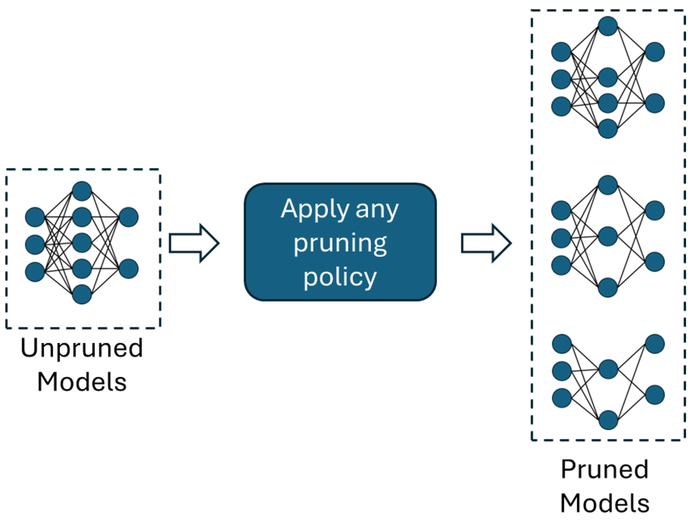
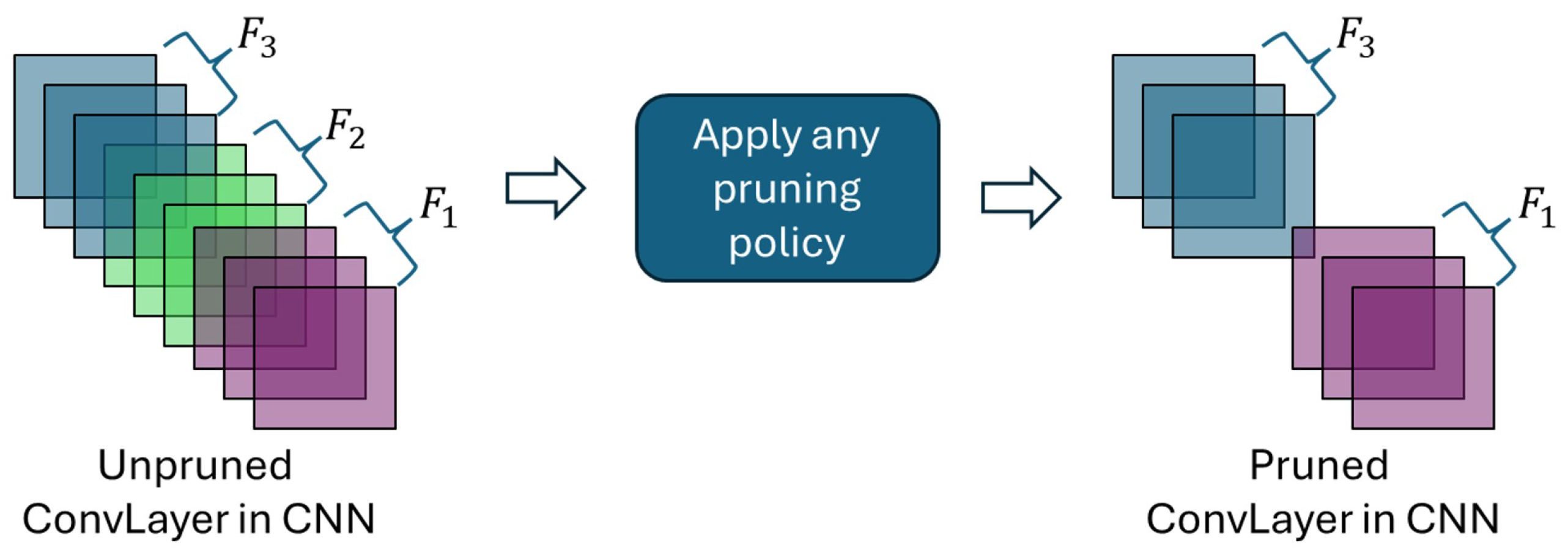
2.1. Pruning

Deep learning models have gradually increased in size over time, resulting in enhanced performance. However, an increase in parameters results in more FLOPs, making it harder to deploy these models on devices with limited resources. This results in longer inference times and increased energy consumption [30].

Several studies have shown that reducing the number of parameters in a model does not significantly impact its accuracy or overall behavior [31]. Pruning is one of the most common techniques for achieving this reduction. It involves the selective removal of connections, filters, or neurons from the network.

In the case of traditional artificial neural networks (ANNs), pruning is usually applied to a pre-trained model. This process involves defining a pruning policy that considers several factors, including the dataset, the desired pruning percentage, the pruning distribution (e.g., uniform or structured), and the criterion used to determine which elements to remove. The last component can use random strategies, neuron gradients, or magnitude-based metrics, such as the L1 or L2 norm [28].

After applying the pruning policy, the resulting model contains fewer parameters. For example, Figure 1 shows three versions of a neural network with different levels of pruning applied to the hidden layer. It illustrates how the internal structure of the model changes depending on the percentage of elements removed.

Convolutional neural networks (CNNs) are primarily composed of convolutional and fully connected layers. The fully connected layers are structurally similar to artificial neural networks (ANNs), meaning that pruning can be applied similarly. The situation is more complex in the case of convolutional layers, due to the large number of filters that operate on the input. Several strategies have been proposed to prune these layers, including element-wise, channel-wise, shape-wise, layer-wise, and filter-wise pruning [32].

The filter-wise strategy is one of the most commonly used techniques because of its simplicity and effective results. It involves removing entire filters from a convolutional layer, directly reducing computational load and memory usage. Figure 2 shows an example of filter-wise pruning. Starting from a convolutional layer with three filters, a pruning policy based on a specific criterion is applied, resulting in the removal of the filter $F_2$. This leaves a pruned version of the layer with only two active filters.

Pruning Distributions

When pruning techniques are applied to convolutional neural networks (CNNs), it is not necessary that the percentage of parameters to be removed is uniform across all layers. Different pruning distribution (PD) methods can be used to allocate the pruning ratio throughout the network, significantly impacting the model’s final performance.

Some of the most common distributions include the following (see Figure 3):

• Uniform distribution ($P{D}_1$): The same percentage of parameters is removed from each layer.
• Bottom-up ($P{D}_2$): Pruning starts lightly in the early layers and gradually increases in the deeper ones.
• Top-down ($P{D}_3$): A more aggressive pruning method is applied to the early layers and is gradually reduced in the deeper ones.
• Bottom-up/top-down ($P{D}_4$): Less pruning is applied to the first and last layers, while intermediate layers are pruned more heavily.
• Top-down/bottom-up ($P{D}_5$): More pruning is applied to the first and last layers, and less to the intermediate ones.

Although similar FLOP reductions can be achieved with different levels of parameter pruning, the impact on model accuracy can differ substantially [28].

Figure 3. Examples of pruning distributions [28].

Figure 3. Examples of pruning distributions [28].

2.2. Parameters

In both artificial neural networks (ANNs) and convolutional neural networks (CNNs), parameters are values that the model learns during training and uses to perform computations during inference. Therefore, a larger number of parameters generally results in a larger model size.

Equations (1) and (2) show how the number of parameters is calculated in a CNN, both for convolutional layers and fully connected (FC) layers [20].

$$Parameter{s}_{conv}=filters\times (W_k\times H_k\times C_k)+filters,$$

(1)

$W_o$, $H_o$ are the width and height of the output (feature map), and $filters$ are the number of filters of the current layer.

$$Parameter{s}_{F{C}^l}=(filter{s}^{l-1}\times filter{s}^l)+filter{s}^l,$$

(2)

where l is the current layer, and $l-1$ is the previous layer.

2.3. FLOPs

Floating-point operations (FLOPs) are arguably the most important metric for estimating the computational cost of performing inference on a model. This is because FLOPs are independent of the hardware used, making them a fairer basis for comparing different pruning strategies.

Equations (3)–(5) explain how FLOPs are calculated, depending on whether the operation occurs in a convolutional layer, a fully connected (FC) layer, or a pooling layer [20].

$$FLOP{s}_{conv}=2\times (W_k\times H_k\times C_k)\times (W_o\times H_o)\times filters,$$

(3)

$W_o$, $H_o$ are the width and height of the output (feature map), and $filters$ are the number of filters of the current layer.

$$FLOP{s}_{F{C}^l}=2\times (neuron{s}^{l-1}\times neuron{s}^l),$$

(4)

$neurons$ is the number of the neurons.

$$FLOP{s}_{poo{l}^l}=(W_o/S)\times (H_o/S)\times \left(filter{s}^{l-1}\right),$$

(5)

where S is the stride of the pooling operation.

2.4. Batch Size

To use an AI model, one must provide input data to analyze and process and make a decision. One of the most widely used benchmark datasets is CIFAR-10 [33], which contains images classified into ten different categories such as airplanes, dogs, horses, among others.

When feeding data into a model, this can be carried out individually or in groups. This group of inputs is known as a batch, and its size is referred to as the batch size. For example, if one image is fed into the model, the batch size is 1. If two images are fed in simultaneously, the batch size is 2, and so on.

Figure 4 illustrates how increasing the batch size directly affects the input size of the model. In the case of CIFAR-10, each image has a size of $32\times 32$ pixels with three color channels (red, green, and blue), which means that a single image has an input dimension of $3\times 32\times 32=3072$ values. If a batch size of 8 is used, the model input becomes $8\times 3\times 32\times 32$, which is eight times larger than the input for a batch size of 1.

An increase in batch size has significant implications for inference. First, it increases the number of FLOPs required. Second, it can impact the system’s inference time and energy consumption, especially when running on resource-constrained devices.

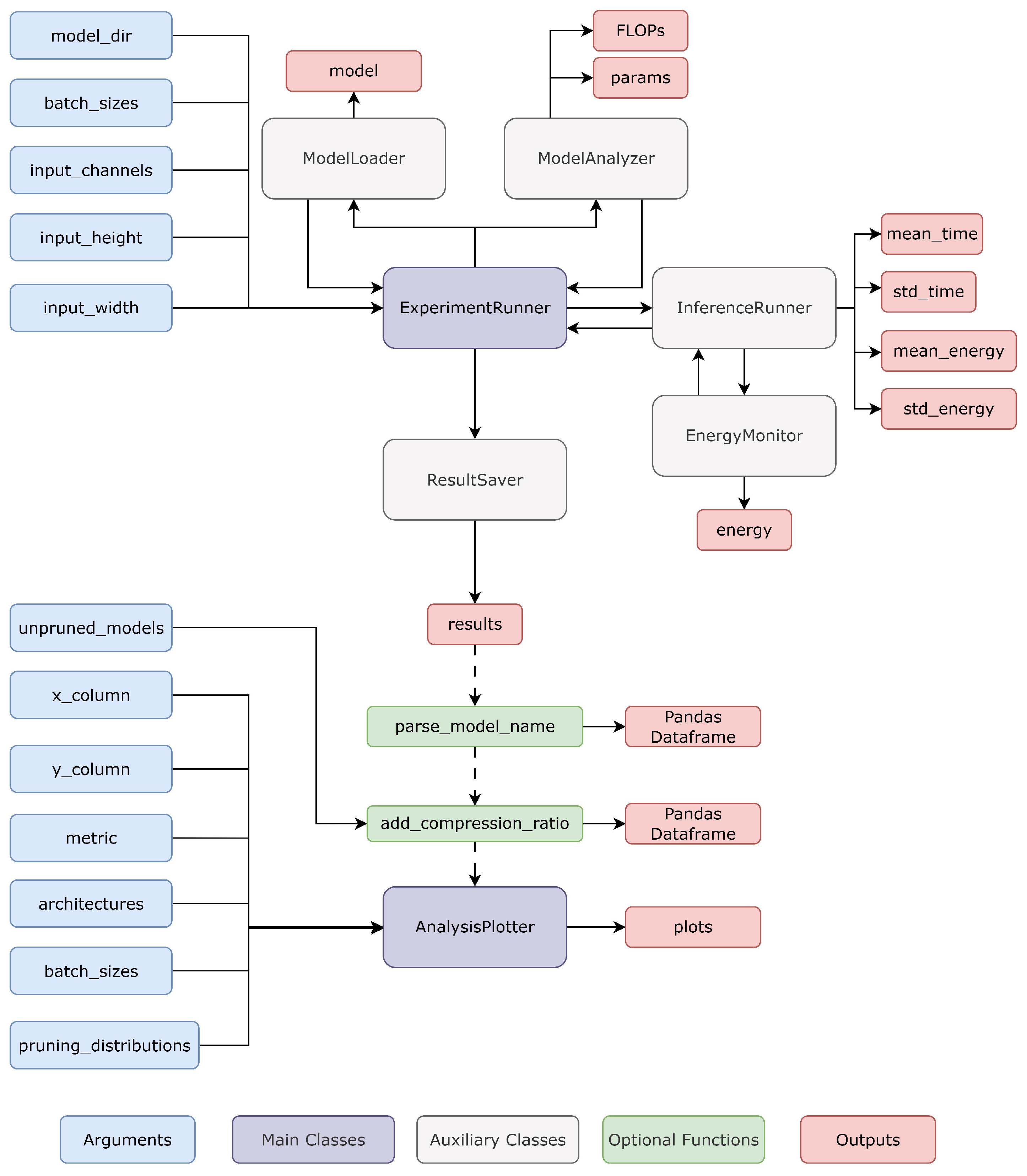
3. The Proposed PruneEnergyAnalyzer Toolkit

PruneEnergyAnalyzer is a Python-based toolkit which takes as input the unpruned model and a set of pruned models obtained by varying one or more hyperparameters: pruning method, distribution type, compression rate, or batch size. Based on these models, the tool computes the energy consumption of the unpruned model and each pruned version, and calculates the percentage of energy savings. It also computes the number of parameters and FLOPs for each model, along with their respective reduction percentages. Using these values, the tool generates comparative visualizations, as shown in the Results section. Figure 5 shows the overall workflow.

Therefore, Step 1 through Step 3 are performed outside the proposed library and are the responsibility of the user. Once the models to be compared are available, Step 4 is executed, and the comparative visualizations are obtained in Step 5.

3.1. PruneEnergyAnalyzer: Architecture

The architecture of PruneEnergyAnalyzer is organized around two main classes, a set of auxiliary modules, and some optional utilities (see Figure 6).

The core class is ExperimentRunner, which orchestrates the entire evaluation workflow: it loads pruned and unpruned models (with ModelLoader), performs parameter and FLOP analysis (with ModelAnalyzer), executes inference, monitors energy consumption workflow (with Inference Runner and ModelLoader), and stores results (with ResultSaver). It requires inputs such as the directory of the pruned models, input dimensions, and a list of batch sizes. The second main class is AnalysisPlotter, which generates comparative visualizations (e.g., energy savings vs parameter reduction) using the results provided by ExperimentRunner.

Supporting modules include the following: ModelLoader, which loads model files from disk; ModelAnalyzer, which calculates the number of parameters and FLOPs; InferenceRunner, which performs multiple inference runs to estimate execution time; EnergyMonitor, which uses NVML to measure energy consumption during inference; and ResultSaver, which compiles and saves all results into a structured format.

Additionally, there are optional utility functions such as parse_model_name, which extracts metadata (e.g., pruning method, architecture, batch size) from model names and returns a labeled DataFrame, and add_compression_ratio, which calculates parameter or FLOP-based compression ratios relative to the unpruned model.

The PruneEnergyAnalizer does not prune models; rather, it loads pruned models for analysis. To generate the results, the model names must comply with a certain nomenclature.

Pruned model names must follow a format consisting of five parameters, as follows:

$$\mathtt{ARCHITECTURE}\_\mathtt{DATASET}\_\mathtt{METHOD}\_\mathtt{PD}\_\mathtt{GPR}-\mathtt{PR}.\mathtt{pth}$$

Unpruned models follow the format

$$\mathtt{ARCHITECTURE}\_\mathtt{DATASET}\_\mathtt{UNPRUNED}.\mathtt{pth}$$

where

• ARCHITECTURE refers to the model architecture (e.g., AlexNet, VGG16);
• DATASET indicates the dataset used for training (e.g., CIFAR10);
• METHOD specifies the pruning method applied (e.g., random, LRP, SeNPIS);
• PD denotes the pruning distribution used, if applicable (e.g., PD3, PD2);
• GPR-PR indicates the pruning ratio value (e.g., 10, 20, 30);
• UNPRUNED refers to the baseline model prior to pruning.

For example, a name of the pruned model can be

$$\mathtt{VGG}\mathtt{11}\_\mathtt{CIFAR}\mathtt{10}\_\mathtt{SENPIS}\_\mathtt{PD}\mathtt{1}\_\mathtt{GPR}-\mathtt{30}.\mathtt{pth}$$

while the corresponding name of the unpruned model is

$$\mathtt{VGG}\mathtt{11}\_\mathtt{CIFAR}\mathtt{10}\_\mathtt{UNPRUNED}.\mathtt{pth}$$

In this way, if the pruned models come from different architectures, compression rates, pruning methods, distribution types, or correspond to different classification problems (datasets), the tool will automatically group them according to the different types of visualizations it generates.

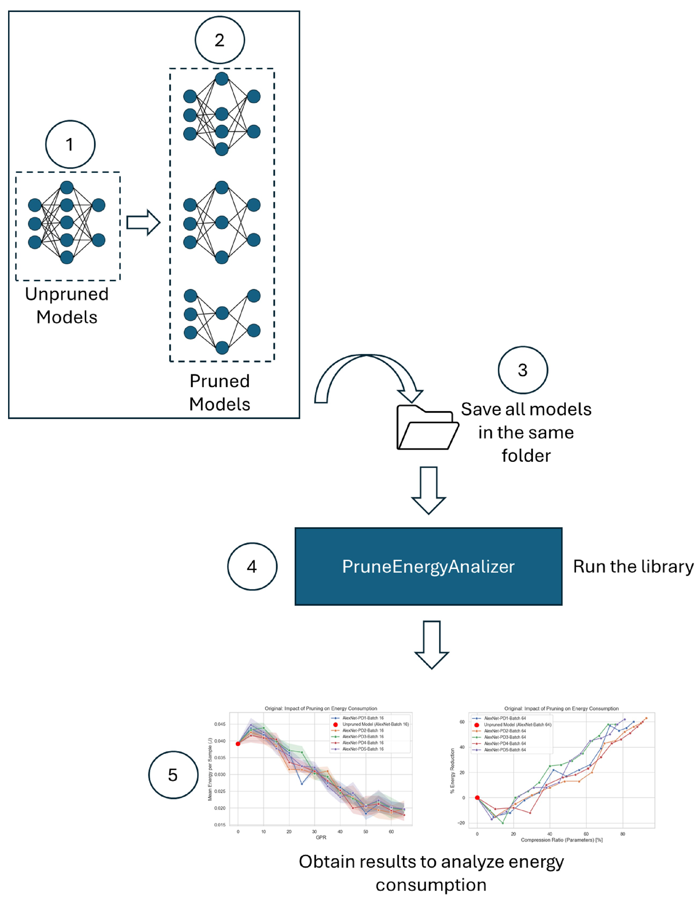
3.2. Using PruneEnergyAnalyzer

To facilitate adoption, PruneEnergyAnalyzer provides a high-level interface that simplifies experimentation and visualization workflows. The library abstracts the complexity of energy monitoring and model evaluation into modular components, enabling researchers to concentrate on analyzing results instead of implementation details. The following examples demonstrate how the toolkit can be used to evaluate the energy consumption of pruned models and generate informative visualizations.

Algorithm 1 shows the process for running energy consumption experiments on a directory of pruned models. The user must specify the path to the models (model_dir), a list of batch sizes to test. Additionally, the input shape of the data (e.g., for CIFAR-10, (3, 32, 32)) and the name of the output CSV file must be provided.

Internally, a GPU device is selected and passed to the ExperimentRunner class, which handles model loading, inference, and energy measurement. The function run_experiment() executes the full pipeline for all batch sizes and models, storing results such as Mean Energy per Sample, inference time, and model size in a DataFrame. This DataFrame is returned and also saved to disk for later analysis.

Algorithm 1: Energy evaluation of pruned models.

Once the experimentation is complete, results can be analyzed and visualized using the plotting interface, as outlined in Algorithm 2. The user must specify the name of the CSV file containing the results and the columns to use for the x- and y-axes. Optionally, a plot title can be added. Additionally, filters can be applied to restrict the visualization to specific model architectures, pruning distributions, and batch sizes.

Algorithm 2: Energy analysis and visualization.

The AnalysisPlotter class reads the CSV file and generates comparative plots across the selected configurations. These plots help reveal the relationship between compression metrics (such as parameter or FLOPs reduction) and energy consumption. This enables users to identify optimal pruning strategies based on empirical evidence.

4. Results: Illustrative Example of Use

The purpose of this section is not to determine which network or pruning distribution performs best, but rather to illustrate how an experiment can be designed to compare the energy behavior of pruned models and support decision-making beyond just FLOPs or parameter reduction.

The types of plots generated by the tool are the following:

• Impact of Compression Ratio (%) on Energy Reduction (%).
• Impact of Pruning Distribution on Energy Reduction (%).
• Impact of Network Architecture on Energy Consumption.
• Impact of Batch Size on Energy Consumption.
• Impact of Batch Size on FPS Values.

As a first step, pruned models must be generated from an original unpruned model by varying the pruning hyperparameters that PruneEnergyAnalyzer can evaluate. These include the following:

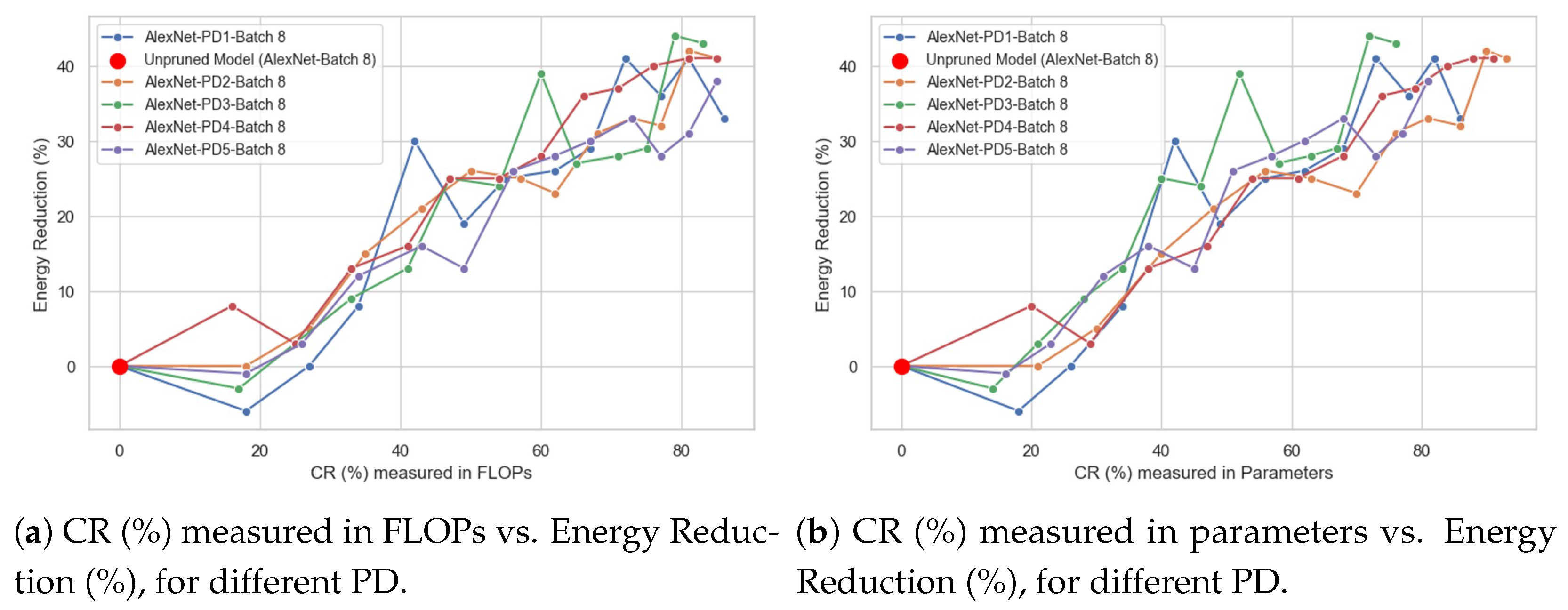
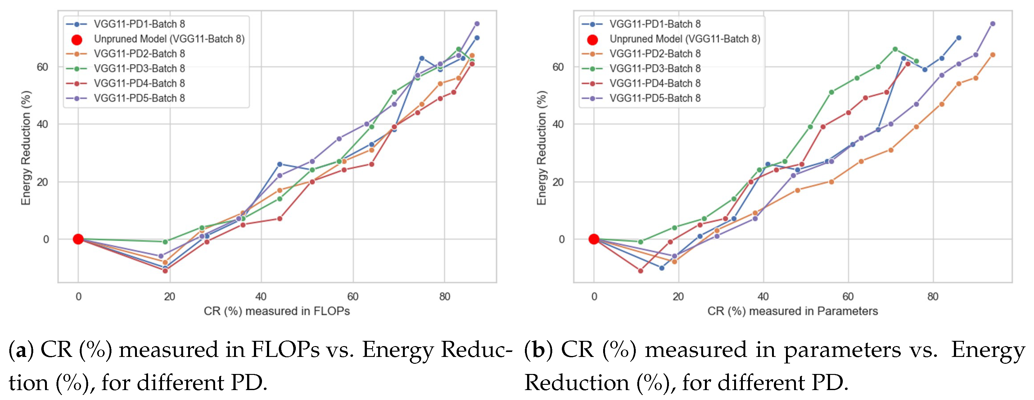
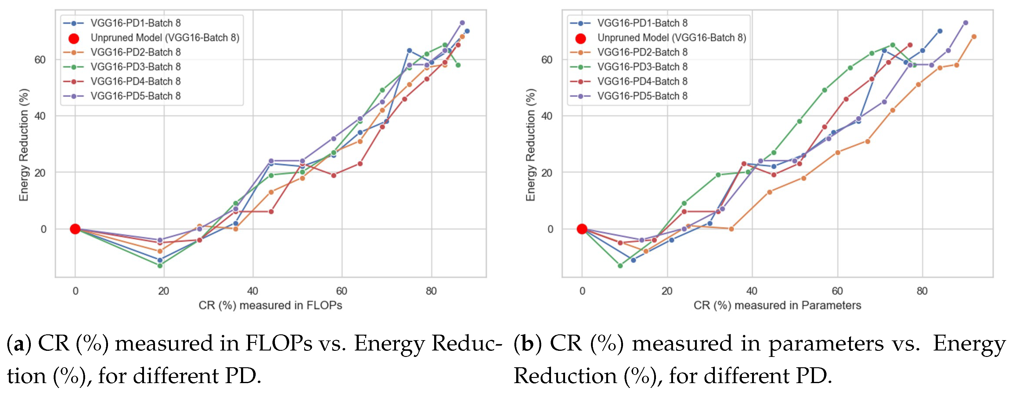
• Network architecture: We used AlexNet, VGG11, and VGG16.
• Compression ratio (CR): Twelve different CR values were selected.
• Pruning distribution (PD): Five distributions, labeled PD1 through PD5 (see Section Pruning Distributions for details).

For our experimental phase, these models were created using an external open-source tool known as FlexiPrune [34]. In total, 180 pruned models and 3 unpruned models were prepared in advance.

As a second step, models must be named following the notation

$$\mathtt{ARCHITECTURE}\_\mathtt{DATASET}\_\mathtt{METHOD}\_\mathtt{PD}\_\mathtt{GPR}-\mathtt{PR}.\mathtt{pth}$$

and then saved in the corresponding folder. In this way, by reading the model names, the tool can identify the type of plots it can generate, based on the available options from the library.

Table 1. Experimental setup for evaluating pruned models using PruneEnergyAnalyzer.

Component	Details
Hardware	NVIDIA RTX 3080 GPU
Framework	PyTorch 2.6.0+cu118
Python version	3.11
Input shape	$3\times 224\times 224$
Architectures	AlexNet, VGG11, VGG16
Pruning distributions	$P{D}_1$, $P{D}_2$, $P{D}_3$, $P{D}_4$, $P{D}_5$
Compression levels	13 (including unpruned model)
Batch sizes	1, 8, 16, 32, 64
Number of pruned models	180
Number of unpruned models	3

summarizes the experimental setup used to evaluate the pruned models with PruneEnergyAnalyzer. The experiments were conducted on an NVIDIA RTX 3080 GPU using PyTorch 2.6.0+cu118 and Python 3.11.

It is important to note that the values reported in each case correspond to the average of 10,000 trials performed for each combination of model and batch size used for the inference phase.

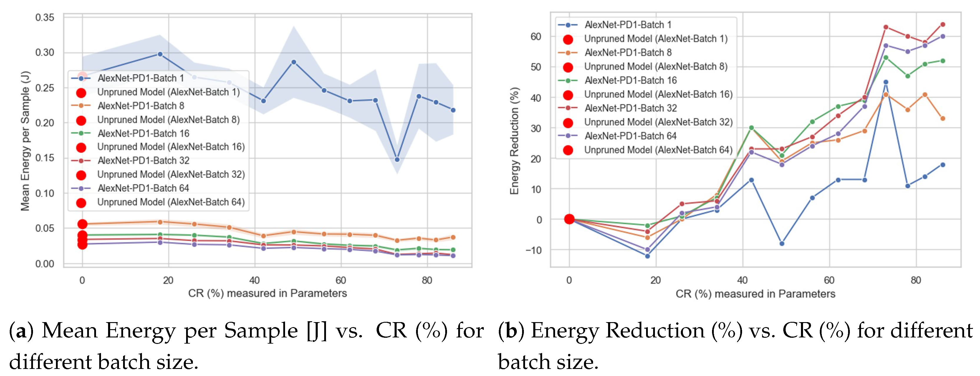
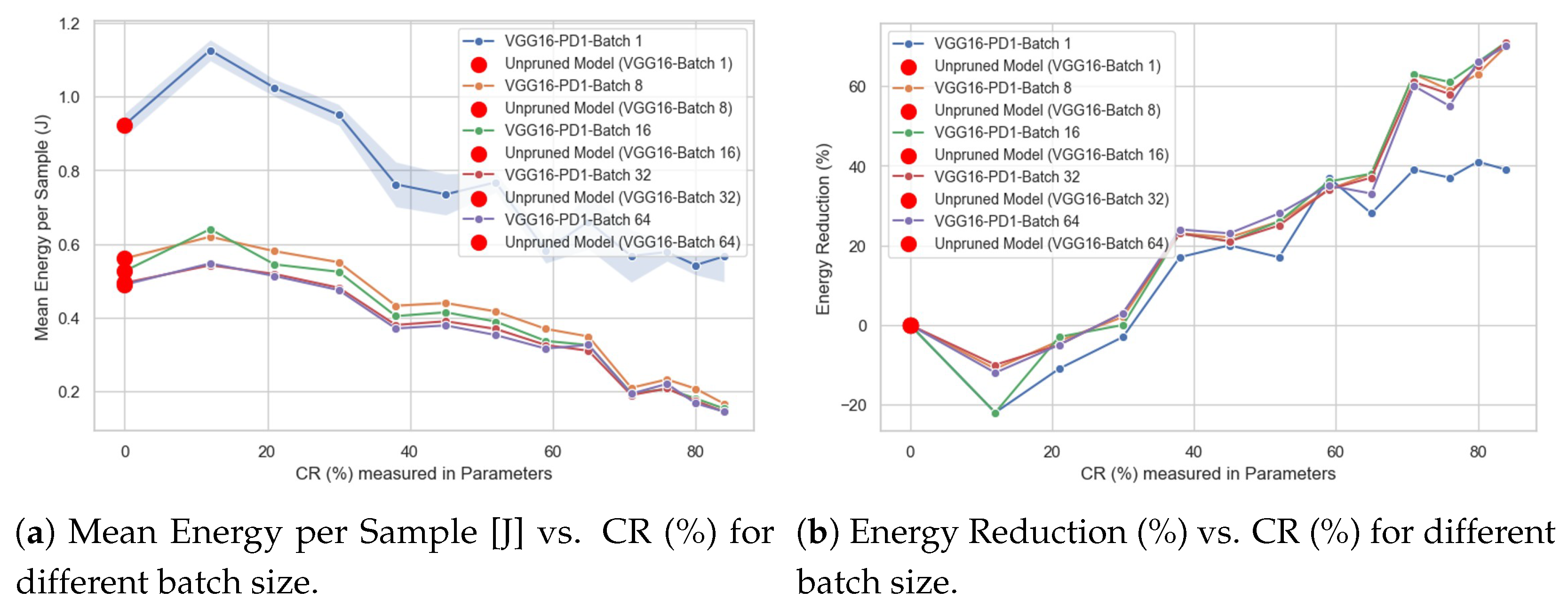
4.1. Impact of Compression Ratio (%) on Energy Reduction (%)

The purpose of generating this type of visualization is to establish a relationship between the compression ratio (CR) and the Energy Reduction, as well as to identify whether there exists a breakpoint beyond which further increases in CR no longer result in significant energy savings. To this end, PruneEnergyAnalyzer generates two types of plots:

• Compression Ratio (%) vs. Mean Energy per Sample, expressed in units of joules [J].
• Compression Ratio (%) vs. Energy Reduction (%).

The second plot is derived from the first by applying the following mathematical equation:

$$\mathrm{Energy} \mathrm{Reduction}(\%)=\left(1-{\displaystyle \frac{\mathrm{Mean} \mathrm{Energy} \mathrm{per} \mathrm{Sample} \mathrm{of} \mathrm{Pruned} \mathrm{Model}}{\mathrm{Mean} \mathrm{Energy} \mathrm{per} \mathrm{Sample} \mathrm{of} \mathrm{Unpruned} \mathrm{Model}}}\right)\times 100$$

(6)

For example, if the unpruned model has an energy consumption of 0.32 [J], and the pruned model consumes 0.1 [J], then the Energy Reduction (%) is calculated as

$$\left(1-{\displaystyle \frac{0.1}{0.32}}\right)\times 100=68.7\%$$

(7)

However, in both types of plots, the horizontal axis represents the compression ratio (%), denoted as CR (%), which is calculated as follows:

$$\mathrm{CR}(\%)=\left(1-{\displaystyle \frac{\mathrm{Size} \mathrm{of} \mathrm{Pruned} \mathrm{Model}}{\mathrm{Size} \mathrm{of} \mathrm{Unpruned} \mathrm{Model}}}\right)\times 100$$

(8)

Here, both the size of the pruned model and the unpruned model can be measured in terms of either FLOPs or the number of parameters. Therefore, the CR (%) is expressed according to one of these metrics.

For instance, if the size of the unpruned model is 120 million parameters, and the pruned model has 40 million parameters, then the compression ratio would be

$$\mathrm{CR} (\%)=\left(1-{\displaystyle \frac{40M}{120M}}\right)\times 100=(1-0.33)\times 100=66.6\%$$

(9)

indicating that the compression was measured in terms of parameters.

Figure 7 shows an example of the energy consumption for VGG11 using PD3 and a batch size of 8. Specifically, Figure 7a presents the absolute Mean Energy per Sample (in joules), while Figure 7b displays the Energy Reduction (%) relative to the unpruned model.

This type of visualization enables observations such as the following:

• The type of behavior of the CR (%) vs. Energy Reduction (%) curve, identifying whether it is linear or not. For example, one could answer the following question: does doubling the CR (%) value lead to a doubling of the Energy Reduction (%) value?
• Whether there is a “breaking point”; that is, a specific CR (%) value, measured in either FLOPs or parameters at which the direction of the curve changes. For example, in the Energy Reduction (%) curve, there could be a CR (%) value where the curve shifts from increasing to decreasing.

For example (Figure 7), the relationship between CR (%) and Energy Reduction (%) is not linear; that is, doubling CR (%) does not result in doubling Energy Reduction (%). Moreover, a breakpoint may exist around a CR (%) of 70%, beyond which further increase in CR not only fails to enhance energy savings, but actually leads to higher energy consumption, contrary to the intended effect.

4.2. Impact of Pruning Distribution on Energy Reduction (%)

In this case, the goal is to evaluate the impact of the pruning distribution (i.e., from $P{D}_1$ to $P{D}_5$) on the Energy Reduction (%) for a fixed CR(%) in terms of FLOPs or parameters. In other words, given several pruned models that achieve the same reduction but are obtained using different pruning distributions, it is desirable to determine which of them yields the greatest energy savings.

Figure 8, Figure 9 and Figure 10 present the results of the impact of the pruning distribution (PD) on energy consumption for the AlexNet, VGG11, and VGG16 networks, respectively. The plots on the left show the results when the CR (%) is measured in FLOPs, whereas those on the right correspond to CR (%) measured in terms of parameters.

This type of visualization enables observations such as the following:

• For a specific CR (%), either in terms of FLOPs or parameters, it helps determine which type of pruning distribution (PD) most effectively reduces energy consumption, and which one is the least energy-efficient.
• For a specific pruning distribution (PD), it allows identifying its energy-saving behavior as the compression rate (CR%) increases, whether in terms of FLOPs or parameters, and determining which CR(%) value is most suitable for the particular characteristics of the problem being addressed.

For example, in the case of AlexNet (Figure 8a), when the CR (%) measured in FLOPs is 60%, it is more convenient in terms of Energy Reduction to select PD3, while the least favorable option is PD2. In contrast, for both VGG11 and VGG16 (Figure 9a and Figure 10a), and at the same CR (%) value, the most suitable option is PD5, and the least recommended is PD4.

On the other hand, for both VGG11 and VGG16 (Figure 9 and Figure 10), regardless of which PD is selected, if the CR (%) measured in FLOPs or parameters is below 20%, the energy consumption will be higher than that of the unpruned model. Therefore, low CR (%) values are not recommended in terms of energy efficiency.

4.3. Impact of Network Architecture on Energy Consumption

Another aspect to consider is the relationship between Energy Reduction (%) (or Mean Energy per Sample [J]) and the type of network. It is well-known that larger networks tend to have significantly higher energy consumption compared to smaller ones. For example, VGG16 is expected to consume much more energy per sample than AlexNet. However, as the model is pruned, the resulting energy savings may lead to similar energy consumption levels between them. Therefore, it is advisable to compare these values as the CR (%) increases. This is the purpose of this type of graphs.

Figure 11 shows two graphs: the one on the left corresponds to Mean Energy per Sample [J] vs. CR (%) measured in parameters (see Figure 11a); while the one on the right shows Energy Reduction (%) vs. CR (%) measured in parameters (see Figure 11b). Both graphs refer to the AlexNet, VGG11, and VGG16 networks, with a batch size of 8.

This type of visualization enables observations such as the following:

• Compare the initial energy consumption values of the unpruned models in different architectures.
• Analyze how increasing CR (%) impacts the Mean Energy per Sample [J] or Energy Reduction (%).
• Identify which type of network meets the energy consumption requirements for a given CR (%), allowing the selection of not only the model with the lowest consumption, but also the one with the best performance (based on tests carried out outside the tool), as long as it remains below a defined threshold.

From Figure 11a, it can be observed that although the Mean Energy per Sample of VGG16 is significantly higher than that of AlexNet in their unpruned models (about 10 times greater), this difference decreases as the CR (%) increases. In other words, the Mean Energy per Sample of VGG16 approaches that of AlexNet, reaching only about four times higher at a high CR (%). This indicates that the potential for energy savings through pruning is significantly greater in larger networks. This is confirmed in Figure 11b, where the Energy Reduction (%) reaches up to 70% for both VGG11 and VGG16, far exceeding the maximum Energy Reduction (%) of AlexNet, which only reaches 35%.

Finally, if the pruned models have been evaluated using accuracy or F1 score metrics and VGG16 shows significantly better performance than AlexNet, it could be selected as long as the energy threshold is below 0.2 [J]. Alternatively, VGG11 could be chosen if the threshold is 0.1 [J] per sample.

4.4. Impact of Batch Size on Energy Consumption

Another factor that can impact energy consumption and the resulting savings in pruned models is the batch size. With the graphs generated by the tool, the user can also compare the Mean Energy per Sample for different batch size values, specifically 1, 8, 16, 32, and 64, and CR (%) while keeping the network fixed.

First, we will present the results for AlexNet (Figure 12), followed by VGG11 (Figure 13), and finally VGG16 (Figure 14). For each network, two graphs will be displayed: the first showing the curve of Mean Energy per Sample [J] vs. CR (%), and the second showing Energy Reduction (%) vs. CR (%).

This type of visualization enables observations such as the following:

• Compare the energy consumption for the same CR (%) and network across five different batch sizes (i.e., 1, 8, 16, 32, and 64).
• Analyze how energy consumption decreases for a fixed batch size as the CR (%) increases.
• Determine which batch size is most appropriate based on the energy consumption per sample requirement.

For example, based on the results shown in the previous graphs, it can be observed that as the CR (%) increases, the energy consumption per sample decreases. It is also evident that at low CR (%) values, there is a greater variation in energy consumption across different batch sizes compared to higher CR (%) values. The values obtained for batch sizes of 32 and 64 are nearly identical, indicating that it would be necessary to analyze their values of FPS (frames per second) to select the optimal option not only in terms of energy consumption but also overall efficiency.

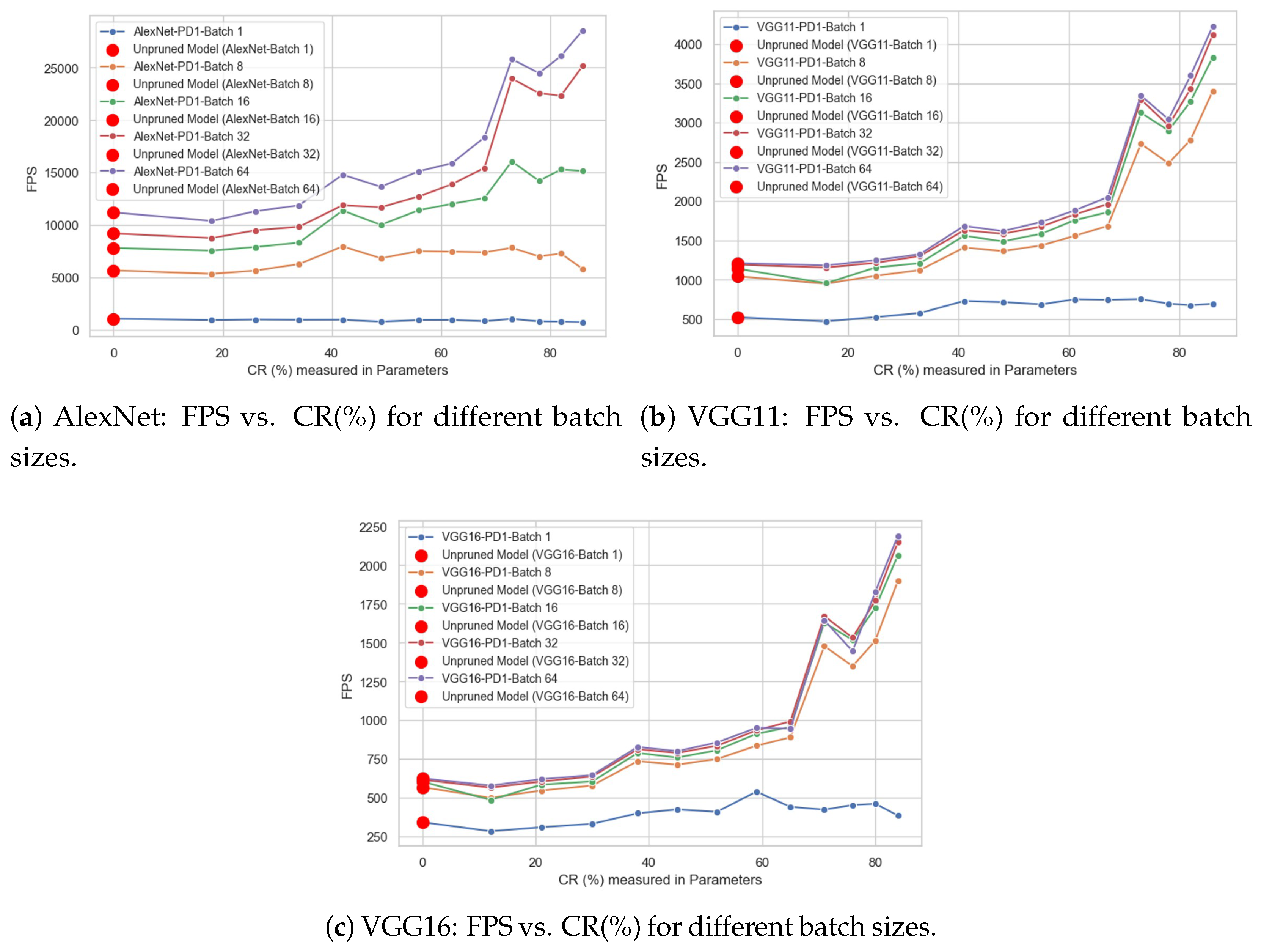
4.5. Impact of Batch Size on FPS Values

The main goal of the PruneEnergyAnalyzer library is to generate insights into energy consumption. However, its flexible visualization module, AnalysisPlotter, allows users to explore additional performance metrics by configuring different axes. For example, to study the effect of pruning on frames per second (FPS), the FPS metric can be set on the y-axis instead of energy consumption.

Figure 15 shows three graphs: the first corresponds to AlexNet (Figure 15a), the second to VGG11 (Figure 15b), and the third to VGG16 (Figure 15c). Each graph displays several CR (%) vs. FPS curves, corresponding to the five batch size values available in the tool.

This type of visualization enables observations such as the following:

• Compare FPS values for the same CR (%) and network across five different batch size values (i.e., 1, 8, 16, 32, and 64).
• Understand how FPS changes for a fixed batch size as the CR (%) increases.
• Identify which batch size is most suitable based on the FPS values.

From the previous graphs, it can be concluded that using a batch size of 1 is the worst option when aiming to achieve the highest possible FPS. The best results across all three networks and the different CR (%) values studied were obtained with a batch size of 64. As expected, AlexNet, being the network with the fewest parameters, allows the highest number of images processed per second, exceeding 25,000 for high CR (%) values. In contrast, VGG11 slightly surpasses 4000 images per second, while VGG16 remains just below 2250 images per second. To enable users to experiment with and replicate the results obtained using some of these models, thirteen of them are made available at [35].

5. Discussion

The insights presented in the previous section were derived under a specific experimental setup, including the use of a single GPU, a fixed input resolution, and a defined set of architectures and pruning distributions. Consequently, the results are not meant to be universally prescriptive. Variations in hardware, batch sizes, model architectures, or pruning strategies could lead to different energy consumption behaviors. The main objective of these experiments is not to determine a definitive optimal pruning strategy, but rather to demonstrate the capabilities and flexibility of PruneEnergyAnalyzer in generating meaningful insights regarding energy consumption across pruned deep learning models.

One such insight concerns the relationship between pruning intensity and batch size. Depending on the batch size, the results suggest that pruning too little or too much may yield negligible energy savings. For instance, in configurations with small batch sizes, pruning did not significantly reduce energy consumption, especially in lightweight architectures like AlexNet. In contrast, aggressive pruning continued to provide improvements for larger batch sizes, especially in deeper models like VGG16. These results highlight the need for case-specific pruning strategies rather than relying on general heuristics.

Another relevant observation emerged when comparing different pruning distributions. Although all distributions were designed to achieve similar overall reduction in FLOPs, their impact on energy consumption varied considerably depending on the architecture. For instance, while no single pruning distribution consistently outperformed the others in AlexNet, in the case of deeper architectures such as VGG11 and VGG16, certain distributions like $P{D}_2$ and $P{D}_4$ showed comparatively less Energy Reduction across multiple compression levels. This suggests that even when the computational cost (FLOPs) is held constant, how pruning is distributed across layers can significantly impact energy efficiency. Therefore, selecting an appropriate pruning distribution becomes critical and should be informed by experimentation rather than assumed equivalence.

An additional insight derived from the results relates to inference speed and the relationship between model compression and frames per second (FPS). While energy consumption was the primary focus, PruneEnergyAnalyzer’s flexibility enabled an analysis of performance metrics, including FPS. The experiments revealed a general trend: increasing the compression ratio improves FPS, especially when the batch size is greater than one. However, in scenarios with a batch size of one, which is often used in real-time or embedded applications, the gains in FPS from pruning were limited or even negligible, particularly in lightweight architectures like AlexNet. These results suggest that, for applications requiring single-sample inference, model compression may not offer significant performance improvements, and energy savings or latency reductions could be minimal.

Considering that excessive pruning reduces energy consumption but can negatively impact model performance particularly accuracy and F1 score, PruneEnergyAnalyzer assists users in navigating this trade-off by enabling the combination of energy data with performance metrics, such as accuracy, for each pruned model. This integration allows the generation of customized plots that reflect both energy efficiency and predictive performance.

To demonstrate this functionality, Figure 16 presents two synthetic scenario (illustrative, fabricated data). Each scenario includes two curves with their respective ranges: the blue curve represents Energy Reduction (%), while the green curve represents Accuracy Drop (%). In the first scenario, accuracy decreases very slowly, remaining nearly constant until the CR (%) reaches 60%, after which the decline becomes more pronounced. In the second scenario, accuracy drops by as much as 7%, a level that may be unacceptable in certain applications, such as clinical image classification. Now, suppose we aim to achieve the highest possible Energy Reduction with the lowest possible loss in accuracy. If the application allows a maximum accuracy drop of 3% and requires at least a 20% reduction in energy consumption, then in the first scenario, the appropriate CR range would lie between 50% and 80%, satisfying both conditions. In contrast, in the second scenario, the CR range that meets these constraints is narrower, falling between 35% and 50%. This highlights that the decision of how much to prune should not only take accuracy loss into account (even when minimal), but also consider the associated energy savings.

6. Conclusions

PruneEnergyAnalyzer is a step forward in the development of tools aligned with the principles of Green AI. Rather than relying solely on proxy indicators like parameter count or FLOPs, the toolkit enables direct measurement of energy consumption in deep learning models. This allows for more accurate, context-aware assessments of pruning strategies, fostering a shift from performance-centered design to sustainability-conscious model optimization.

Beyond its immediate functionality, PruneEnergyAnalyzer stands out for its modularity, extensibility, and ease of integration into existing workflows. It empowers researchers and engineers to evaluate energy efficiency across architectures, pruning distributions, and batch sizes while also facilitating the generation of visual insights to support decision-making. These capabilities make the toolkit particularly valuable for applications where energy is a critical constraint, such as edge computing, embedded AI, and mobile deployment.

While the toolkit does not perform pruning itself, it is compatible with any externally pruned model in PyTorch format, including models derived from widely used architectures such as ResNet or MobileNet. This flexibility enables its use in diverse experimental settings. Although the current version focuses on visualization and analysis, integrating optimization techniques (e.g., Pareto front analysis) to guide users toward optimal trade-offs between energy consumption and model performance is a promising future direction.

The illustrative examples included in the toolkit (e.g., Figure 16) are based on synthetic data and serve to demonstrate its visualization capabilities. These examples do not represent actual experimental results but aim to show how users can explore different compression-performance scenarios. Additionally, the potential integration of the toolkit with energy-efficient architectures such as Spiking Neural Networks (SNNs) offers another avenue for exploration.

By providing an open, reproducible platform for energy analysis, PruneEnergyAnalyzer encourages the community to develop and benchmark models not only for accuracy, but also for energy impact. In doing so, it contributes meaningfully to the advancement of Green AI and promotes a culture of responsible, sustainable AI development.

References

- Rawas, S. AI: The Future of Humanity. Discov. Artif. Intell. 2024, 4, 25. [Google Scholar] [CrossRef]
- Rashid, A.B.; Kausik, M.A.K. AI revolutionizing industries worldwide: A comprehensive overview of its diverse applications. Hybrid Adv. 2024, 7, 100277. [Google Scholar] [CrossRef]
- LeCun, Y.; Bengio, Y.; Hinton, G. Deep learning. Nature 2015, 521, 436–444. [Google Scholar] [CrossRef]
- Mienye, I.D.; Swart, T.G. A Comprehensive Review of Deep Learning: Architectures, Recent Advances, and Applications. Information 2024, 15, 755. [Google Scholar] [CrossRef]
- Islam, S.; Elmekki, H.; Elsebai, A.; Bentahar, J.; Drawel, N.; Rjoub, G.; Pedrycz, W. A comprehensive survey on applications of transformers for deep learning tasks. Expert Syst. Appl. 2024, 241, 122666. [Google Scholar] [CrossRef]
- Ersavas, T.; Smith, M.A.; Mattick, J.S. Novel applications of Convolutional Neural Networks in the age of Transformers. Sci. Rep. 2024, 14, 10000. [Google Scholar] [CrossRef]
- Alwakid, G.; Gouda, W.; Humayun, M.; Sama, N.U. Melanoma Detection Using Deep Learning-Based Classifications. Healthcare 2022, 10, 2481. [Google Scholar] [CrossRef]
- Bachute, M.R.; Subhedar, J.M. Autonomous Driving Architectures: Insights of Machine Learning and Deep Learning Algorithms. Mach. Learn. Appl. 2021, 6, 100164. [Google Scholar] [CrossRef]
- Lazzaroni, L.; Bellotti, F.; Berta, R. An embedded end-to-end voice assistant. Eng. Appl. Artif. Intell. 2024, 136, 108998. [Google Scholar] [CrossRef]
- Gaba, S.; Budhiraja, I.; Kumar, V.; Martha, S.; Khurmi, J.; Singh, A.; Singh, K.K.; Askar, S.S.; Abouhawwash, M. A Systematic Analysis of Enhancing Cyber Security Using Deep Learning for Cyber Physical Systems. IEEE Access 2024, 12, 6017–6035. [Google Scholar] [CrossRef]
- Wermelinger, M. Using GitHub Copilot to Solve Simple Programming Problems. In Proceedings of the 54th ACM Technical Symposium on Computer Science Education V. 1, New York, NY, USA, 15–18 March 2023; SIGCSE 2023. pp. 172–178. [Google Scholar] [CrossRef]
- PyTorch Team. Deep Learning Energy Measurement and Optimization | PyTorch. 2025. Available online: https://pytorch.org/blog/zeus/ (accessed on 6 February 2025).
- Hamilton, J. Data Center and Cloud Innovation. Keynote at CIDR 2024. 2024. Available online: https://mvdirona.com/jrh/talksandpapers/JamesHamiltonCIDR2024.pdf (accessed on 27 July 2025).
- Alizadeh, N.; Castor, F. Green AI: A Preliminary Empirical Study on Energy Consumption in DL Models Across Different Runtime Infrastructures. In Proceedings of the IEEE/ACM 3rd International Conference on AI Engineering–Software Engineering for AI, New York, NY, USA, 14–15 April 2024; CAIN ’24. pp. 134–139. [Google Scholar] [CrossRef]
- Martinez, M. The Impact of Hyperparameters on Large Language Model Inference Performance: An Evaluation of vLLM and HuggingFace Pipelines. arXiv 2024, arXiv:2408.01050. [Google Scholar]
- Qi, Q.; Lu, Y.; Li, J.; Wang, J.; Sun, H.; Liao, J. Learning Low Resource Consumption CNN Through Pruning and Quantization. IEEE Trans. Emerg. Top. Comput. 2022, 10, 886–903. [Google Scholar] [CrossRef]
- Li, J.; Louri, A. AdaPrune: An Accelerator-Aware Pruning Technique for Sustainable CNN Accelerators. IEEE Trans. Sustain. Comput. 2022, 7, 47–60. [Google Scholar] [CrossRef]
- Just, F.; Ghinami, C.; Zbinden, J.; Ortiz-Catalan, M. Deployment of Machine Learning Algorithms on Resource-Constrained Hardware Platforms for Prosthetics. IEEE Access 2024, 12, 40439–40449. [Google Scholar] [CrossRef]
- Park, S.; Kim, H.; Kim, H.; Choi, J. Pruning with Scaled Policy Constraints for Light-Weight Reinforcement Learning. IEEE Access 2024, 12, 36055–36065. [Google Scholar] [CrossRef]
- Pachón, C.G.; Ballesteros, D.M.; Renza, D. SeNPIS: Sequential Network Pruning by class-wise Importance Score. Appl. Soft Comput. 2022, 129, 109558. [Google Scholar] [CrossRef]
- Rajaraman, S.; Siegelman, J.; Alderson, P.O.; Folio, L.S.; Folio, L.R.; Antani, S.K. Iteratively Pruned Deep Learning Ensembles for COVID-19 Detection in Chest X-Rays. IEEE Access 2020, 8, 115041–115050. [Google Scholar] [CrossRef]
- Fontana, F.; Lanzino, R.; Marini, M.R.; Avola, D.; Cinque, L.; Scarcello, F.; Foresti, G.L. Distilled Gradual Pruning with Pruned Fine-Tuning. IEEE Trans. Artif. Intell. 2024, 5, 4269–4279. [Google Scholar] [CrossRef]
- Yang, T.J.; Chen, Y.H.; Emer, J.; Sze, V. A method to estimate the energy consumption of deep neural networks. In Proceedings of the 2017 51st Asilomar Conference on Signals, Systems, and Computers, Pacific Grove, CA, USA, 29 October 2017–1 November 2017; pp. 1916–1920. [Google Scholar] [CrossRef]
- Yang, T.J.; Chen, Y.H.; Sze, V. Designing Energy-Efficient Convolutional Neural Networks Using Energy-Aware Pruning. In Proceedings of the IEEE Conference on Computer Vision and Pattern Recognition (CVPR), Honolulu, HI, USA, 21–26 July 2017. [Google Scholar]
- Kinnas, M.; Violos, J.; Kompatsiaris, I.; Papadopoulos, S. Reducing inference energy consumption using dual complementary CNNs. Future Gener. Comput. Syst. 2025, 165, 107606. [Google Scholar] [CrossRef]
- Huang, D.; Xiong, Y.; Xing, Z.; Zhang, Q. Implementation of energy-efficient convolutional neural networks based on kernel-pruned silicon photonics. Opt. Express 2023, 31, 25865–25880. [Google Scholar] [CrossRef]
- Zhang, Q.; Zhang, R.; Sun, J.; Liu, Y. How Sparse Can We Prune A Deep Network: A Fundamental Limit Viewpoint. arXiv 2023, arXiv:2306.05857. [Google Scholar]
- Pachon, C.G.; Pinzon-Arenas, J.O.; Ballesteros, D. Pruning Policy for Image Classification Problems Based on Deep Learning. Informatics 2024, 11, 67. [Google Scholar] [CrossRef]
- Beckers, J.; Van Erp, B.; Zhao, Z.; Kondrashov, K.; De Vries, B. Principled Pruning of Bayesian Neural Networks Through Variational Free Energy Minimization. IEEE Open J. Signal Process. 2024, 5, 195–203. [Google Scholar] [CrossRef]
- Brown, T.; Mann, B.; Ryder, N.; Subbiah, M.; Kaplan, J.D.; Dhariwal, P.; Neelakantan, A.; Shyam, P.; Sastry, G.; Askell, A.; et al. Language Models are Few-Shot Learners. Adv. Neural Inf. Process. 2020, 33, 1877–1901. [Google Scholar]
- Goel, A.; Tung, C.; Lu, Y.H.; Thiruvathukal, G.K. A Survey of Methods for Low-Power Deep Learning and Computer Vision. In Proceedings of the 2020 IEEE 6th World Forum on Internet of Things (WF-IoT), New Orleans, LA, USA, 2–16 June 2020; pp. 1–6. [Google Scholar] [CrossRef]
- Liang, T.; Glossner, J.; Wang, L.; Shi, S.; Zhang, X. Pruning and quantization for deep neural network acceleration: A survey. Neurocomputing 2021, 461, 370–403. [Google Scholar] [CrossRef]
- Krizhevsky, A. Learning Multiple Layers of Features from Tiny Images; Technical Report; University of Toronto: Toronto, ON, Canada, 2009. [Google Scholar]
- Pachon, C.G.; Pinzon-Arenas, J.O.; Ballesteros, D. FlexiPrune: A Pytorch tool for flexible CNN pruning policy selection. SoftwareX 2024, 27, 101858. [Google Scholar] [CrossRef]
- Pachon Suescun, C.G.; Ballesteros L, D.M.; Pedraza, C. PruneEnergyAnalizer. 2025. Available online: https://data.mendeley.com/datasets/cc2cd723hb/1 (accessed on 27 July 2025).