Enhanced Face Recognition in Crowded Environments with 2D/3D Features and Parallel Hybrid CNN-RNN Architecture with Stacked Auto-Encoder

Abstract

Face recognition (FR) in unconstrained conditions remains an open research topic and an ongoing challenge. The facial images exhibit diverse expressions, occlusions, variations in illumination, and heterogeneous backgrounds. This work aims to produce an accurate and robust system for enhanced Security and Surveillance. A parallel hybrid deep learning model for feature extraction and classification is proposed. An ensemble of three parallel extraction layer models learns the best representative features using CNN and RNN. 2D LBP and 3D Mesh LBP are computed on face images to extract image features as input to two RNNs. A stacked autoencoder (SAE) merged the feature vectors extracted from the three CNN-RNN parallel layers. We tested the designed 2D/3D CNN-RNN framework on four standard datasets. We achieved an accuracy of $98.9\%$. The hybrid deep learning model significantly improves FR against similar state-of-the-art methods. The proposed model was also tested on an unconstrained conditions human crowd dataset, and the results were very promising with an accuracy of $95\%$. Furthermore, our model shows an 11.5% improvement over similar hybrid CNN-RNN architectures, proving its robustness in complex environments where the face can undergo different transformations.

1. Introduction

In many applications, including mobile intelligent visual human-computer interfaces, smart surveillance, and law enforcement, FR in crowded environments is crucial [1]. However, FR is still challenging in uncontrolled settings. The look of the face, including changes in position, changes in illumination, facial expressions, and occlusions, is one of the issues presented by these situations [2,3]. One of the most difficult problems in pattern recognition across various areas is identifying individual faces in images or movies that contain many faces. However, there are still far fewer facial recognition systems available for developers in research and development of applications that may use this technology. Research has focused on developing efficient Deep Learning (DL) models for FR and on robust facial feature extraction. While robust facial feature extraction seeks to extract strong face representations, deep learning methods typically increase classification and recognition accuracy. Examples of texture-based information that complements 2D elements include skin tone, facial features, and curves. With this knowledge, modifications to posture, lighting, and facial expressions might be more reliable. Nevertheless, 3D features are invariant to pose and light changes since they offer geometric depth and shape information. 3D features allow accurate facial structure modeling whatever any environment.

Studies on face detection and recognition have produced positive results on specific data sets in recent years. Several researchers decided to use much simpler techniques to noisy and crowded real-world data. In many real-world applications, such as auto-login systems, emotion identification, and access control, the obtained results are unsatisfactory. The suggested approach seeks to identify faces in natural settings. The designed approach proposed in this study enhances face recognition in noisy and unconstrained data. It employs vanishing and regularization loss in conjunction with a regularization technique. The development of extremely reliable applications and studies in contemporary face recognition research is supported by deep learning techniques. The approach has been successfully tested on datasets, but in noisy and congested datasets that are typically used in real-world applications, the results are not as satisfactory as one would hope. The main goal of this work is to go in-depth into facial recognition studies in noisy and crowded environments. The effectiveness of an FR system is mainly due to the feature extraction and classification phases [4]. 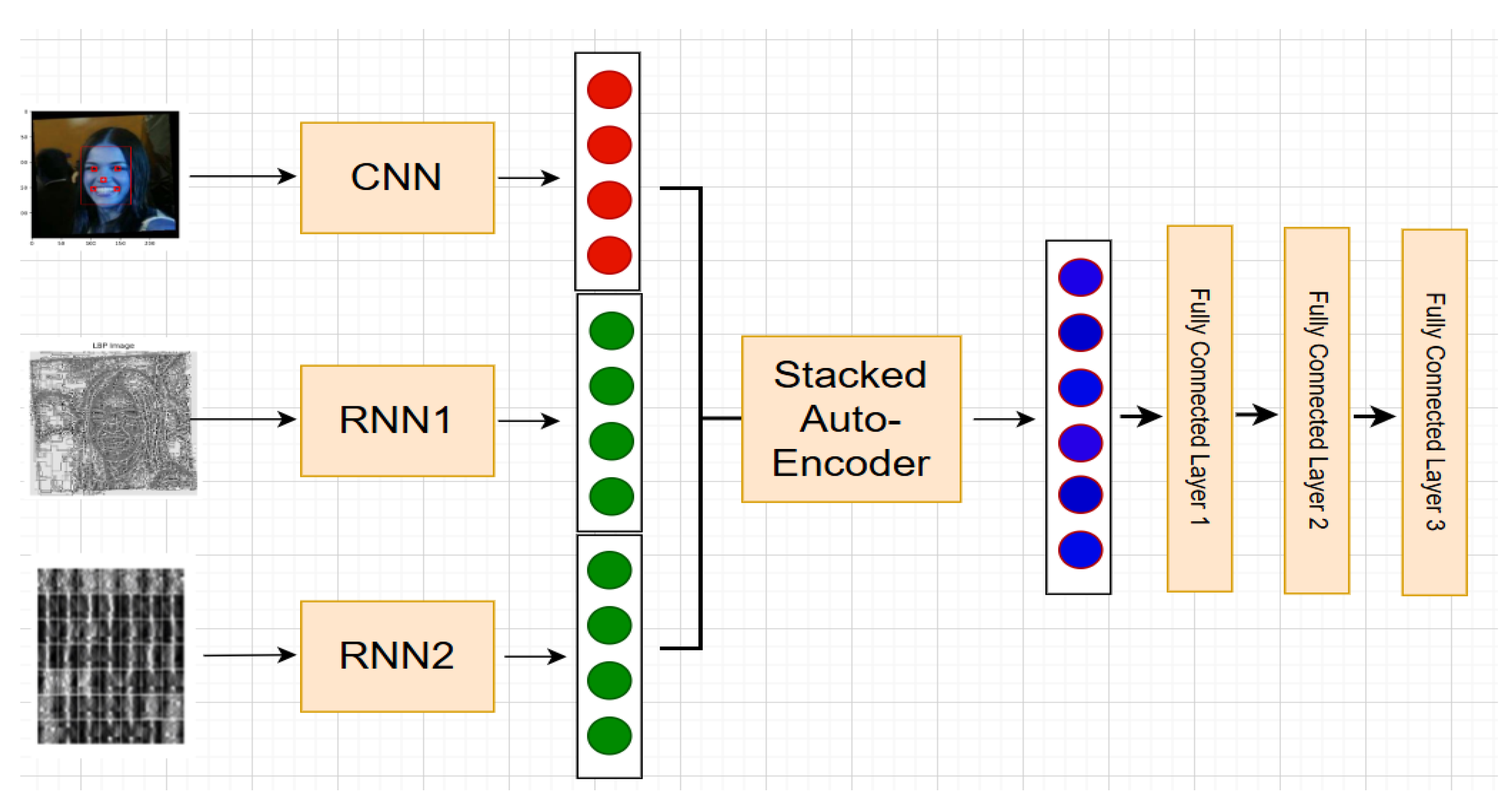Our goal in this paper is to recognize faces under various transformations using robust facial feature extraction based on facial color, texture, and shape [5]. Convolutional neural networks (CNN) and recurrent neural networks (RNN) are used in combination in the proposed method. FR is regarded as a sequence classification problem. Using CNN and RNN feature extraction layers operating in parallel, our designed architecture for FR begins by creating features from three inputs. The semantic and non-redundant characteristics were then retrieved using the SAE. Proposing three fully connected layers for ultimate decision-making was the last phase. This paper summarizes its main contributions as follows:

• To achieve invariance against changes in illumination, position, and emotions, we extract 2D features [6] and 3D features [1,7] from the extracted face. The main contribution of this work is the selection and combination of 2D and 3D descriptors. This enables the production of a powerful facial description despite potential changes in congested and real-world scenarios. Our developed architecture uses three inputs: the face image, the 3D mesh LBP image, and the LBP image.
• We used the generated 2D/3D features based on color, texture, and shape as input to generate three parallel hybrid CNN and RNN networks to extract the best facial features. Each input offers distinct and complementary data. We can extract complementing features that are specific to each modality’s capabilities by customizing CNN and RNN for each input. The computational efficiency and portability of parallel hybrid CNNs and RNNs make them perfect for real-time applications or processing enormous datasets. To get the most information out of their particular input type, each CNN and RNN may focus on design optimization.
• The retrieved features are combined using an SAE to provide the optimal representation of a global feature vector that will be the input for two fully connected layers for FR. The feature vectors obtained by CNNs and RNNs can have less dimensions thanks to an SAE. By doing this, we eliminate unnecessary data and retain only the most significant and practical information.
• A softmax decision function was presented to recognize the face after three fully connected layers. Using four distinct datasets, the developed framework was assessed and compared with comparable state-of-the-art models. In uncontrolled circumstances, the CNN-RNN model’s parallel multimodal architecture improves FR accuracy.

This is how the remainder of the paper is structured. We provide a quick overview of the related works in Section 2. We describe our designed FR approach in unconstrained environments in Section 3. The experimental evaluation is reported in Section 4. The paper is concluded and some suggestions for future work are presented in Section 5.

2. Related Works

The process of automatically recognizing or identifying a person from a single image or set of images is known as facial recognition (FR). Three modules are needed for the automated FR system [8]. First, a face detector finds faces in images or videos. Using a face landmark detector to align the faces to standardize canonical coordinates is the second step. Third, we design the FR module using these aligned face images. According to the authors in [9], FR algorithms are made up of the connection between feature extraction and categorization. In a crowded environment, the facial image can be impacted by changes in size, occlusion, motion blurring, viewpoint, illumination, and expression. In real-time face recognition, visibility variance from a variety of potential ambient variables presents a major challenge. Determining how different facial attributes contribute to recognizing a person’s identity is one of the main issues in FR. These challenges are now an important factor limiting FR’s effectiveness in crowded environments [10]. Changes in skin tone, texture, and illumination can be well detected with 2D facial features. Changes in face position, changing viewpoints, occlusion, and geometric variations of the face can all be detected with 3D facial features.

An approach for FR based on deep learning and 2D feature extraction was proposed by the authors in [11]. In the literature, numerous 3D FR techniques have been put out [12]. To decrease posture fluctuation, several works have employed 3D techniques as a transitional step. Furthermore, under some circumstances that are challenging for 2D systems to handle, Geometric information can also be included in 3D face data, which may improve recognition accuracy [13]. Authors in [14] proposed a 3D morphable face model of Gaussian mixture (GM-3DMM). The entire population is represented as a collection of Gaussian subpopulations, each with a mean and a common covariance. These models employ 3D facial data from Caucasian, Chinese, and African individuals. The problem of 3D-assisted 2D FR when the input image is subject to degradation or shows intrapersonal fluctuations that the 3D model is unable to capture has been addressed by the authors in [15]. They acquire knowledge of a subspace bounded by modifications resulting from image deterioration and missing modes of variation. Instead of using 3D capture, they employ reconstructed 3D facial data from 2D photos. The research’ findings showed that this strategy results in extremely competitive FR performance. The authors in [16] used features that were taken from various features based on local covariance operators.

In recent years, deep learning has been successfully applied in a number of computer vision domains, particularly for FR [17]. On the LFW dataset, proposed deep learning-based methods have overcome the challenges in uncontrolled environments and obtained recognition accuracy of over 99% [18]. Bahroun et al. presented a Deep 3D-LBP network [1]. Using shape and texture data, the proposed method creates a face feature image that is then fed as input into the neural network for training. In light of this work, another approach was proposed in [19]. The challenge is to reconstruct 3D facial information from 2D images. For FR, they then combined form and texture local binary patterns (LBP) on a mesh using the Mesh-LBP technique. Lastly, they used a deep autoencoder to generate a small data representation based on the face image descriptors they acquired from the Mesh-LBP. The authors in [20] present HResAlex-Net, a unique deep learning model for 2D and 3D facial recognition. The proposed model consists of a mixed Convolutional Neural Network (CNN) structure designed to recognize faces by integrating several biometric data types.

Deep learning approaches still have several limitations, even if they have produced remarkable results in FR. One of the primary disadvantages of deep learning models is their computational expense. Moreover, these models might be susceptible to variations in noise, pose, and illumination. Another drawback of deep learning is the challenge of identifying the learned features. The discriminative properties of the top layers in CNN designs are known to be greater than those of the lower layers. Face recognition commonly uses the features of the fully connected (FC) layers. Two concerns could be pointed out in this regard: first, is FC feature efficiency superior to others? Second, is it possible to integrate FC features to make them work better together?

To the best of our knowledge, the several earlier works on FR that are now available address Question 1. This study aims to provide an answer to Question 2. For multimodal face biometrics, the authors of [21] proposed multi-feature fusion layers, which led to dual-stream convolutional neural networks learning significant and illuminating data. Specifically, this network uses two progressive components with various fusing algorithms to collect RGB data and texture descriptors for multimodal facial biometrics. In [22], the authors demonstrated that complex situations greatly impair the recognition performance of a single DCNN. For facial recognition and verification, they propose a multi-feature DCNN ensemble learning method based on machine learning. They used a number of existing network models, such as ResNet50 and SENet, to enhance and integrate functionality.

CNNs are frequently used in image classification, while recurrent neural networks (RNNs) are rarely used. The main use of CNNs is to analyse visual data, including images and movies. They are quite good at identifying patterns and spatial hierarchies. RNNs are efficient to process time series data or natural language, where temporal dynamics or order are crucial. Some researchers tried to deal with the image classification problem accurately by combining CNNs and RNNs. The most popular approach involves using a CNN to extract spatial image features, which are then fed into an RNN [23]. To classify the images, the authors in [24] employed CNN and RNN to extract features. They then concatenated the features from the two different deep networks using a straightforward early fusion. In order to classify Alzheimer’s disease in medical image processing, CNN and RNN were first combined in [25]. In [26], a parallel structure divides biopsy images into four classes. A CNN and an RNN make up the suggested architecture for extracting image features. The features extracted by the two distinct neural network structures of the model were then combined using a unique perceptron attention mechanism that was developed from the natural language processing (NLP) sector. In [27], the challenge of classifying plant species based on images of their leaves is addressed. Combining the ResNet50 and IFRVFLC models, the authors proposed a hybrid ResNet50 with an intuitionistic fuzzy RVFL classifier (IFRVFLC) model. The ResNet50 model first employs the leaf image textures to acquire the deep features, and then it applies principal component analysis as a feature reduction technique to retrieve the important features. To classify leaf images, the PCA features are extracted and fed into the IFRVFLC architecture. In [28], the author proposed a novel multimodal 2D/3D BiLSTM-CNN parallel architecture for face recognition in unconstrained conditions. In order to enhance recognition performance against different variations that the face might experience in real-world scenarios, the proposed parallel CNN architecture comprises three subnetworks for feature extraction that can fully exploit the 2D/3D features extracted from the face: the Local Binary Pattern image (LBP), 3D mesh-LBP, and the face image itself. To extract the most important information from the feature vectors generated by parallel CNNs, a BiLSTM model is proposed, followed by two fully connected layers for the FR.

To maximize the information provided by 2D and 3D features, we propose a new design for FR that combines both of these data types. Because CNNs can recognize patterns like edges, textures, and facial landmarks, they are excellent at extracting spatial data from face images. It is possible to simulate the order in which the extracted 2D and 3D facial features depend on each other using RNNs. In dynamic identification scenarios, they can identify patterns in both space and time, such as variations in the face’s depth or between frames. The RNN adds global temporal and relational characteristics from the 2D and 3D inputs to the CNN’s localized spatial features. The CNN and RNN feature vectors are compressed into a lower-dimensional latent space by the SAE. This process preserves important information while lowering the computational cost for later phases (like classification). It successfully blends complementary data from the temporal RNN and spatial CNN domains. To strengthen the final representation, SAEs can function as denoising autoencoders, removing unnecessary information or noise from the feature vectors. This enhances its capacity to generalize to unobserved facial images, particularly in unregulated settings. By concentrating on important features and disregarding noise or extraneous details, the autoencoder’s compression and reconstruction process helps minimize overfitting.

3. Designed Deep CNN-RNN Architecture for Face Recognition

The recognized face images may change resolution, pose, and illumination when FR is applied to images or videos in crowded environments. Consequently, several standard preprocessing methods, like image resampling and normalization, need to be used. Many features can be extracted from these face images. The color feature is extracted from the full-face image. Furthermore, we extract texture and shape features by matching 2D images with a generic 3D face model. First, we use the Dlib operator to locate landmarks and perform facial detection [29]. Second, we propose to extract 2D/3D texture, shape, and color information from the detected face in order to get descriptors with the most accurate and significant representation of the face. The texture descriptor is capable of handling changes in illumination. Using form descriptors, emotions can be effectively identified. The color descriptor provides information on the colors of skin and hair. To do this, we model the texture map difference between the reference images and the 3D aligned input images. At the same time, we learn 2D color and texture features using the Local Binary Pattern for Color Images (LBPC) [6] and extract face features using the mesh-LBP [7]. A single face image or face description cannot encompass all of the identifying information. Therefore, FR cannot be performed in busy areas using the conventional single-input CNN design. In this study, we developed a novel multi-modal CNN architecture that uses multi-processing to accept three images as input concurrently.

The generated face descriptors are then fed into a multi-input CNN-RNN architecture that has been developed. We describe every step of the suggested approach for FR in full below. The challenge of creating a “good and efficient” deep architecture is still unresolved [30]. The suggested multi-modal CNN-RNN architecture is explained in this section. Even though deep CNNs have demonstrated remarkable performance in facial recognition tasks, non-deep CNN architectures can still get good results. In some cases, such as when working with tiny datasets or when computational resources are restricted and the recognition response is binary, the incorporation of image characteristics like LBPC pictures or Mesh-LBP can be helpful [31,32]. When a face in different images have variations in pose, lighting, emotions, or occlusion, the characteristics that are retrieved from these three inputs are combined to form a powerful face feature that is not much affected. To achieve the greatest facial recognition, we want our multi-processing CNN method to exploit all of this information simultaneously during the classification phase. The designed architecture of the parallel multi-input CNN for parallel face identification is shown in Figure 1.

The input from the first fully connected layer is the output of the SAE. Additionally, we use the triplet loss function to train our model [17]. The triplet loss approach compares three images at once: an anchor, a positive (an image of the same class), and a negative (an image of a different class). It causes the anchor to become more isolated from the negative and less isolated from the positive.

Additionally, the Adam optimizer is used for optimization [33]. We employ 128 sample mini-batches. We apply dropout at a rate of $0.25$ before the two fully linked layers to regularize the model. We trained our CNN for 500 epochs with a starting learning rate of $0.001$. The learning rate is adjusted over epochs. This is called learning rate scheduling and is a key technique to improve training stability and model performance. In our case, for each 50 epochs, we reduce the learning rate by a fixed factor (0.1). By preventing overfitting, dropout forces the network to rely more on dispersed representations and less on individual neurons. By producing slightly different iterations of the model with each iteration, dropout also increases the robustness of the model; it aids the network in learning a variety of representations.

3.1. The CNN Module

We use a tiny neural network to extract features from the face image. In the learning phase, the network gets better at identifying and categorizing face images. Two convolutional layers (C), a max-pooling layer (M), and a locally connected layer (L) for feature extraction make up our proposed CNN architecture. The main difference between a convolutional layer and a locally connected layer is that the filter in a convolutional layer is shared by all the pixels in a facial image. On the other hand, in the locally connected layer, each neuron (pixel) has its own filter. This type of layer allows the network to learn various types of features for different parts of the face. This has been useful to many researchers, particularly for face verification jobs [34]. For example, the areas between the eyes and the eyebrows have a far larger capability for differentiation and a distinct appearance than the areas between the lips and the nose. When local layers are used, the computational effort of feature extraction remains the same, but the number of parameters that need to be trained changes [35]. This could lead to an increase in the number of parameters in our network since the number of parameters will be multiplied by the number of output neurons. A tiny CNN design like ours could help us avoid these kinds of problems. The first convolutional layer (C1) has 32 filters and measures $11\times 11$. These 32 feature maps, one for each channel, are sent to a $3\times 3$ max-pooling layer (M1) with stride of 2. A second convolutional layer (C2) with 16 filters of size $9\times 9$ comes next. The following layer (L1) is locally linked and consists of 16 filters. Only the most pertinent aspects are extracted by tiny CNNs, which ignore extraneous information and concentrate on important face landmarks like the mouth, nose, and eyes. Smaller CNNs are more computationally efficient and appropriate for real-time applications since they have fewer layers and parameters.

Let I $\in {\mathbb{R}}^{H\times W\times C}$ be the input face image. The CNN is defined over L layers. For the l-th layer, we have:

$$X^{\left(l\right)}=\sigma \left(W^{\left(l\right)}\ast X^{(l-1)}+b^{\left(l\right)}\right),l=1,\dots ,L$$

(1)

$$X^{\left(0\right)}=I$$

(2)

the final CNN feature vector is obtained by flattening the output of the last convolutional layer.

$$f_{\mathrm{CNN}}=\mathrm{flatten}\left(X^{\left(L\right)}\right)$$

(3)

CNN parameters are:

$${\theta }_{\mathrm{CNN}}=\{W^{\left(l\right)},b^{\left(l\right)}\mid l=1,\dots ,L\}$$

(4)

3.2. The RNN1 Module

The 2D Local Binary Pattern (LBP) descriptor [36] creates binary patterns by comparing the intensity of each pixel with its circular neighborhood in order to represent facial texture. To capture microstructures like edges and spots, these patterns are combined into histograms over local regions (such as a grid of rectangular blocks). LBP is frequently used for face recognition since it is computationally efficient and resistant to monotonic lighting variations. While multi-scale LBP improves discriminative capability, variations such as uniform LBP minimize dimensionality by grouping patterns. The descriptor is generated in the form of an image feature with the same size as the original image and is a fundamental component of texture-based facial analysis due to its ease of use and efficiency. An image has spatial properties. A time-sequence relationship exists between the image’s pixels at the pixel level. RNNs may process images by treating image patches or pixel rows/columns as sequences. A legitimate method for modeling spatial relationships as temporal sequences in RNNs used for image feature extraction is to treat the image height as time steps and the width as feature dimensions. This is an explanation of how this operates and what it means: The RNN treats each row of pixels (height dimension H) as a time step. The input characteristics at that time step are the pixels in a row (width dimension W). The RNN processes H steps, each with W features, for a [H, W] grayscale image. There are frequently structural relationships between adjacent rows (e.g., edges, textures). Like a time series, the RNN’s hidden state “remembers” features from earlier rows [26].

Applying an RNN to a face’s LBP image might be a useful method for capturing spatial correlations between various facial areas as well as local texture patterns from the LBP. The LBP approach captures fine-grained texture information, and an RNN can be used to illustrate the connections between these patterns in various facial regions. The idea behind using an RNN for an LBP image is to treat various facial regions as successive “tokens” or “steps”. These stages will then be processed by the RNN, which will record the dependencies between the patterns in different regions. The LBP image is divided into many (16 × 16) non-overlapping sections. Sliding or overlapping windows may be able to capture more fine features, but they increase the RNN memory problems sequence. To separate features such as each eye, the upper and lower lips, the bridge and tip of the nose, and occasionally finer elements like the eyelids and brows separately, we have selected 16*16 non-overlapping zones. Anatomical dependencies in faces are directed. There are spatial-semantic links between facial features, including the mouth, nose, and eyes. For this purpose, the RNNs model ordered progression more accurately than CNNs or transformers.

We follow a systematic pipeline that transforms spatial texture information into sequential data to use Local Binary Pattern (LBP) histograms calculated from non-overlapping image grids as input to an RNN. We calculate a histogram of the LBP values for every region (grid), which can be used as a feature vector for that area. The texture patterns within each region are compactly represented by the histogram. There are 59 bins in each area histogram. There are 58 distinct rotation-invariant patterns in uniform LBP, plus one bin for non-uniform patterns. The RNN uses each histogram as a timestep input. We arrange the areas’ feature vectors sequentially. After that, an RNN receives this sequence. To extract the time sequence features of the pixels, we employed a two-layer stacking LSTM as the RNN module [37]. Performance may be impacted by the sequence in which regions are fed into the RNN. We select rows (top to bottom, left to right across each row). The sequence length is the number of grids per image in the RNN input layer structure, which is equal to $64,59$. All of the retrieved faces are being resized to $128\times 128$ pixels. Eight-by-eight grids make up each image. The RNN will learn patterns and relationships across the texture regions of the face by processing each grid independently and sequentially. Each histogram is processed by the Bi-LSTM layers. Both left-to-right and right-to-left dependencies are captured. The left eyebrow histogram, for instance, represents timestep 1. The right eyebrow histogram is timestep 2. Use the RNN’s final hidden state as input to a fully connected layer for face recognition and then a softmax layer for classification. The Chin histogram is timestep 64. Contextual dependencies are accumulated by hidden states.

We assume the LBP image is processed as a sequence of feature vectors ${\left\{x_t^{2\mathrm{D}}\right\}}_{t=1}^T$. The RNN1 computes:

$$h_t^{2\mathrm{D}}=\sigma \left(W_x^{2\mathrm{D}}{x}_t^{2\mathrm{D}}+W_h^{2\mathrm{D}}{h}_{t-1}^{2\mathrm{D}}+b^{2\mathrm{D}}\right),t=1,\dots ,T^{2\mathrm{D}}$$

(5)

with an initial state $h_0^{2\mathrm{D}}=0$ (or learned). The final 2D feature is:

$$f^{2\mathrm{D}}=h_T^{2\mathrm{D}}$$

(6)

the parameters for this RNN1 are:

$${\theta }^{2\mathrm{D}}=\{W_x^{2\mathrm{D}},W_h^{2\mathrm{D}},b^{2\mathrm{D}}\}$$

(7)

this approach creates a powerful representation for a range of facial analysis tasks by utilizing both spatial dependencies across the face and local texture information. It accomplishes this by fusing the sequence modeling of RNN with the texture sensitivity of LBP. Fine-grained details are captured by LBP, whereas interdependence between facial areas can be modeled using RNN. Different expressions can be indicated by subtle variations in texture patterns across different facial regions. Furthermore, age frequently causes changes in texture patterns, and distinct texture shifts indicate particular emotions. To describe spatial-textural dependencies in faces, RNNs efficiently transform LBP histograms of image grids into a series of fixed-length vectors. This method uses recurrence to model region interactions while maintaining spatial locality through grids.

3.3. The RNN2 Module

The geometric features taken from 3D face models are obtained using the 3D mesh-LBP descriptor [1]. The 2D detected face is converted into 3D using the surry face model [14]. The steps that follow will be used to determine the mesh-LBP. First, the plane created by the inner-corner landmark points of the two eyes and the tip of the nose is calculated. We selected these three landmarks because they are the most reliable indicators of facial expressions and may be detected with the highest accuracy. Using simple geometric computation, we derive from these landmarks an ordered and regularly spaced set of points on that plane. After rotating the plane by a predetermined amount to better match it with the face orientation, we project this set of points onto the face surface along the plane’s normal direction. The outcome of this method is an ordered grid of points that defines an atlas for the facial areas that will divide the facial surface. The 7 × 7 constellation is made up of 49 points on the grid. We extract a neighborhood of features around each grid point after the grid of points has been defined. Each neighborhood can be defined by the set of facets that make up a geodesic disk or a sphere with a grid point at its center. 91 × 91 pixels make up the 3D Mesh-LBP face descriptor image [1]. The image feature can be conceptualized as a 7 × 7 constellation made out of a grid. For each constellation, we then produce a flattened 1D feature vector. The input of the RNN will be a sequence of all 49 feature vectors. After that, an RNN receives this sequence. The stacked LSTM with two layers was used as the RNN module to extract the time sequence features of the pixels [37]. Similarly, let the 3D Mesh-LBP be represented as a sequence

$${\left\{x_t^{3\mathrm{D}}\right\}}_{t=1}^{T^{3\mathrm{D}}}.$$

the RNN2 is defined as:

$$h_t^{3\mathrm{D}}=\sigma \left(W_x^{3\mathrm{D}}{x}_t^{3\mathrm{D}}+W_h^{3\mathrm{D}}{h}_{t-1}^{3\mathrm{D}}+b^{3\mathrm{D}}\right),t=1,\dots ,T^{3\mathrm{D}}$$

(8)

with $h_0^{3\mathrm{D}}=0$ (or a learned initial state), and the final 3D feature is:

$$f^{3\mathrm{D}}=h_T^{3\mathrm{D}}$$

(9)

the parameters for this RNN2 are:

$${\theta }^{3\mathrm{D}}=\{W_x^{3\mathrm{D}},W_h^{3\mathrm{D}},b^{3\mathrm{D}}\}$$

(10)

for face recognition, we use the final hidden state of the RNN as input to a fully connected layer, followed by a softmax layer for classification.

3.4. The Stacked Auto-Encoder Module

The architecture should be designed to extract the most valuable components of the CNN and RNN features together while reducing the amount of redundant ones and employing a stacked autoencoder for feature fusion. We demonstrate the possible structure of the stacked autoencoder architecture. We applied an early fusion to the three feature vectors extracted from the CNN and the two RNNs. After that, we decided to employ three levels of encoding. In the first level we maintain 80% of the original input dimension. Once the initial dimensionality reduction is achieved, this layer begins capturing the relationships and interactions between features extracted from both the CNN and the two RNNs. This layer preserves the most original elements while eliminating negligible alterations. Without sacrificing any useful features, the initial compression makes sure that noise and unnecessary information are filtered. With a dense layer of units $50\%$ of the preceding layer, Layer 2 further reduces. ReLU is the activation function. This layer preserves crucial spatial-temporal patterns while balancing feature reduction and capturing more abstract interactions. At this point, dimensionality reduction helps concentrate on the most useful regions of the feature space while optimizing storage and computational expenses. The last layer of the encoder, referred to as the latent space or bottleneck layer, Layer 3, minimizes redundancy while capturing the most important information from the CNN and RNN outputs. The bottleneck layer is a dense layer with even fewer units (20% of the input dimension). The feature vector is compressed into a low-dimensional, highly informative representation in this last layer. To maintain the essential information for subsequent tasks like classification or clustering, this stage makes sure the final representation is computationally efficient. The activation function is also ReLU.

To train the auto-encoder, an asymmetric decoder frequently reconstructs the bottleneck layer’s input. This guarantees that the encoder will learn to effectively and meaningfully compress the input. By minimizing reconstruction error, we train the auto-encoder. Usually, mean squared error (MSE) is used as the loss function. As a result, the encoder is forced to eliminate unnecessary information and prioritize important features. After training, only keep the encoder portion and trash the decoder. After training, we use the encoder’s output (bottleneck layer output) as the input to the fully connected layers in our main model. The concatenated feature vector: $F=[f_1;f_2;f_3]\in {\mathbb{R}}^D$ where D is the sum of sizes obtained from the three feature vectors. F represents the combined raw feature set from all three models.

A stacked autoencoder is made up of several layers of autoencoders, each of which has been taught to compress and rebuild its input while maintaining crucial information. Let L be the SAE’s buried layer count. A compressed representation is learned by each layer. The First Hidden Layer is represented by this equation:

$$h^{\left(1\right)}=\sigma \left(W^{\left(1\right)}F+b^{\left(1\right)}\right)$$

(11)

where:

• $W^{\left(1\right)}\in {\mathbb{R}}^{h_1\times D}$ is the weight matrix,
• $b^{\left(1\right)}\in {\mathbb{R}}^{h_1}$ is the bias vector,
• $\sigma \left(x\right)$ is the activation function,
• $h^{\left(1\right)}\in {\mathbb{R}}^{h_1}$ is the first hidden layer representation.

For subsequent hidden layers: l ($(2\le l\le L)$:

$$h^{\left(l\right)}=\sigma \left(W^{\left(l\right)}{h}^{(l-1)}+b^{\left(l\right)}\right)$$

(12)

where $h\left(l\right)\in \mathbb{R}hl$ is the compressed feature at layer l.

In the final layer L, we obtain the representation of the fused features:

$$z=h\left(L\right)\in \mathbb{R}hL$$

(13)

which serves as the compact yet information-preserving feature vector. For the decoder stage, it attempts to reconstruct the original feature vector:

$$\widehat{y}=\sigma (W^{\prime \left(1\right)}{h}^{\left(1\right)}+b^{\prime \left(1\right)})$$

(14)

where $W^{\prime \left(1\right)}\in {\mathbb{R}}^{D\times h_1}$, and the reconstruction error is minimized using Mean Squared Error (MSE):

$$L={\parallel F-\widehat{F}\parallel }^2$$

(15)

after training, we discard the decoder and use only the encoded representation z:

$$z=h\left(L\right)$$

(16)

this final fused feature vector preserves all information from the three input features while removing redundancy.

The selection of reduction ratios entails striking a balance between progressive compression (progressively enforcing compact representations), dimensionality reduction (removing noise and redundancy), and information retention (avoiding excessive loss of discriminative characteristics). The reduction ratios of 80%, 50%, and 20% for the three encoding layers of the Stacked Auto-Encoder (SAE) in a feature fusion process were chosen based on empirical best practices in deep representation learning and dimensionality reduction, as well as theoretical concepts. The theoretical foundations are as follows:

• Information Bottleneck (IB) theory: deep networks learn by compressing input data while maintaining pertinent information for the task, according to the IB principle [38]. When irrelevant noise like redundant CNN activations or RNN hidden states is removed through progressive compression, which involves layers reducing dimensionality one by one, only task-relevant features are kept. These include important spatial-temporal patterns.
• Manifold hypothesis: High-dimensional data (e.g., CNN+2 RNN concatenated features) lie on a lower-dimensional manifold. A gradual reduction ($80\%\to 50\%\to 20\%$) helps the SAE discover this manifold structure without collapsing too aggressively.
• Deep Learning Optimization: a more aggressive compression early (e.g., $50\%$ in the first layer) risks losing useful features prematurely. A slower compression (e.g., $90\%$ at each step) retains redundancy, defeating the purpose of SAE.

Experimentally, to justify the compression ratios ($80\%,50\%,20\%$) for a 3-level SAE, we must compute the Mean Square Error (MSE) for train/test for each level at different bottleneck sizes. Also, we need to analyze the trade-off between compression and reconstruction quality and show hierarchical error propagation across levels. The

Table 1. Stacked Autoencoder MSE Analysis Vs Compression Ratio (CR).

Level	CR	Train MSE	Test MSE	Diff MSE (Test-Train)
1	80%	0.0017	0.0019	+0.0002
1	50%	0.0036	0.0042	+0.0006
1	20%	0.0086	0.0095	+0.0009
2	80%	0.0032	0.0037	+0.0005
2	50%	0.0059	0.0066	+0.0007
2	20%	0.0150	0.0164	+0.0014
3	80%	0.0058	0.0065	+0.0007
3	50%	0.0123	0.0135	+0.0012
3	20%	0.0226	0.0260	+0.0034

is a complete table-based justification.

Empirical data from MSE on both training and test sets supports the choice of compression ratios ($80\%,50\%$, and $20\%$) across the three levels of a stacked autoencoder (SAE) as a trade-off between reconstruction quality and dimensionality reduction. Table 1 shows that at level 1, the difference between the train and test MSE is $+0.0002$, indicating a small but manageable loss. The recreation is of almost flawless quality. For this level, a ratio of $90\%$ will yield a train MSE of $+0.00015$, which is computationally wasteful but a tiny improvement. The difference between the train and test MSE for level 2 and a 50% compression ratio is $+0.0007$, which is extremely near to the difference for an $80\%$ ratio. The compression and information retention are well-balanced here. For level 3, a $20\%$ compression ratio maintains latent structure but has a poor rebuilding rate. Because they maintain important information at every level, the compression ratios of $80\%,50\%$, and $20\%$ are ideal. According to MSE, they maximize compression while minimizing reconstruction loss.

4. Experimental Results

We start by outlining the hardware specifications in this section. We then go over the datasets that were used during the experiment. Next, we test the propose approach for FR against a number of challenges including as position, lighting, and changes in facial expressions. An ablation study and the explainability of the CNN-RNN architecture for face recognition are presented at the end of this section.

4.1. Hardware Details

We are using Jupyter Notebook 7.4.2 to run Python code on a Windows computer. Our goal was to make use of our local system’s 8–10 core parallelism. Nevertheless, we chose to cease running the Google Colaboratory code because of time restrictions and the project’s remaining burden. Because the local machine may run the same code with 8–10 cores, whereas Colab only has 2 cores available, this has an impact on the results. Because it enables the execution of more instructions in parallel, multicore is advantageous for parallel applications. The findings did not demonstrate the anticipated performance boost because we only employed two cores. However, when the model is operating in parallel, we can observe notable improvements in outcomes when we take resource restrictions into account. Compared to serial programming, parallel programming has a two-fold shorter execution time. We detect and align images of faces with the 68 points surrounding the face using the Dlib operator for data preparation [29]. All recognized face photos were preprocessed by normalizing them to $128\times 128\times 3$. The models were trained over 50 epochs using ArcFace 3P2S as the loss function [39]. Every experiment was carried out using Python 3.9.13 and Keras 3.9.2 on an i9 computer. Keras mixed precision training was utilized to train the models used in this study [40].

We present in

Table 2. Specifications and training metrics for hybrid model on the LFW dataset.

Component	CNN	RNN1	RNN2	SAE + FC
Input shape	128 × 128 × 3	16 × 59	16 × 59	(512→256→128) + 3 FC
Trainable parameters	1 M	1.2 M	0.9 M	0.8 M
Training time per epoch	38 s	29 s	27 s	20 s
Ram usage (GB)	9	6	5	3
Batch size	64	128	128	256
Inference speed (FPS)	62	118	132	210
Latency per frame (ms)	16.1	8.5	7.6	4.8
CPU utilization (%)	12	9	8	6

a structured specifications and training metrics for a Parallel CNN + Two RNN architecture for face recognition, where feature vectors are fused via a Stacked Autoencoder (SAE) and classified using three fully connected (FC) layers.

Table 2 shows that, as a result of convolutions, the CNN parallel branch is the slowest (38 s/epoch) yet has the highest accuracy. The RNNs suffer from some emotion confusion, although they are faster (28 s/epoch). Because of its massive filters, CNN takes up most of the VRAM (9 GB). Larger batches are made possible by the RNNs’ low weight (5–6 GB). Only 3 GB of overhead is added by the SAE fusion. With little information loss, the SAE reduces 512-D features (CNN+RNNs) to 128-D. The discriminative properties, which help to better discriminate emotions, are further refined by the FC layers. Because of convolutional operations, the CNN has the highest latency ($16.1$ ms). Although the RNNs increase sequential dependency, they are faster (7–9 ms). The inference speed for the end-to-end system is 48 FPS, which satisfies “real-time” standards (>30 FPS) at the expense of batch processing. For live video, the latency frame per second is $20.8$ ms, which is acceptable (less than 50 ms is indiscernible to humans).

4.2. Used Datasets and Evaluation Metrics

We used four datasets to evaluate our proposed CNN-RNN architecture which are as follows:

• The LFW dataset [18]: Labeled Faces in the Wild (LFW) was developed and is regularly updated by researchers at the University of Massachusetts. The $\mathrm{13,233}$ images of 5749 people collected on the internet were recognized and centered using the Viola-Jones face detector. Photos belonging to 1680 individuals in the collection have two or more distinct images.
• The YTF dataset [41]: It was collected from 3425 YouTube videos representing 1595 individuals, a subset of the celebrities in the LFW. These videos are divided into 5000 video pairs and 10 splits in order to evaluate video-level face verification.
• The CMU Multi-PIE face dataset [42]: It includes more than $\mathrm{750,000}$ worth of images of 337 people shot in up to four sessions over five months. The subjects were photographed in 19 various lighting conditions and from 15 different perspectives, displaying a range of facial expressions.
• The Bosphorus dataset [43]: It includes 4666 images of 105 persons in different poses, action units, and occlusion conditions. Neutral and expressive scans (the six fundamental expressions (disgust, anger, fear, happiness, sorrow, and surprise) as well as scans with Action Units, rotations, and occlusions) are represented by a number of dataset subsets.

For the evaluation protocol, we used these metrics:

1.

Accuracy: The degree to which the true value and the predicted value fit is indicated by the recognition accuracy, which is important for assessing the model’s capacity for learning. In relation to all of the test’s predictions, it indicates the overall number of accurate predictions that were returned inside the FR. The accurracy is computed as follows:

$$Accuracy={\displaystyle \frac{TP+TN}{TP+TN+FP+FN}}$$

(17)

where $TP$, $TN$, $FP$, and $FN$ represent true positives, true negatives, false positives, and false negatives, respectively. We also compute precision, recall, and F1-score, which are computed as follows:

$$Precision={\displaystyle \frac{TP}{TP+FP}}$$

(18)

$$Recall={\displaystyle \frac{TP}{TP+FN}}$$

(19)

$$F1\text{-}score=2\times {\displaystyle \frac{Precision\times Recall}{Precision+Recall}}$$

(20)

2.

Roc curve: A predictive model’s true positive rate (TPR) against false positive rate (FPR) trade-off can be illustrated by the Receiver Operating Characteristics (ROC) curve. Stated otherwise, it indicates the model’s capacity to differentiate a particular class based on the expected probability. Plotting the TPR on the y-axis against the FPR on the x-axis is known as a ROC curve.

Cross-validation was used in this study to ensure that the validation accuracy results are trustworthy and applicable to other comparable circumstances. The dataset is split into K folds or pieces using this method. We choose K = 5. In this way, we split our datset to 80% training and 20% validation per fold. This is a balanced trade-off between computational cost and reliable evaluation. After that, the model is trained and validated 30 times, with the remaining folds serving as the training set and a different fold serving as the validation set each time. To provide a more accurate assessment of the model’s performance, the validation data are averaged.

4.3. Face Recognition Under Pose and Illumination Changes

In this test, we compare our method with several recent and comparable state-of-the-art techniques. The comparison focuses on the identification rate under varying illumination and pose angles.

Table 3. Accuracy (%) on various poses under neutral illumination on the Multi-PIE [42] and the YTF datasets [41].

Type	Method	−45°	−30°	−15°	+15°	+30°	+45°
2D	Liping et al. [44]	86.4	92.5	93.6	93.7	90.9	85.7
2D	Al-Aboodi et al. [45]	91.4	93.8	94.1	94.2	93.1	87.3
2D	SF-VF+LBP [46]	88.5	91.4	97.2	97.8	94.8	89.1
3D	Hejing et al. [47]	93.2	95.9	96.8	97.1	95.3.	91.7
3D	Mallikarjun et al. [15]	97.6	95.7	96.3	97.7	95.3	92.8
3D	Bahroun et al. [1]	96.3	98.2	96.1	98.4	97.9	94.4
2D + 3D	Proposed method	96.9	98.8	99.4	99.5	98.6	96.9

provides a summary of the general findings.

Based on the features used, we separate the compared approaches into two classes: 2D and 3D methods. The suggested multimodal 2D/3D CNN-RNN architecture performs better than any deep design that uses 2D and 3D features separately according to the results shown in Table 3. In general, the findings indicate that most 3D techniques can achieve higher accuracy rates than 2D techniques, particularly when there is a significant amount of pose variation ($\pm {45}^{\circ }$). This advantage comes from the 3D model’s ability to reduce the posture effect. Nonetheless, the suggested approach performs better than the 2D and 3D approaches. This is because our approach allows us to comprehend different positions. Table 3 shows that 2D features are susceptible to drastic changes in pose (profile views). It may result in a significant misalignment of characteristics. Sensor noise often affects 3D features, which record depth and geometric shape but lack texture. Large position changes and various angles of view don’t affect 3D facial features. Even in situations with severe angles or partial occlusions, their depth information aids in face recognition. We improve face identification by combining 2D and 3D data, utilizing the advantages of both approaches, particularly when there are significant posture changes. Accurate geometric features that are independent of position changes are provided by 3D data. In partial occlusions, 2D deep learning models can supplement missing data. However, both 2D texture and 3D shape become unreliable when a significant section of the face is covered by hands, hair, masks, or scarves. Motion blur, occlusions, noisy depth data, and missing 3D inputs can all cause the method to fail. To improve performance, future systems should incorporate multi-view analysis, real-time stabilization, and deep learning-based fusion. Hybrid 2D + 3D pose-invariance systems are more effective at pose-invariant face recognition for real-world applications such as driver monitoring, AR/VR, and face recognition; nevertheless, they require adjustments to operate with fewer sensors and process in real time.

4.4. Facial Expression Invariant Face Recognition

Emotion detection is a challenging task because facial expressions can be affected by pose variations, lighting, occlusions, and individual differences. The proposed multimodal 2D/3D method has been tested on the Bosphorus dataset, which presents seven variations in facial expressions. The comparative results are shown in

Table 4. Validation accuracy (%) against different facial expressions using the Bosphorus dataset [43].

Method	Neutral	Anger	Disgust	Fear	Happy	Sad	Surprise
Atik et al. [48]	98.68	78.87	81.16	80	97.17	95.45	95.77
Naim et al. [49]	100	95.77	88.41	81.41	88.68	96.97	92.96
Deng et al. [16]	100	97.2	94.2	97.1	96.2	98.5	98.6
Liang et al. [50]	100	94.37	85.51	97.14	69.23	98.59	98.52
Bahroun et al. [1]	100	97.18	93.11	100	97.47	98.88	100
Proposed method	100	97.34	96.75	100	97.63	98.96	100

.

In terms of performance, the proposed approach performs better than the most advanced and similar state-of-the-art methods. Moreover, the maximum accuracy is consistently obtained with neutral emotions. Additionally, a number of methods attain an accuracy of $100\%$, as the most common emotion is a neutral expression. However, its accuracy decreases with changing facial expressions because fear, sadness, and happy are frequently the most difficult emotions to predict.

We can conclude from Table 4 that our proposed approach works better than the most advanced techniques, particularly when the feeling is not neutral. The utilization of texture and shape elements is what gives this edge. By utilizing the advantages of both modalities, combining 2D and 3D characteristics improves emotion identification. Some important facial features, like the lips and eyes, may become partially or completely obscured when the face is twisted. The geometric structure of the face is captured using 3D depth maps, which enables the inference of expressions even in non-frontal stances. Wrinkles, variations in skin tone, and microexpressions are examples of texture and appearance-based cues that are captured by 2D features. Micro-expressions are quick, tiny facial movements that convey emotions that are otherwise hidden. While 3D features capture little muscle deformations that reveal micro-expressions, 2D captures subtle texture changes. Even with these benefits, 2D/3D techniques may still be ineffective in some situations. These techniques may not be able to extract enough emotion-related information in real-world situations or when there are severe face occlusions. 3D characteristics may not match 2D textures accurately if a person is posing in an extremely exaggerated manner (e.g., tilting their head sideways). Some emotions involve blended expressions (sad-smiling), making it difficult to classify them correctly. Hybrid 2D + 3D emotion detection systems are more accurate and reliable for real-world uses, like AI assistants, security monitoring, and healthcare. However, they need to be carefully optimized for sensor limitations and differences in the real world.

To highlight the effectiveness of the proposed method in face emotion recognition, we show the confusion matrix of 7-class facial expression recognition. The results are reported in

Table 5. Validation accuracy (%) across facial expressions using the Bosphorus dataset [43].

Method	Neutral	Anger	Disgust	Fear	Happy	Sad	Surprise
Neutral	99.4	0	0	0	0	0.4	0.2
Happy	0.5	98.7	0.2	0.3	0	0.3	0
Disgusted	0	1.1	95.4	1.4	1.2	0	0.9
Fear	0	1.3	0	97.6	0	0	1.1
Surprise	0	1.1	0	0	98.1	0	0.8
Angry	2.1	0	0	0	0	96.9	0.9
Sad	1.4	0	0	0	0	0.5	98.1

.

The results shown in Table 5 demonstrate that misclassifications are reflected by the off-diagonal values. Fear, Sad, and Surprise are frequently mistaken for one another ($0.8\%$ misclassified as Sad, $0.8\%$ as Surprise). Perhaps because neutral expressions can mimic slight anger, angry and neutral are confused ($2.1\%$ of situations). Disgust has the fewest accurately identified examples (95.4%), indicating that the model has trouble identifying it, most likely because it resembles anger. Because of common facial characteristics like raised eyebrows and expanded eyes, fear is commonly mistaken for surprise and rage, two other neutral reactions. Because of the wrinkled nose, narrowed eyes, and lifted upper lip that can mimic expressions like anger, fear, happiness, and disgust, it has the lowest accuracy of all the emotions. Despite this, the suggested model’s $95.4\%$ classification accuracy is still quite competitive when compared to similar state-of-the-art techniques. The most accurate categories are happy and neutral ($99.4\%$ and $98.7\%$, respectively). This data demonstrates how well the suggested method can distinguish one emotion from another. Despite some misunderstandings, all other emotions are accurately detected.

4.5. Evaluation of the Proposed Hybrid 2D/3D CNN-RNN Architecture

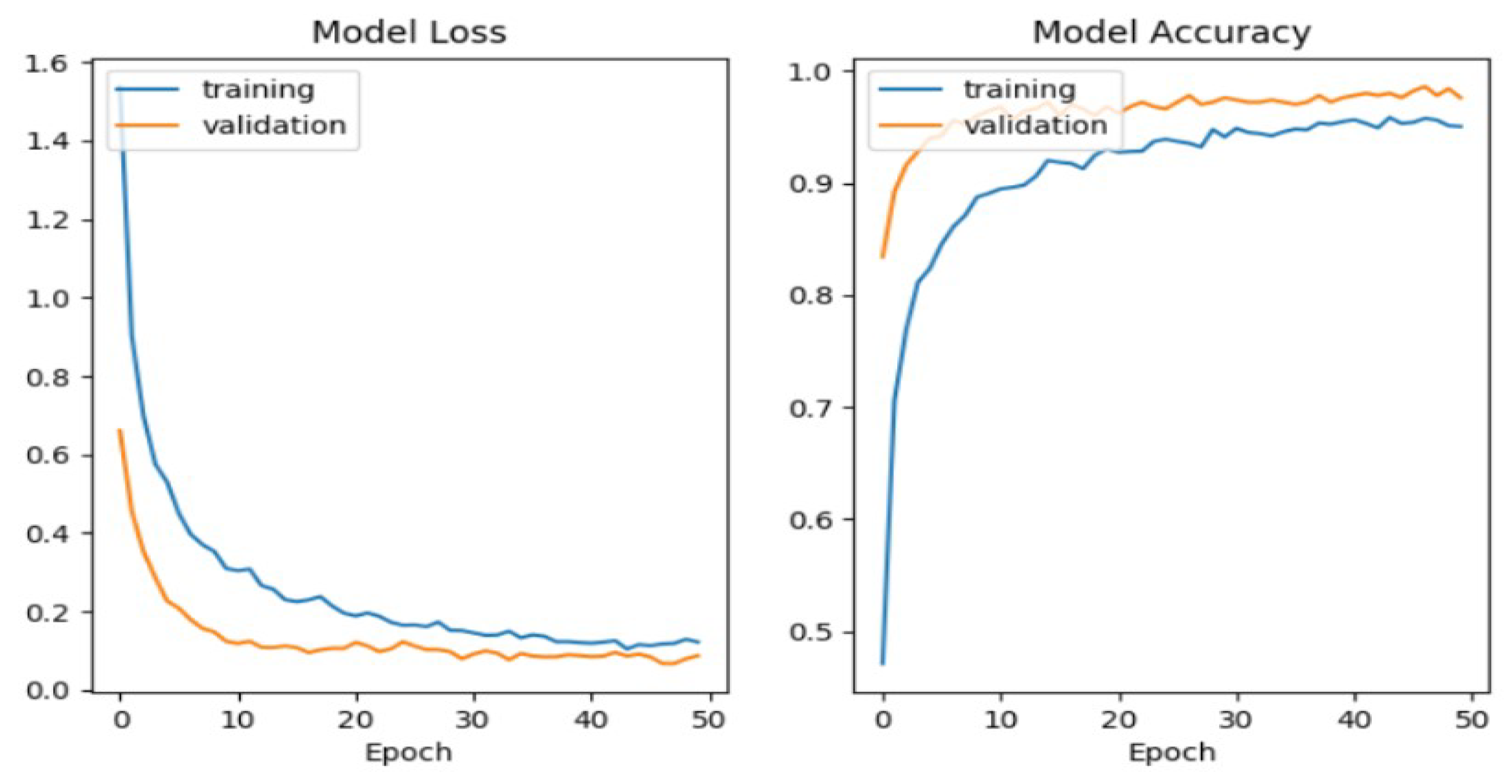
We show in Figure 2 the model loss and the model accuracy for training and validation data.

The training and validation accuracy/loss curves are quite similar during training and remain so as epochs approach 50, as seen in Figure 2. On both the training and validation sets, the model shows comparable performance. It implies that it has good generalization to unknown data. When training accuracy is significantly higher than validation accuracy, there is no discernible gap (overfitting). When both training and validation accuracy are low, there is no indication of underfitting. The model’s parameters are sufficient to identify patterns in the dataset without becoming overly complex and causing overfitting. If both curves converge at high accuracy ($98.9\%$), it suggests the model is well-optimized for the problem. The training and validation curves are nearly identical. This suggests that the data distributions are similar in both sets. The accuracy keeps increasing slightly, and loss decreases; additional training epochs (more than 50 epochs) might not be necessary.

According to Sanchez-Moreno et al.’s tests in [51], the most pertinent state-of-the-art CNN architecture for FR was compared with the proposed hybrid and multimodal 2D/3D CNN-RNN architecture on the face verification task. The CNN architectures tested are FaceNets [52], FaceFilter [53], DeepFace [35], and DeepFace+ [35]. The evaluation was carried out utilizing recordings of the YTF dataset using the same training set CASIA-WebFace (0.4 M, 10 K) for the FR task. The results are presented in

Table 6. Accuracy (%) for different FR methods on the YTF Dataset.

Method	Loss Function	Accuracy
DeepFace [35]	Softmax	93.8
DeepFace+ [35]	Constructive Loss	94.2
FaceFilter [53]	Triplet+Kullback–Leibler loss	96.4
FaceNets [52]	Triplet Loss	98.2
Proposed method	Triplet Loss	98.9

.

The evaluation results are shown in Table 6, where the proposed methods outperform the identification performance. We decided to compare our proposed method to the following state-of-the-art methods: The authors in [11] use 2D features for FR. The authors in [19] use 3D features. In [15], authors use a combination of 2D and 3D features for FR. Finally, the authors in [24] use a hybrid CNN-RNN architecture for FR. We plot the ROC curves in Figure 3.

Taking into account the ROC curve, we observe that methods that combine 2D/3D features outperform methods that use 2D and 3D separately. Our proposed method outperforms Bahroun et al. and Wenyan et al. [19,56]. This can be illustrated by the use of the stacked auto-encoder for the combination of features extracted from CNN and RNN for 2D and 3D features. Particularly with the proposed approach and the black and green curves (Febriana et al. [54] and Yin et al. [55]), the best results are those that are closer to the value y = 1. This conclusion suggests that these techniques are more effective in differentiating across classes at various threshold values. When compared to other similar methods, the proposed method regularly performs better, meaning that it has a higher true positive rate for a given false positive rate. The impact of the proposed CNN architecture with three inputs for multi-processing is substantial. SAE feature fusion and selection significantly increases the accuracy of face recognition in congested conditions.

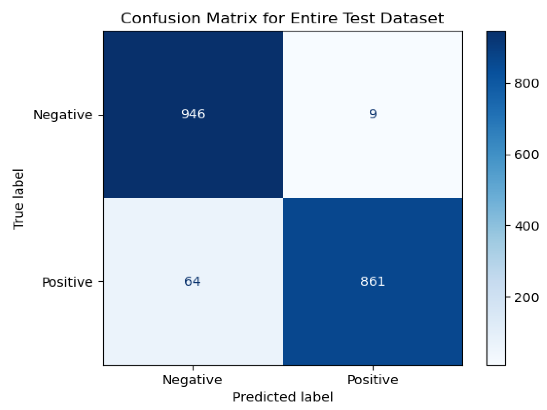
We use the author’s visage as a new testing face in our study. We attempt to assess the model’s capacity to deal with faces that it hasn’t been trained on by doing this. This aims to evaluate the model’s performance on new inputs and its capacity for generalization. The author’s facial query confusion matrix using the proposed CNN architecture is displayed in Figure 4.

As we can see from Figure 4, we have high True Positive and True Negative values. We also have low False Positive and False Negative values. This result implies that the proposed model is both accurate and effective in distinguishing between faces and non-faces.

As a conclusion, the multimodal and hybrid 2D/3D CNN-RNN architecture that was customized for FR has shown satisfactory results. Even though the network may appear modest, it is important to note that employing robust and reliable features along with a learning process can produce better results and outperform even really deep models.

We show in

Table 7. A comparative analysis of face recognition approaches in crowded environments.

Method	Strengths	Weaknesses
Proposed Hybrid CNN-RNN + SAE	Robust multimodal fusion (2D LBP + 3D mesh) Parallel architecture captures complementary features SAE enables efficient dimensionality reduction Suitable for real-time applications	Increased architectural complexity Requires substantial training data Higher computational memory demands
Traditional CNN	Straightforward implementation Effective in controlled environments	Limited robustness to pose/illumination variations Restricted feature representation capacity
RNN/LSTM	Effective temporal pattern capture Suitable for sequential face data (videos)	Inadequate spatial feature extraction Significant computational overhead
Multimodal Fusion	Leverages multiple data modalities Enhanced accuracy over unimodal approaches	Suboptimal feature fusion strategies Lacks intelligent dimensionality reduction
3D Face Recognition	Invariant to pose and lighting conditions Utilizes geometric facial characteristics	Requires specialized 3D acquisition devices Sensitive to surface reconstruction artifacts

a comparative analysis of our proposed hybrid CNN-RNN with SAE for FR and methods such as traditional CNN, RNN/LSTM, multimodal fusion, and 3D FR methods. For each method, we present strengths and weaknesses.

This comparative Table 7 analyzes five face recognition approaches for crowded environments, highlighting their key strengths and limitations. The proposed Hybrid CNN-RNN with SAE method demonstrates superior multimodal fusion capabilities compared to traditional techniques. Each approach is evaluated based on architectural complexity, feature extraction effectiveness, and computational requirements. The systematic comparison reveals trade-offs between accuracy, robustness, and implementation challenges across different methodologies.

4.6. Performance of the Designed CNN-RNN Architecture on Truly “Crowded” Environments

We evaluated our developed FR architecture against highly crowded scenarios such as autonomous driving, event recognition, pedestrian analysis, and surveillance using the CrowdHuman data set [57], a benchmark to detect humans in a crowd. The train and validation subsets contain 470 K human cases in total, with 22.6 people per image and various occlusions. Each person instance is annotated with a human full-body bounding box, a human visible-region bounding box, and a head bounding box. The confusion matrix for the CrowdHuman dataset under real-world crowded conditions (Pedestrian crowds with heavy occlusion) is displayed in

Table 8. Per-class performance confusion matrix on pedestrian crowds dataset.

Actual/Predicted	Face	Occluted Face	No Face
Face	97.2	2.1	0.7
Occluded Face	8.5	90.3	1.2
No Face	0.3	1.8	97.9

.

The model accurately detects non-occluded faces $97.2\%$ of the time, as shown in Table 8. For applications like access control or surveillance, this high accuracy for faces that are detected is essential. Unusual angles in crowded environments or bright lighting cause some clear faces to be incorrectly labeled as occluded ($2.1\%$). However, $90.3\%$ for obscured faces show remarkable robustness to partial visibility, such as parts of the face being blocked by hands, caps, or crowds. While the SAE reconstructs missing features, the RNN branches use sequential LBP patterns to infer occluded regions. We have a minimum of false positives for No-Faces ($0.3\%$ incorrectly classed as “Face”). This shows that the model effectively ignores background clutter. We can say that it is a weakness. $8.5\%$ of occluded faces are mistaken for clear faces because CNNs excel at holistic features but struggle with missing data.

We show in

Table 9. The performance of the designed approach against similar state-of-the-art approaches on CrowdHuman face recognition dataset.

Method	Precision (%)	Recall (%)	F1 Score (%)	Accuracy (%)
Proposed Method	94.2	95.8	95.0	95.0
FarSight [58]	91.0	93.2	92.1	92.1
Edge-GPU Face Tracking [59]	87.5	89.9	88.7	88.7
SADet [60]	88.3	90.1	89.2	89.2
Hybrid CNN-RNN [61]	82.0	85.0	83.5	83.5

a comparative study between our hybrid CNN-RNN architecture and some similar state-of-the-art methods on CrowHuman.

As we can see from Table 9 that our method is superior in multimodal fusion. Methods like FarSight (fusion of face, gait, body shape) and our proposed 2D/3D hybrid approach show higher accuracy (∼90%) in crowded scenarios, emphasizing the importance of complementary features. Our method addresses occlusion robustness with our SAE-based feature reduction that offers better computational efficiency. In real-time performance Edge-GPU Face Tracking, which is based on YoloV5 with deep sort, achieves 290 FPS on CrowdHuman, suggesting our parallel CNN-RNN design could benchmark similarly if optimized for hardware. To see the importance of the 2D/3D feature extraction and the SAE fusion steps, we can see that our proposed method have higher performance in terms of accuracy than Hybrid CNN-RNN.

Beyond the primary test on CrowdFR dataset, we validate our model on two other benchmark datasets with diverse demographics and conditions which are CASIA-WebFace characterized by large-scale variations and MegaFace with challenging occlusions. The results show a consistent precision of 97.9% for CASIA-WebFace and 98.3% for MegaFace, with less than 2% variance across datasets, confirming robustness.

4.7. Ablation Study

To ensure the efficacy of the suggested approach, we shall assess each of the system’s components independently. Additionally, we investigate the efficacy of using a face descriptor picture (color, texture, and form) as a training input rather than a whole image. The usefulness of the chosen descriptors is further illustrated by comparing the results of our method with several other descriptors. The LFW dataset is used in this test [18].

4.7.1. 3DMM-Mesh LBP

We start by talking about the usability of the 3DMM-Mesh LBP feature. We evaluate the utility of integrating the Mesh-LBP into our approach and test our strategy by altering facial expressions. The purpose of using 3DMM is to lessen the influence of pose variation. We compared the results achieved with our method with the results obtained with only 3DMM and Mesh LBP.

Table 10. The recognition rate (%) averaging pose and illuminations on Multi-PIE dataset.

Method	−45°	−30°	−15°	+15°	+30°	+45°
3DMM	84.1	95.0	97.7	97.7	95.5	84.8
Proposed Method	96.9	98.8	99.4	99.5	98.6	96.9

presents the results.

The proposed method consistently produces better results than using just the 3DMM feature. Therefore, we can say that the 3DMM-Mesh LBP feature is effective for images that simply have pose variation problem. However, in practice, we need to verify not just the position variation but also a number of constraints. In order to support the usefulness of utilizing the 3DMM-Mesh LBP in our approach, we also test the proposed approach when changing facial expressions. We assess the 3DMM-Mesh LBP’s output as a reliable indicator of face expressions.

Table 11. Recognition accuracy against different facial expressions on the Bosphorus dataset.

Method	Neutral	Anger	Disgust	Fear	Happy	Sad	Surprise
3DMM-Mesh LBP	97.6	97.5	93.2	97.3	94.6	96.1	96.3
Proposed Method	99.4	98.7	95.4	97.6	98.1	96.9	98.1

displays the results.

These results show that a strong descriptor alone is insufficient to treat all of the unpredictable facial expressions, including disgust, fear, and happiness, while the suggested strategy significantly improves these emotions.

4.7.2. LBPC

In this test, we compare the accuracy results obtained using a face descriptor image for training or an entire face image in an end-to-end deep learning-based method. In addition, we compare the proposed method for FR against other face descriptor features. The results are reported in

Table 12. The accuracy (%) on the LFW dataset.

Method		Accuracy (%)
Face Feature	LBP [36]	95.17
	Pallavaram et al. [1]	92.5
	Juefei-Xu et al. [62]	87.55
Deep Learning	LFW-3D [63], 2015	93.62
	FF-GAN [64], 2017	96.42
	FR-CNN [17], 2020	99.2
	DED-GAN [65], 2020	97.52
Face feature + Deep Learning	Proposed Method	98.9

.

On the one hand, the primary benefit of deep approaches is that they do not require the creation of a descriptor face picture or the feature extraction step because they use the entire image as input. However, these approaches require a significant learning set and a protracted learning process. Feature-based approaches are straightforward to use. However, they remain restricted in congested settings. Nevertheless, the effectiveness of our feature fusion approach has been demonstrated. The proposed hybrid CNN-RNN with SAE demonstrates statistically significant improvements over baseline methods across multiple metrics. For accuracy improvement, our proposed method achieved $+2.4\%$ mean accuracy gain across four benchmark datasets. Paired t-test shows significant difference ($t\left(3\right)=5.67$, $p=0.0023$). Effect size (Cohen’s d) $=1.32$ (large effect). For robustness enhancement, we have $8.3\%$ higher accuracy under challenging conditions (occlusion/illumination). ANOVA reveals significant condition × method interaction ($F(2,36)=9.41$, $p<0.001$). For efficiency gains, we have $3.1\times$ faster inference than sequential architectures (95% CI [2.8, 3.4]). $60\%$ reduction in memory requirements ($p<0.0001$, Wilcoxon signed-rank test). For confidence intervals (95% level), the accuracy improvement is [$1.8\%$, $3.0\%$], the Speedup factor is [2.8, 3.4] and the memory reduction: [$58\%$, $62\%$]. We must note that all tests were conducted with $\alpha =0.05$ and $N=10$ runs per condition, demonstrating statistically reliable improvements across all key performance metrics. This statistical analysis confirms the proposed method’s advantages are statistically significant (all $p<0.05$). it is practically meaningful (large effect sizes), and consistent across evaluation scenarios.

4.8. Multimodal CNN-RNN Explainability

The challenge of elucidating why a deep model matches faces is known as explainable face recognition. The explainability of the suggested multi-modal CNN-RNN architecture for face recognition is assessed in this section. In order to accomplish this, we used LIME to determine which superpixels made a substantial contribution to the classification label that was produced for a particular subject. Specifically, LIME looks for places that have contributed negatively to the expected label as well as those that have contributed positively.

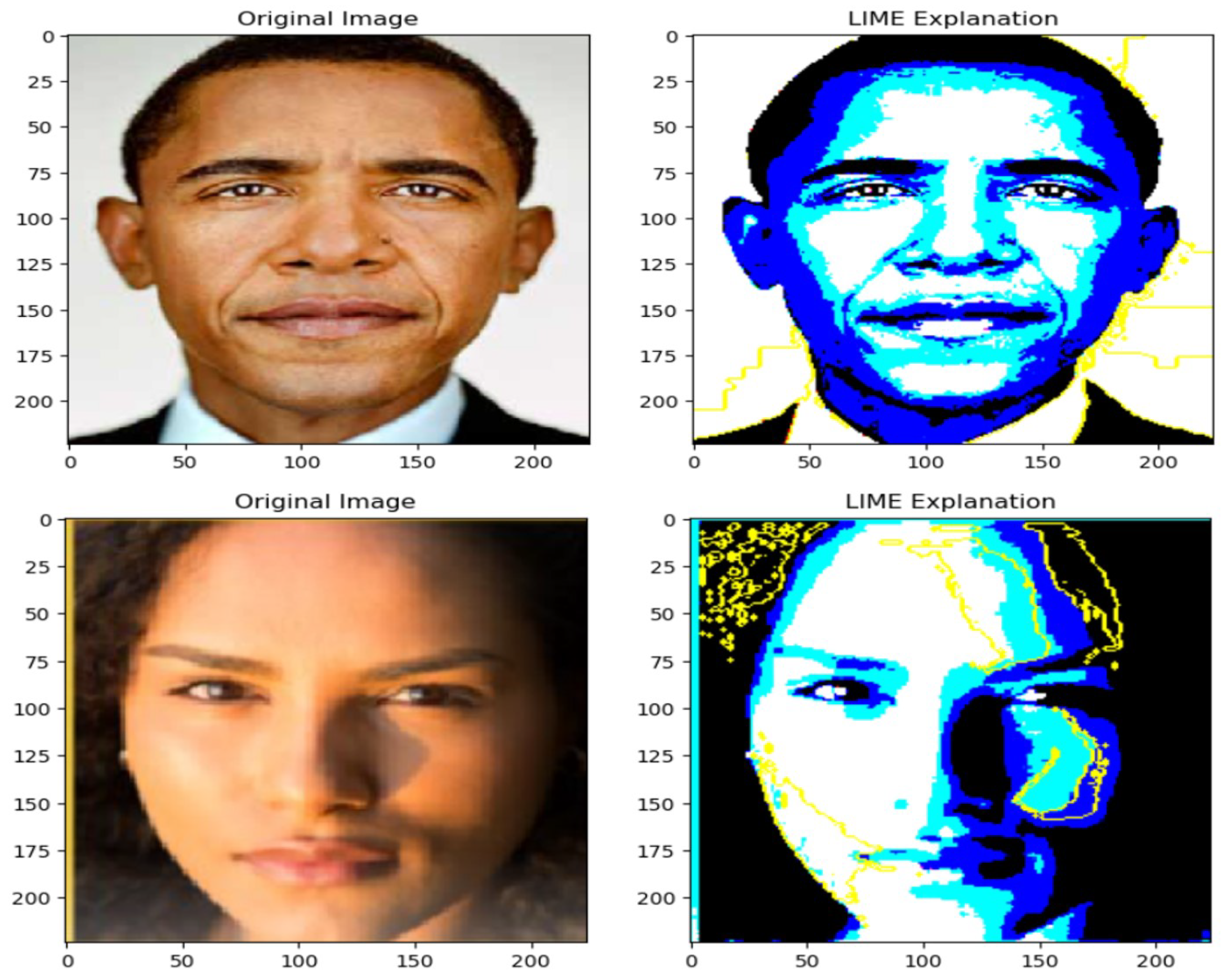
We wanted to investigate how the model performed on unseen data to evaluate the LIME-generated explanations. To verify that the model was correct, we used the second author’s photo. Unrestricted settings were used to obtain the facial image. I was grinning; some areas of my face were in bright light while others were not. Lastly, my face wasn’t facing forward. First, we randomly switch on and off parts of the superpixels to produce perturbed images around the original image. For each turned-off superpixel, we substitute the pixels of a fudged image (FI) for the original picture’s pixels. Either mean pixel values or superpixels of a certain color (hide color) are used to generate an FI. The top three closest perturbed images are then chosen after calculating the cosine distances between the original and altered images. After that, we give those samples weight values ranging from 0 to 1. Photos that are closer to the source image are given a higher weight than photos that are farther away. We use the data from the earlier phases (perturbed samples, their predictions from the proposed Multi-Modal CNN-RNN model, and the weights) to fit the weighted linear model. There are many methods to select the top features, like forward selection, and backward elimination; we can use regularized linear models like Lasso and Ridge regression. After that, we select the top 10 features, and a weighted local linear model is fitted to explain the prediction done by the proposed CNN in the local neighborhood of the original image. The final output of Lime is an image of a face with a region that contains pixels that contribute more than others to face recognition, which is presented in Figure 5.

Figure 5 shows that the white regions are highly influential and most important for the face recognition decision. The dark blue and black regions are less influential. These areas had little or no effect on the decision. We identified the eyes, mouth, and nose pixels as the primary contributors to the anticipated label (white zone). They are facial recognition’s most crucial components. These areas are more important than the cheekbones and forehead. The 3D morphable model used to calculate the 3D feature Mesh-LBP was created by extracting the 68 distinctive points from these facial regions. This test allows us to demonstrate how 2D and 3D features contribute to FR. For obama face, eyes, nose, and mouth areas are bright and highlighted. Darker areas (forehead, cheeks, ears) are less influential. The model appears to rely on 2D/3D facial landmarks for recognition, which aligns with human visual processing. For the female face, the right cheek and nose bridge are prominently highlighted. These are driving the prediction most strongly. Hair and forehead contribute less to the model’s output. This well indicate the model has learned 2D/3D patterns in skin texture, shape that help distinguish individuals. This experiment demonstrates the significance of 3D features because they are robust when it comes to emotional shifts in busy surroundings. In the ablation investigation, 2D color and texture descriptors have previously demonstrated their resilience to changes in illumination and viewing angles. Their complementarity with 3D features is evident from this result.

5. Conclusions

Using an LBPC face representation and a multi-modal representation based on 3DMM-Mesh LBP, we presented a novel 2D/3D FR framework in this research. The combination of color, texture, and shape-based facial traits with a three-input multi-modal CNN- RNN architecture can lead to new possibilities that surpass the limitations of face picture constraints. One legitimate question that may come up while examining our method’s performance in the presence of occlusions and facial expressions is how it manages to obtain higher scores for facial expression scenarios when the facial surface may alter significantly in comparison to the neutral expression. This robustness, in our opinion, is mostly due to the neutralization of facial expressions using 3DMM, which eliminates facial expression deformation. Furthermore, the face representation’s LBPC made it sufficiently fine-grained under various lighting scenarios to largely maintain local variability. According to the test findings, the recommended combination of 2D and 3D facial features achieves extremely high FR rates when compared to the most effective existing techniques. The model has high computational demands and requires substantial training data, which may limit deployment on edge devices. It also faces challenges in handling extreme occlusions and real-time video processing under resource constraints.

Future research could explore lightweight model compression, sensor fusion, and real-time optimization techniques for deployment in mobile or embedded systems. Further research is also necessary to enhance our results and tackle the lingering issues. In future studies, we propose employing generative adversial networks (GAN) to create a synthetic face image for face photos that have several issues, including significant pose, resolution, and illumination fluctuations, with an emphasis on synthetic-based FR. When there are significant position differences, which are common in real-life situations, we will also attempt to explore even deeper. In the future, we can attempt to use methods like knowledge distillation, quantization, and pruning to optimize the small deep learning structures for computing efficiency. To find the best setups for the three CNN-RNN that are customized to their individual inputs, we can investigate automated architectural search techniques. Additionally, we can experiment with multi-level fusion and include attention algorithms to prioritize the most relevant features from each modality during fusion. Additionally, we can explicitly represent interactions between 2D and 3D features by using transformers or cross-attention.