Gait-Based Parkinson’s Disease Detection Using Recurrent Neural Networks for Wearable Systems

Abstract

Parkinson’s disease is one of the neurodegenerative conditions that has seen a significant increase in prevalence in recent decades. The lack of specific screening tests and notable disease biomarkers, combined with the strain on healthcare systems, leads to delayed detection of the disease, which worsens its progression. The development of diagnostic support tools can support early detection and facilitate timely intervention. The ability of Deep Learning algorithms to identify complex features from clinical data has proven to be a promising approach in various medical domains as support tools. In this study, we present an investigation of different architectures based on Gated Recurrent Neural Networks to assess their effectiveness in identifying subjects with Parkinson’s disease from gait records. Models with Long-Short term Memory (LSTM) and Gated Recurrent Unit (GRU) layers were evaluated. Performance results reach competitive effectiveness values with the current state-of-the-art accuracy (up to 93.75% (average ± SD: 86 ± 5%)), simplifying computational complexity, which represents an advance in the implementation of executable screening and diagnostic support tools in systems with few computational resources in wearable devices.

1. Introduction

Parkinson’s disease (PD) is a progressive neurodegenerative disorder that significantly impacts an individual’s motor abilities and daily functioning. It is characterized by a variety of symptoms, including tremor, muscle rigidity, bradykinesia, and impaired balance and coordination. According to the World Health Organization (WHO) [1], PD affects approximately 1–2 per 1000 people currently, with its incidence increasing with age. Globally, statistics indicate that the incidence of disability and mortality associated with PD exceeds that of any other neurological pathology. Since 2000, the prevalence of PD has doubled, and WHO estimates report an increase of 81% and more than 100% in disability-adjusted deaths and deaths caused by this neurological disorder. Furthermore, the stigma of the disease and the psychological and logistical burdens placed on the families of the patients highlight the urgent need for improved healthcare and social support systems, including more efficient diagnostic processes.

Recent studies have shed light on various aspects of Parkinson’s disease, revealing intriguing insights into its complex nature. For example, emerging research suggests a potential link between gut health and PD. The gut-brain axis, a bidirectional communication system between the gastrointestinal tract and the brain, has gained attention in PD research [2]. Researchers propose that changes in the gut microbiota could impact the onset and progression of PD, suggesting that this axis could offer novel insights and therapeutic targets for the disease.

Furthermore, the role of neuroinflammation in PD has attracted increased attention. Chronic brain inflammation, primarily driven by cells such as microglia and astrocytes, plays a crucial role in PD pathology [3]. This inflammation, often initiated by misfolded alpha-synuclein proteins, contributes significantly to the degeneration of neurons critical for motor control. Developing therapeutic strategies that target this inflammation could potentially slow or stop the progression of PD.

The exact causes of Parkinson’s disease are not yet fully understood, but are believed to stem from a combination of genetic and environmental factors [4]. Researchers have made significant progress in understanding the underlying mechanisms and pathophysiology of the disease, leading to the development of various diagnostic and treatment approaches [5,6]. Non-pharmacological interventions have also been systematically reviewed in the literature, highlighting the relevance of tailored therapeutic strategies in PD management [7]. Despite these advances, the diagnosis of PD still relies heavily on clinical evaluations considering symptoms, medical history, and physical examination findings [8]. The absence of a definitive diagnostic test complicates early detection and timely intervention of the disease [9].

The challenge of early diagnosis has sparked innovative research in the field of medical technology. More efficient and accurate diagnostic methods are needed to facilitate early identification of the disease [10]. Currently, advances in therapeutic interventions and research into new technologies aim to revolutionize early diagnosis and treatment strategies [11]. In particular, Artificial Intelligence (AI), and particularly Machine Learning models, have emerged as a promising field, offering substantial support in diagnosis and screening applications.

Artificial intelligence’s role in healthcare has significantly expanded, with Machine Learning, especially Deep Learning models, playing a pivotal role in analyzing complex datasets. These models have been effectively applied in various domains, including medical imaging [12,13], audio analysis [14], and biomedical signal processing [15,16]. The use of DL models can enhance diagnostic precision and operational efficiency, empowering healthcare professionals to make more informed decisions.

Gated Recurrent Neural Networks (RNNs), which encompass architectures like Long-Short Term Memory (LSTM) and Gated Recurrent Unit (GRU), have demonstrated potential across a range of medical applications. Their effectiveness as classifiers for medical time series data [17,18] indicates that they could be particularly valuable in the early diagnosis of Parkinson’s disease, where timely and accurate detection is crucial.

This research study aims to analyze the effectiveness of AI models based on Gated RNNs as diagnostic support tools for early diagnosis of Parkinson’s disease utilizing plantar insole pressure sensors. By analyzing subtle alterations in gait and plantar pressure patterns, this system aims to accurately identify Parkinson’s disease in its early stages. Such an approach could greatly improve early detection and intervention efforts, potentially leading to significant improvements in patient outcomes and quality of life.

Advancements in wearable technology have revolutionized the monitoring and management of Parkinson’s disease. Equipped with sensors to track movement patterns and vital signs, wearable devices facilitate continuous health monitoring beyond the confines of clinical settings. This technology not only aids in the early detection of motor symptoms, but also facilitates the development of customized treatment plans [19]. Integrating these devices with AI algorithms could lead to real-time patient-specific management of Parkinson’s disease, enhancing treatment efficacy.

The remainder of the manuscript is organized as follows. Section 2, Related Works, reviews the existing literature pertinent to the use of Gated Recurrent Neural Networks in medical applications, particularly for Parkinson’s disease. Section 3 describes the materials and methods used in this study, including the dataset for training and evaluation, the specifics of the two types of RNN architectures employed, the architectures considered, and the criteria for evaluating their effectiveness. Section 4 presents the results and discussion of the Deep Learning models that were trained. Finally, Section 5 concludes the paper with a summary of the findings and discusses potential avenues for future research.

2. Related Works

Parkinson’s disease (PD) detection using gait analysis has been investigated through various approaches. This section reviews the most recent studies that have utilized advanced supervised machine learning algorithms to enhance detection performance.

Ertuğrul et al. used shifted one-dimensional local binary patterns (Shifted 1D-LBP) to detect PD from gait data [20]. This approach focused on detecting local changes in time-ordered signals, by adjusting neighbor positions for improved pattern extraction. From these patterns, various supervised learning models were trained to further analyze and classify the data. The most promising results were achieved with multilayer perceptron (MLP) models, which demonstrated an accuracy of 88.9%.

Zhao et al. introduced a hybrid spatio-temporal model combining Long Short-Term Memory (LSTM) and convolutional neural network (CNN) layers to detect PD from Vertical Ground Reaction Force (VGRF) data [21]. This model achieved high classification performance, with a recall rate of 98.61%. However, the use of various deep learning layers can lead to increased execution times.

Another approach was presented by Asuroğlu et al., which consisted of a Locally Weighted Random Forest (LWRF) model that applied regression analysis to numerical features extracted from ground reaction force (GRF) signals. Their approach showed superior correlation coefficients and error metrics in PD detection compared to other models, achieving high accuracy [22]. However, a drawback of this model is its reliance on the extraction of several computationally expensive features and the execution of multiple decision trees, which can impact response times.

El Maachi et al. proposed a 1D-Convnet model for PD detection and severity prediction, which processed signals from foot sensors and demonstrated state-of-the-art performance with an accuracy of 98.7% [23]. Another contribution in 2020 was Alkhatib et al.’s, who designed three CNN architectures of varying complexity, achieving the best classification results with an intermediate-complexity model featuring parallel convolutional layers [24]. Both contributions highlight the effectiveness of the proposed models and their tolerance to noise in signals. However, similar to other aforementioned contributions, these are computationally intensive models, which consequently result in higher computational demands.

In this context, our contribution lies in analyzing the performance of models composed solely of recurrent neural network layers for Parkinson’s disease detection through gait analysis. RNNs have been successfully applied to various signal processing challenges, demonstrating high performance and efficiency. In particular, these models can be implemented on low-power devices, offering potential for real-time data management directly from wearable sensors. This approach could provide an accessible solution for the continuous monitoring and early detection of Parkinson’s disease in everyday settings.

3. Materials and Methods

The primary objective of this research is to examine the feasibility of developing a diagnostic tool for detecting signs of Parkinson’s disease by analyzing user gait data collected via a wearable device. This study focuses on using RNNs enhanced with a final classification layer. These are supervised learning algorithms that require a robust dataset consisting of accurately labeled samples, which facilitates effective learning and validation.

To evaluate the performance of these trained models, we employed a variety of metrics, complemented by techniques to minimize bias and ensure the validity of the results. These measures are crucial for accurately assessing the robustness of the architectures utilized. This section presents a detailed explanation of all these aspects.

3.1. Classifiers

This section presents the main characteristics of Gated RNNs and describes the architectures analyzed in the study, as well as the common training functions selected for optimizing classification performance.

3.1.1. Gated Recurrent Neural Networks

Gated RNNs are a variant of traditional RNNs specifically designed to address the issues of vanishing and exploding gradients, which commonly occur when processing long data sequences [25,26]. They achieve this by incorporating internal gating mechanisms that regulate the flow of information through the network. The two predominant architectures within Gated RNNs are LSTM networks, proposed by [27], and Gated Recurrent Units (GRU), introduced by [28]. Both LSTM and GRU utilize sigmoid and hyperbolic tangent activation functions within their gates to control which information is passed through, thereby managing what is stored in and retrieved from the network’s memory. While both serve a similar fundamental purpose of handling long-term dependencies, they differ in their internal structure: LSTM networks typically employ three gates (input, forget, and output gates) and a cell state, whereas GRU networks are a more simplified version with two gates (reset and update gates) that merge the hidden state and cell state into a single hidden state. Consequently, LSTM networks are generally more computationally complex than GRU networks. However, depending on the specific problem, GRU can offer comparable or even superior performance with greater computational efficiency.

3.1.2. Architectures Considered

In this study, deliberately simple Deep Learning architectures were chosen to effectively address classification challenges. It was decided that the hidden layers would consist solely of recurrent cells (LSTM or GRU) to maintain architectural simplicity and focus. The models considered were configured with one or two recurrent layers, each using exclusively LSTM or GRU cells. This approach was taken to avoid the complexities and potential inefficiencies that might arise from mixing different types of recurrent layer in a single model. To further enhance the model’s training convergence and stability, batch normalization techniques were systematically implemented across the recurrent layers. This method helps to normalize the input to each layer within a minibatch and is crucial for accelerating the training process while improving model performance. In addition, to combat the risk of model overfitting to training data—a common issue in neural network training—a dropout technique was applied consistently to each of the hidden layers.

Given the binary nature of the classification task in this context, where the goal is to discern whether a subject has Parkinson’s disease based on gait analysis, each model architecture was designed with a single output node. This node was implemented with a sigmoid activation function. The loss function employed for optimizing the models was Binary Cross-Entropy. The Adam optimizer was selected to adjust the weights during the training phase. The selection of these hyperparameters and functions, which are well-established in Deep Learning literature, was intended to ensure the robustness and generalizability of the developed models. In addition, these choices were designed to enable high accuracy in distinguishing between individuals with and without Parkinson’s disease. Importantly, these characteristics are well-supported in deep learning frameworks optimized for embedded systems, making them suitable for integration into wearable devices.

3.2. Dataset

For the Parkinson’s identification study using machine learning models, we utilized a dataset, which was then adapted for the proper training and evaluation of the architectures considered in the study. In this section, we discuss this process in detail.

3.2.1. Gait in Parkinson’s Disease Dataset

The research described in this article used the “Gait in Parkinson’s Disease” dataset, sourced from the PhysioBank repository [29]. This specific dataset is comprehensive, comprising 306 individual files that encapsulate data collected from 164 participants. These participants were equipped with 16 force sensors evenly distributed in two shoes, with eight sensors embedded in each shoe. During the data collection phase, participants were instructed to perform gait tests while walking on a flat surface for approximately two minutes. Throughout these tests, the sensors recorded data at a frequency of 100 Hz, capturing the force measurements from each sensor.

The participants in this dataset are categorized into two distinct groups: 92 individuals diagnosed with idiopathic Parkinson’s disease and 72 control subjects, derived from three separate research studies. The average age among the Parkinson’s disease group is 66.3 years, and males constituted approximately 63% of this group. The control group closely mirrors this demographic, with an average age also of 66.3 years, but with a slightly lower male representation at 55%. Each dataset file records sensor readings from both feet, aggregating the force outputs from the eight sensors located in each shoe.

The force sensors used in this study, labeled R1 through R8 for the sensors on the right foot and L1 through L8 for those on the left foot, were manufactured by Ultraflex Computer Dyno Graphy, Infotronic Inc. Throughout the duration of the studies, data collection was performed multiple times for each subject, and some participants were asked to perform various gait tests to explore different styles and patterns of walking. However, for the purpose of training predictive models, only data derived from standardized gait tests were selected for each participant. This resulted in a compilation of 164 distinct files, 92 of which correspond to participants diagnosed with Parkinson’s disease, accounting for 56% of the total number of participants involved. This selective approach to data usage was strategic, with the aim of improving the consistency and accuracy of the dataset for further analysis and model training.

3.2.2. Adaptation and Split Process

Before partitioning, the selected data underwent a normalization process to ensure uniformity and mitigate potential biases and in model training and evaluation. Following this preparatory step, the data were divided into three distinct subsets: the training set, the validation set, and the test set. The allocation of data to these sets was performed in a random, yet representative manner, which is crucial for maintaining the integrity of the modeling process. The chosen distribution ratio was 75-15-10; this configuration allocated 75% of the dataset to the training set, 15% to the validation set, and the remaining 10% to the test set.

This practice, known as the Train-Validation-Test split, is designed to evaluate and refine the model performance while preventing evaluation bias. The training set is used to adjust the model parameters by training with the backpropagation algorithm. The validation set, meanwhile, is used not for internal model tuning but to guide the selection of optimal hyperparameter values by analyzing performance metrics.

The test set serves as the final evaluation phase, used to measure the performance of the fully trained model using data that had not been used in any previous phase of training or hyperparameter tuning. This provides a robust and objective assessment of the model’s performance.

As a result, the division of the 164 files is as follows:

• Training set: 124 files, of which 68 correspond to subjects with Parkinson’s disease
• Validation set: 24 files, of which 16 correspond to subjects with Parkinson’s disease
• Test set: 16 files, of which 8 correspond to subjects with Parkinson’s disease.

To input temporal sequences into the recurrent neural network, the data was sampled. This involved dividing the data into segments that represent gait units indicative of Parkinson’s disease. The data files were segmented into samples of a specified length with overlap. A 2-second window was determined to be adequate to cover one full gait cycle and part of the next. This resulted in a sample size of 200 temporal instances. An overlap of 50% was used in the sampling process to preserve time-dependent information and maximize the data available for training.

All samples were labeled according to the diagnosis associated with the participant, resulting in each sample having dimensions of 200 rows by 16 columns. Depending on the length of the files, various numbers of samples were produced, with the mode number of samples per file being 120, found in 111 files, representing 68% of the recorded activities. The total number of samples obtained from the dataset is 18,217.

After the data splitting and sampling mentioned above, the following proportions were observed in the different sets.

• Training set: 13,829 samples from 124 files, with 54.8% of files from PD subjects. This subset contains 7873 samples from Parkinson’s subjects, representing 56.9% of the total training samples.
• Validation set: 2602 samples from 24 files, with 66.6% of files from PD subjects. This subset contains 1747 samples from Parkinson’s subjects, representing 67.1% of the total validation samples.
• Test set: 1786 samples from 16 files, with 50% of files from PD subjects. This subset contains 905 samples from Parkinson’s subjects, representing 50.6% of the total test samples.

A summary of the distribution of the subjects and the signals collected is presented in

Table 1. Dataset distribution for each subset. ‘Co’: Control group, ‘Pt’: Patients with Parkinson.

	Data Registers		Samples
Subset	Co	Pt	Co	Pt	Total
Training	56	68	5956	7873	13,829
Validation	8	16	855	1747	2602
Test	8	8	881	905	1786
Total	72	92	7692	10,525	18,217

. This detailed configuration ensures that the sample composition in each subset closely mirrors the composition of the file registers in their respective subsets prior to sampling, maintaining consistency throughout the study.

3.3. Evaluation Metrics

To evaluate the effectiveness of the classification results of a classifier, the most common metrics are used: accuracy (most used metric), sensitivity (known as recall in other works), specificity, precision, and F1_$score$ [30]. To this end, the classification results obtained for each class are tagged as “True Positive” (TP), “True Negative” (TN), “False Positive” (FP), or “False Negative” (FN). According to them, the high-level metrics are presented in the following equations.

$$Accuracy=\sum _c{\displaystyle \frac{T{P}_c+T{N}_c}{T{P}_c+F{P}_c+T{N}_c+F{N}_c}},c\in classes$$

(1)

$$Precision=\sum _c{\displaystyle \frac{T{P}_c}{T{P}_c+F{P}_c}},c\in classes$$

(2)

$$Recall=\sum _c{\displaystyle \frac{T{P}_c}{T{P}_c+F{N}_c}},c\in classes$$

(3)

$$Specificity=\sum _c{\displaystyle \frac{T{N}_c}{T{N}_c+F{P}_c}},c\in classes$$

(4)

$$F{1}_{score}=2\ast {\displaystyle \frac{precision\ast sensitivity}{precision+sensitivity}}.$$

(5)

About those metrics:

• $Accuracy:$ all samples classified correctly compared to all samples (see Equation (1))
• $Precision$: proportion of values classified as “true positive” in all cases that have been classified as it (see Equation (2))
• $Recall$ (or Sensitivity): proportion of values classified as “true positive” that are correctly classified (see Equation (3))
• $Specificity$: proportion of “true negative” values in all cases that do not belong to this class (see Equation (4)).
• $F{1}_{score}$: Consider two of the main metrics (precision and sensitivity), calculating the harmonic mean of both parameters (see Equation (5)).

We also consider the ROC curve to assess the model’s performance. The ROC curve is a graphical representation illustrating the ability of the classification model to distinguish between positive and negative classes as the classification threshold varies. It is obtained by plotting the true positive rate (recall) against the false positive rate (1-specificity).

An ideal model would have a true positive rate of 1 and a false positive rate of 0, resulting in a curve that rapidly approaches the upper left corner of the graph. On the other hand, a model that cannot distinguish between positive and negative classes would have an ROC curve that resembles a diagonal line. In this context, the area under the curve (AUC) is a metric that summarizes the discriminative power of the model. It ranges from 0 to 1, where a value of 1 indicates a perfect model, and a value of 0.5 indicates a model with no discrimination ability better than chance. The higher the AUC value, the better the model classification performance.

The above metrics are standard in machine learning evaluation. Therefore, the classifier systems developed in this work were evaluated using all the metrics detailed in this subsection.

3.4. Optimization Process

To obtain the best classifier for the system, an optimization process based on two steps was implemented: In the first step, a global search was performed, involving multiple training runs with different hyperparameter variations for each classifier; and in the second step, the robustness of the best models was tested using a cross-validation technique. After this process, the best classifier is compared to previous work.

3.4.1. Model Optimization

In a first phase, the considered architectures were trained and evaluated using a combination of values for different hyperparameters. These hyperparameters included the number of nodes in the recurrent layers, the batch size, defined as the number of samples processed before the model’s weights are updated, the learning rate, which determines the step size for weight updates in the model, and finally, the dropout rate applied to each hidden layer. The specific hyperparameter ranges used in this study were based on previous studies that successfully applied similar LSTM and GRU architectures to gait analysis using accelerometer signals [31].

Table 2. Hyperparameters’ values.

Parameter	Values
Learning rate	0.0001, 0.001, 0.002, 0.005
Batch size	8, 16, 32, 64
Number of nodes	8, 16, 32, 64
Dropout (1st layer)	0.1, 0.2, 0.3, 0.4, 0.5
Dropout (2nd layer)	0.1, 0.2, 0.3, 0.4

shows the different values considered for each hyperparameter. A grid search approach was employed to identify the optimal combination that yielded the highest accuracy and stability.

3.4.2. Cross-Validation

Secondly, based on the results of the first stage, the robustness of the selected architecture was assessed by applying K-fold cross-validation. This technique involves partitioning the dataset into K distinct subsets, known as folds. Each subset is sequentially used as a test set once, while the model is trained on the combined remainder of the k − 1 folds. This process requires K training iterations and K evaluations, where each evaluation is based on predefined performance metrics. The process of data partitioning is depicted in Figure 1. The outcomes from these iterations were then averaged to compute a consolidated estimate of the model’s overall performance. This method is widely used not only for robust model evaluation but also to ensure that the performance metrics are not biased by the specific manner in which the data are divided between training and testing sets.

To implement the cross-validation, data were extracted from both training and validation subsets. Applying this methodology with K = 6, this approach yielded six sets of results for both accuracy and recall metrics for each of the four classifiers developed during the first phase of the study. This systematic testing across multiple folds provides a thorough validation of the classifier’s performance and reliability across different data partitions, thus enhancing confidence in the generalizability of the model’s predictions.

4. Results and Discussion

The hyperparameter optimization results indicate that a high number of nodes leads to overfitting. Furthermore, the learning rate values that yielded the best results were found to be between 0.005 and 0.001. Regarding batch size, high values were observed to cause lower performance in the validation subset, once again being interpreted as favoring overfitting. Regarding dropout, the best results were obtained with values between 0.1 and 0.3. The best results obtained in the first phase are shown in

Table 3. Best results obtained for the test subset after grid search optimization.

	Accuracy	Precision	Recall	Specificity	F1$\mathrm{score}$	AUC
1 LSTM	0.803	0.888	0.809	0.791	0.847	0.816
2 LSTM	0.864	0.906	0.889	0.812	0.897	0.850
1 GRU	0.867	0.923	0.875	0.875	0.898	0.863
2 GRU	0.812	0.880	0.834	0.767	0.856	0.801

.

LSTM networks show slower convergence than GRU networks. Some two-layer LSTM models achieved high performance, but convergence was slower. However, the best results were obtained from training models with a single-layer GRU architecture. During training, it was observed that models with a single recurrent layer generally suffer less from overfitting due to the lower complexity of the architecture. However, models with a single LSTM layer reached lower performance values. Despite some two-layer LSTM architectures exhibiting similar performance, due to their slower convergence, increased tendency to overfit, and higher complexity, the analysis of a two-layer LSTM architecture was not considered.

The final architecture chosen had one GRU layer with 8 nodes. The dropout was 0.2 and the batch size was 32 samples used to calculate the training error. The learning rate used was 0.001. We selected this model after analyzing all the mentioned models for their convergence and prediction accuracy using the validation subset.

The results obtained with this model using the test subset are summarized in

Table 4. Effectiveness results obtained using the best model to classify the test subset.

	Acc.	Pre.	Rec.	Spe.	F1$\mathrm{score}$	AUC
Samples	0.867	0.923	0.874	0.874	0.898	0.863
Subject	0.875	0.937	0.875	0.875	0.905	0.878

. The first row of the table indicates the metrics obtained when classifying each sample from the test subset, which is consistent with the results of the “one GRU layer” in Table 3 (the selected candidate).

However, to delve deeper into the potential of the model as a diagnostic support tool, the performance of the model was analyzed by classifying subjects with Parkinson’s disease, rather than individual gait samples. To achieve this, the model was used to classify all the samples in the test set from each subject such that a subject was classified as having Parkinson’s disease if at least half of their samples were identified as Parkinson’s-positive. This simple majority criterion was chosen because it is the most widely used voting strategy in similar biomedical-signal studies and because it preserves symmetry between the two classes when no disease-prevalence priors are available. So, the results are shown in the same table from the point of view of the subject classification (Table 3, second row). Because the same number of samples are not available for each subject, the results of these two rows do not align. This discrepancy arises because the number of samples is not uniform across subjects. Indeed, subjects for whom the aggregate classification improved tended to contribute a higher number of samples, highlighting the benefit of the aggregation rule.

To further assess the robustness of this aggregation rule and its implications for diagnostic performance, we carried out a post-hoc sensitivity analysis to examine how different voting thresholds affect diagnostic performance. When the cut-off is lowered to forty percent, one additional control subject is falsely labelled as PD, whereas raising the threshold to sixty percent causes exactly one PD subject to switch to the control class. Accuracy changes by less than two percentage points across the 40–60% range, and recall remains above eighty-five percent at every threshold. These results indicate that the model is not unduly sensitive to the particular fifty-percent boundary. From a clinical perspective, this majority-vote rule reflects a realistic usage scenario: in an at-home setting, a wearable device would record hundreds of gait segments per day, allowing clinicians to choose a decision threshold that balances false negatives and false positives according to individual risk profiles. By documenting the threshold’s stability and by making the parameter explicit in the manuscript, we provide a transparent basis for such future fine-tuning.

It can be observed that following this criterion leads to higher performance. Based on these results, we interpret that although the model may misclassify more individual gait segments, its performance improves when considering the entire gait record.

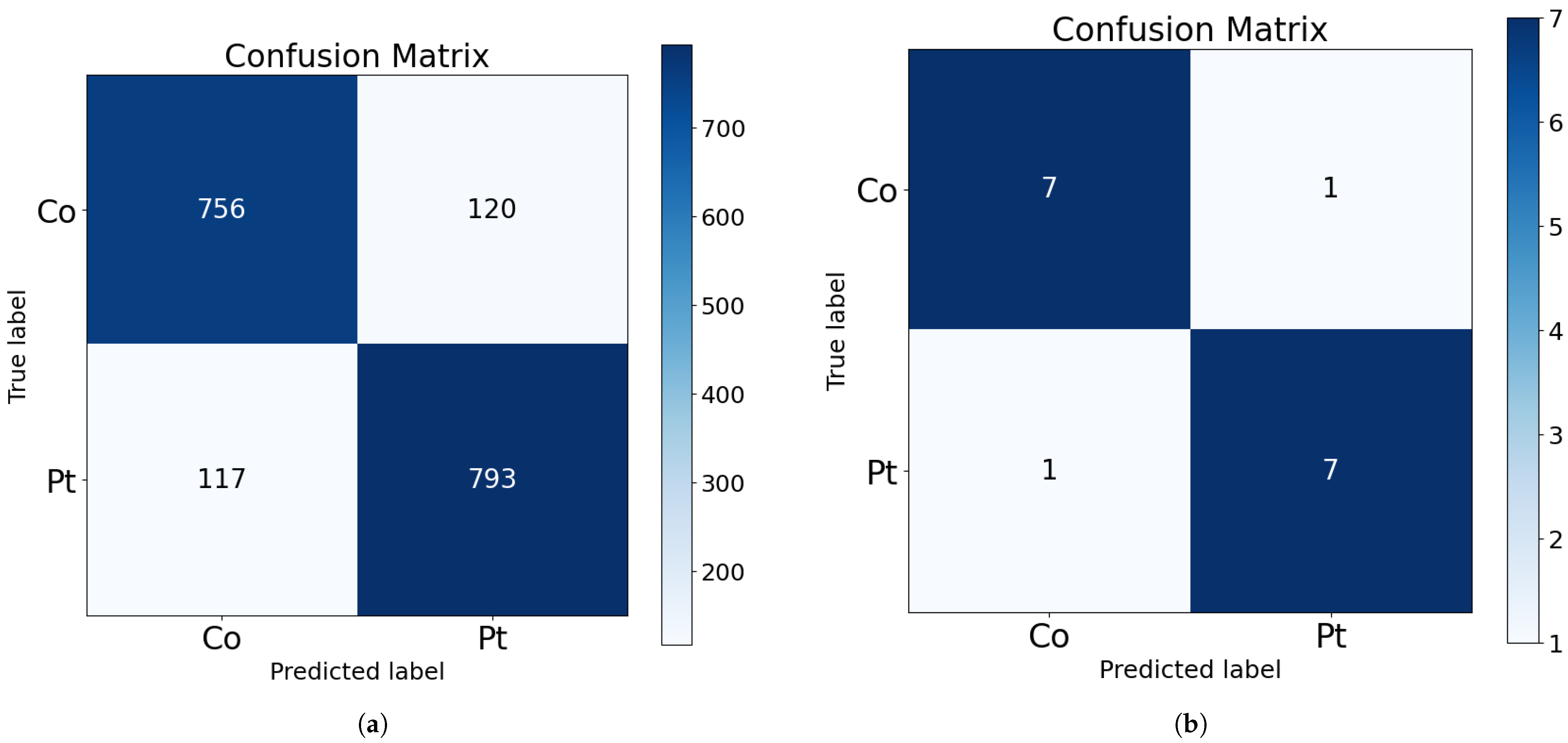
Their corresponding confusion matrices are shown in Figure 2. As shown in the bottom part of the figure, only one subject from each class is misclassified in the test subset. This corresponds to approximately 100 misclassified samples from each class (as visible in the upper part of the figure).

The confusion matrix illustrated in Figure 2b demonstrates an improved true positive rate and a more acceptable balance of false positives, in percentage terms, when compared to the results of the classification of individual samples. This outcome is more favorable for the use of the model as a diagnostic and screening tool.

Finally,

Table 5. Cross validation results.

	F1	F2	F3	F4	F5	F6	AVG	SD
Subjects
Acc. (Tr. subset)	0.93	0.94	0.95	0.95	0.94	0.93	0.94	0.01
Acc. (Test fold)	0.78	0.88	0.91	0.82	0.87	0.86	0.85	0.05
Rec. (Tr. subset)	0.98	0.99	0.99	0.99	0.99	0.99	0.99	0.00
Rec. (Test fold)	0.77	0.89	0.90	0.85	0.89	0.90	0.87	0.05
Subjects
Acc. (Tr. subset)	0.96	0.97	0.97	0.97	0.97	0.94	0.96	0.01
Acc. (Test fold)	0.81	0.87	0.94	0.87	0.87	0.81	0.86	0.05
Rec. (Tr. subset)	0.98	1	1	1	1	1	0.99	0.01
Rec. (Test fold)	0.81	0.94	0.97	0.90	0.81	0.90	0.89	0.06

presents the results obtained with the selected architecture using K-fold cross-validation with K = 6. For the case of sample classification (upper part of the table), the results obtained on the training set were very high for all the considered dataset combinations. The accuracy results exceeded 93% for all training subsets. Furthermore, when models were trained focusing on the recall metric, values above 98% were achieved for all training subsets, which is promising, suggesting the classifier’s potential as a screening tool.

For the results of each fold on the test subset, a decrease in performance values was observed, similar to those seen in the initial phase of this study. This suggests a dependency on the specific data used for training and a tendency to overfit to specific training characteristics. However, there is a significant variation in performance across specific folds, such as the first fold, suggesting that certain subjects may not exhibit the common gait characteristics prevalent in the rest of the dataset.

As previously done, performance metrics were extracted by classifying subjects based on all samples available for each individual. The results are shown in Table 5 (bottom part). With few exceptions, the results obtained demonstrated improvements compared to the classification of individual samples.

The best result was obtained with fold 3, achieving more than 90% accuracy for the classification of samples and more than 93% precision for the classification of subjects. The average results obtained for the final test of the best candidate were approximately 85% accuracy and nearly 87% recall for the test subset when working with samples. For the case of subject classification, the average results were over 86% accuracy and nearly 100% recall for the test subset.

Regarding the worst results obtained after cross-validation tests, these were observed with fold 1. For the case of sample classification, an accuracy of 78% and a recall of 77% were obtained for the test subset. And, for the case of classification of subjects, an accuracy and a recall of 81% were obtained. Thus, this implies a standard deviation of approximately 5% for samples and subjects, which is a relatively low value and acceptable for a diagnostic aid system.

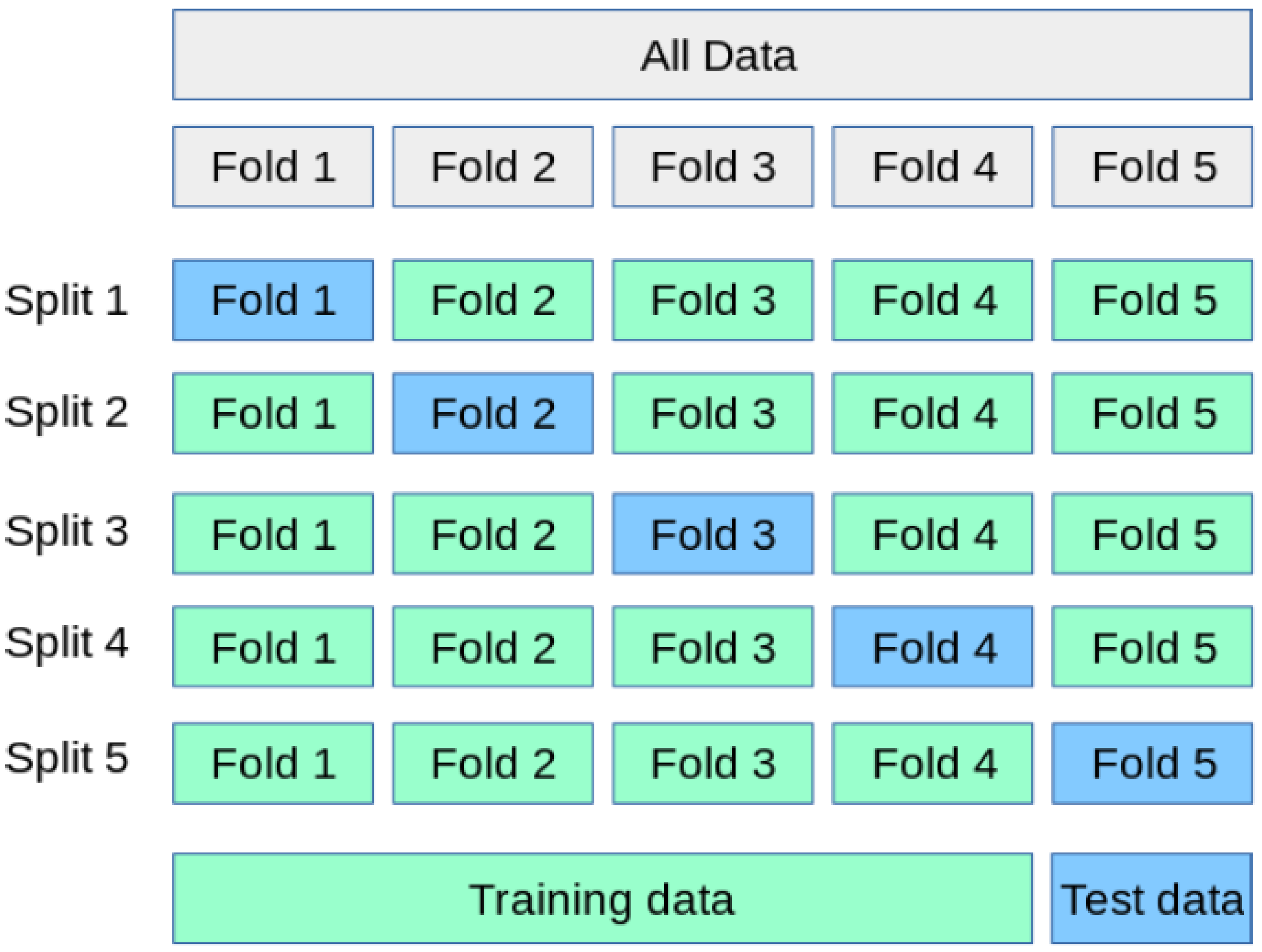
It is important to highlight that the variability observed in the K-fold cross-validation results can be attributed to the data partitioning strategy. To prevent data leakage, K-fold partitions were created at the subject level rather than the sample level. This implies that each validation fold could contain a set of subjects with gait patterns significantly different from those in the training set, which, in turn, introduces fluctuations in performance metrics across different folds. Despite these variations, the classifier’s accuracy never dropped below 78%, underscoring the overall robustness of the approach. Nevertheless, we acknowledge that to ensure greater stability and generalizability in real-world deployment scenarios, the use of larger and more balanced datasets will be required in future work.

In general, the results indicate that patients with Parkinson’s symptoms exhibit a very characteristic walking pattern. While this pattern may not be easily detectable in all patients, a system based on artificial intelligence techniques has proven useful in these circumstances, as, when pooling the correctly classified subjects from the training, validation, and test subsets, the combined accuracy is well over 95%.

Finally, to compare the results of this work with those obtained in previous studies, a bibliographic search was conducted for journal articles published in the last 10 years that utilized the same dataset as this study. The search identified a total of three articles with generally favorable results, and a summary of all of them is summarized in

Table 6. Comparison with other works.

Study	Algorithm	Complexity	Assessment	Accuracy	Recall
[20]	LBP + MLP	Unknown	Hold Out	0.889	0.889
[21]	RNN (LSTM) + CNN	$2\ast R_{LSTM}L+2\ast CL+2\ast PL+1\ast DL$	Hold Out	n/a	0.9861
[22]	FE + LWRF	Unknown	Cross-val (K = 10)	0.99 (max.)	0.978 (max.)
[23]	8 ∗ 1D-Convnet	$8\ast (4\ast CL+2\ast PL+1\ast DL)+2\ast DL$	Cross-val (K = 5)	0.987 ± 0.023	0.981 ± 0.033
[32]	CNN	$1\ast CL+1\ast PL+4\ast (2\ast CL+2\ast PL)+2\ast DL$	Train + Val. + Test	0.955 ± 0.003	n/a
Proposed-Average	RNN (GRU)	$1\ast R_{GRU}L$	Cross-val (K = 6)	0.86 ± 0.05	0.89 ± 0.06
Proposed Best	RNN (GRU)	$1\ast R_{GRU}L$	Cross-val (K = 6)	0.94 ± 0.05	0.97 ± 0.06

LBP: Local Binary Patterns; LSTM: Long-Short-Term Memory; R _$LSTM$L: LSTM layer; R_$GRU$L: GRU layer; MLP: Multi-Layer Perceptron; GRU: Gated-Recurrent Unit; DL: Dense layer; PL: Polling layer; RNN: Recurrent Neural Network; CNN: Convolutional Neural Network; CL: Convolutional layer; FE: Feature Extraction; LWRF: Locally Weigthed Random.

.

In this table, to facilitate comparison, the average and the best results obtained in this work were included as the last two rows.

Analysis of the results from previous studies indicates that high accuracy results were achieved in all of them. This means that the dataset is highly representative and that the patterns of Parkinson’s patients are readily detectable.

However, in these previous studies, different techniques were employed to classify and validate the results, which underscores the unique value of the present work.

Given the similar accuracy in many of the works, execution time, a common performance metric for hardware systems, could be used for comparison, although none of the identified papers present such a study. Therefore, a thorough comparison would ideally involve implementing the algorithms and classifiers from the previous papers on the same device to measure, under identical hardware constraints, the execution times of each of the models.

However, previous works often do not (in most cases) provide a detailed description of their classifiers (only a theoretical and/or graphical description), making their practical implementation challenging.

For this purpose, we refer to a previous study conducted by some of the current authors, which provides a comparison of execution times between classifiers based on classical neural networks and recurrent neural networks [31]. These experiments were performed under the same hardware constraints (processor, memory, gpu), the same software constraints (programming language, libraries) and the same data constraints (dataset, subset split, and preprocessing).

In this work, average running (classification) times were presented for artificial neural networks with 1 and 2 hidden layers, as well as for recurrent neural networks of LSTM and GRU types (with one and two layers each). The results of the execution times are summarized in

Table 7. Final results obtained from work [31].

Classifier	Avr. Exec. Time (s)	STD (s)
LSTM (1 layer)	2.34 × ${10}^{-2}$	4.13 × ${10}^{-4}$
GRU (1 layer)	2.78 × ${10}^{-2}$	3.17 × ${10}^{-4}$
LSTM (2 layers)	4.67 × ${10}^{-2}$	7.45 × ${10}^{-4}$
GRU (2 layers)	5.52 × ${10}^{-2}$	7.96 × ${10}^{-4}$
ANN (1 layer)	3.38 × ${10}^{-3}$	1.91 × ${10}^{-4}$
ANN (2 layers)	4.79 × ${10}^{-3}$	3.72 × ${10}^{-4}$

.

From Table 7, it is observed that a classification algorithm with one GRU layer takes approximately 10 times longer than a classical ANN with one hidden layer (a factor also applicable to a single LSTM layer), whereas two LSTM layers take 15 times longer. Thus, assuming a worst-case scenario for this study, we hypothesize that a fully connected layer has an execution time of T and, based on Table 7, one GRU layer has an execution time of $10T$, and two LSTM layers have an execution time of $15T$. While more complex processing layers (such as convolutional layers and pooling layers), their execution time will be longer than T, but we will consider the most conservative case for our analysis and assume that all non-recurrent layers will have an execution time of T.

Taking these assumptions into account,

Table 8. Hypothetical execution times, based on the study [31].

Study	Exec. Time (T)	Comparative
[20]	–	–
[21]	20T	200%
[22]	–	–
[23]	58T	580%
[32]	20T	200%
Proposed (2023)	10T	100%

summarizes the hypothetical execution times for each work under the same conditions.

From the first article [20], the comparison is complex, as the number of dense layers included in its ANN is not detailed in the manuscript. Furthermore, it is not possible to estimate the complexity of the preceding LBP feature extraction layer. All that can be seen in the paper is the presence of 4 processing blocks (one of which is the ANN network of unknown complexity). Even so, this work presents several unspecified unknowns: since it does not use cross-validation, it is unclear how many training runs were conducted to find a division between training, validation, and test that provides the shown results; additionally, the division percentages of the subsets are not indicated (nor whether a validation set was used); furthermore, it is not specified whether the accuracy results presented are from the test set or the total dataset (which would inflate the actual classification results of the system); and finally, the best accuracy results obtained do not surpass the best results achieved in our work.

Continuing with the work by [21], in addition to the issue of not using cross-validation, this work lacks reported accuracy results (only recall is provided). Considering this metric, the results are similar to ours. However, comparing the complexity of the classifier system as indicated in Table 8, the optimistic estimate indicates a complexity of 200% compared to our classifier.

Regarding the work of [22], the accuracy and recall results are notably high; however, only the best outcomes obtained with a K = 10-fold cross-validation are illustrated, and no information is provided on the distribution of the data, which limits comparative analysis. In terms of computational complexity, again due to the nature of the implementation, comparison becomes complex. Random Forest can be implemented with high efficiency, even on embedded systems. However, for improved precision, the proposed model adjusts the information obtained from each step based on certain neighbors within the dataset. This requires the dataset to be accessible during execution, which may be unfeasible for embedded systems due to resource limitations. Furthermore, feature extraction involves computationally expensive calculations.

The work of [23] presents results that surpass ours regarding accuracy and recall. Similarly, the validation mechanism, utilizing cross-validation, is highly similar to ours. On the other hand, the best model presented in [32] also achieves superior precision, in this case without employing cross-validation. However, if we compare these works in terms of execution time, the optimistic forecast made in Table 8 indicates that they exhibit execution times approaching 600% and 200%, respectively, relative to our work.

These results show that our classifier achieves nearly the best classification results while maintaining a leading position in computational efficiency, as for comparable results, we achieve a substantial improvement in execution time. This aspect is not critical when utilizing high-capacity computing equipment (such as a hospital computer), but it is crucial for integrating the classifier into a wearable device.

To further support the feasibility of deploying our model in wearable devices, we conducted a simulation using the X-Cube-AI framework provided by STMicroelectronics. The analysis was configured for an STM32F411RE microcontroller (Cortex-M4), and the results confirmed that the proposed GRU-based classifier fits within the memory and computational constraints of the device. Specifically, the model size was estimated at approximately 196 KB, which fits comfortably within the available flash memory. The estimated inference time was around 120 milliseconds, a plausible response time for continuous monitoring scenarios, where new samples are acquired during each inference cycle. While a direct comparison to all state-of-the-art models on this specific hardware was infeasible due to various constraints, including the impracticality of re-implementing every architecture and limitations of the deployment toolchain, these results are consistent with those reported in a previous study [17], in which a similar GRU-based architecture was successfully deployed on a real STM32 embedded system. The reported memory footprint and inference speed suggest that our solution significantly reduces the computational overhead compared to larger, multi-layer architectures or those reliant on complex feature engineering, making it well-suited for resource-constrained wearable applications. These findings reinforce the potential of our approach for real-time execution on low-power platforms.

Furthermore, based on a comparative assessment of model complexity, we estimate that alternative architectures proposed in the literature—particularly those with 2× to 6× higher computational demands—would likely require more capable embedded systems with increased memory and processing speed to achieve real-time inference. While such systems may deliver slightly higher classification accuracy, they would also entail increased energy consumption and hardware cost. These trade-offs are critical when selecting an appropriate model for deployment in wearable diagnostic applications, where efficiency and portability are essential. This aspect has previously been addressed in previous work by this research group, such as [33], demonstrating that low computational cost classification algorithms can be run in real time on embedded systems with low computational resources.

Limitations and Future Work

Despite the promising results presented in this study, several limitations should be acknowledged. Firstly, we did not carry out a systematic analysis of misclassified instances; therefore, the specific gait patterns leading to false positives and false negatives remain unclear. Analyzing these misclassifications could reveal valuable insights into model weaknesses and guide improvements. Secondly, our evaluation relied exclusively on the “Gait in Parkinson’s Disease” dataset. Although this dataset is comprehensive in terms of sensor coverage, its subject pool is limited and unevenly distributed between disease severity levels: certain stages are represented by only one participant. Because our K-fold splits are performed at the subject level to avoid data leakage, folds that isolate these unique participants in the test set can exhibit lower accuracy, reflecting the model’s difficulty in generalising to under-represented gait patterns. Future studies should incorporate larger and better balanced cohorts—ideally with explicit metadata on Parkinson’s severity—to mitigate this issue and improve generalizability.

Furthermore, while the dataset contains rich clinical metadata such as Hoehn & Yahr stage, medication status, and comorbidities, these variables were not utilized in the current study. This was a deliberate choice to align with our envisioned wearable implementation, which relies solely on plantar-pressure signals in everyday use. Consequently, omitting these variables limits our ability to assess how model performance may vary with disease severity or medication state. However, we acknowledge that leveraging such information holds significant potential for future extensions aiming to improve accuracy or enable more personalized models.

Moreover, further research could explore the integration of multimodal sensor input beyond plantar pressure sensors, potentially enhancing classification accuracy and robustness.

The present study primarily focuses on demonstrating the technical feasibility that plantar-pressure data alone can support reliable classification of Parkinson’s gait patterns; however, it is not intended to replace or replicate comprehensive neurologist evaluation. In practice, a wearable implementation would primarily operate as an early-screening or continuous-monitoring aid. When the algorithm detects a sustained pattern suggestive of Parkinson’s disease, the device would notify both the user and a healthcare professional, prompting a formal clinical examination (e.g., UPDRS scoring) rather than delivering a stand-alone diagnosis. Such integration could accelerate referral for specialist assessment and facilitate objective, longitudinal tracking of gait changes between clinic visits, thereby complementing neurologist judgement rather than competing with it.

It is also crucial to acknowledge the practical consequences of misclassifications. While our best model achieves solid subject-level performance (accuracy ≈ 0.88, precision ≈ 0.94, recall ≈ 0.88; see Table 4), any misclassification could have significant implications. False negatives are of particular concern because an undetected patient may miss out on timely intervention, which could lead to worsening disease progression. False positives, while medically less dangerous, can still impose psychological stress and lead to unnecessary follow-up testing. Therefore, this classifier is intended strictly as a screening aid and must always be followed by a comprehensive clinical evaluation. In any real-world deployment, results would be reviewed by a qualified clinician before any diagnosis is communicated, ensuring a human-in-the-loop safeguard and adherence to ethical guidelines for diagnostic support systems. Prospective validation under appropriate ethical approval will be an essential next step.

Finally, although we conducted detailed simulations confirming the feasibility of deployment on embedded hardware, we did not perform a full hardware implementation on an actual wearable device. Such an implementation and validation in real-world conditions represents an essential next step. It would allow us to observe the behavior of the models when integrated and executed over extended periods on embedded platforms designed for wearable applications. This would help confirm whether the performance metrics observed in this study remain stable in practice and would also enable the measurement of actual power consumption and device autonomy, which are critical parameters for real-world usability. A full treatment of other real-world engineering aspects, such as comprehensive power consumption analysis, sensor drift mitigation, on-device inference latency optimization, and robust handling of motion artifacts, lies beyond the scope of this initial study, but will be thoroughly addressed during the forthcoming hardware-integration and real-world validation phases.

5. Conclusions

There is no standard diagnostic mechanism for Parkinson’s disease. However, the literature suggests the utility of physical activity monitoring techniques. Notably, the dataset collected by [29], which contains biomechanical gait data from patients with the disease.

Building upon this, the present work develops a classifier system that distinguishes between Parkinson’s disease patients and healthy controls using Deep Learning techniques, specifically Recurrent Neural Networks.

To obtain the best classifier, an optimization process was conducted in two phases: commencing with a grid search combining various hyperparameter configurations for 1- and 2-layer GRU and LSTM architectures; Subsequently, the best candidate, identified by its accuracy results, was selected and subjected to additional cross-validation tests to assess the classifier’s final performance. The final classifier achieves an accuracy result of up to 91% (average ± SD: 85 ± 5%) for individual samples and up to 93.75% (average ± SD: 86 ± 5%) for subject-level classification.

These results are detailed and compared against the most prominent recent studies utilizing this same dataset.

This comparison highlights aspects where this work outperforms almost all previous studies. However, this work does not achieve accuracy as high as that reported in the studies by [23] (4 percentage points lower) and [22] (1 percentage point lower); but the designed classifier system is nearly six times and two times more computationally efficient, respectively, in terms of computational cost. This highlights a significant future direction for integrating this classifier algorithm into embedded systems, an aspect challenging for previous studies given their higher computational requirements.

Thus, a remarkable and novel aspect of this work is the demonstration that Parkinson’s disease can be detected by gait patterns using computationally efficient classifier algorithms; consequently, this classification could be performed in real time using a wearable device. However, it is crucial to reiterate that this classifier is intended strictly as a screening and continuous-monitoring aid, designed to complement, rather than replace, comprehensive clinical evaluations by neurologists. While simulations confirm the computational feasibility for deployment, future work will focus on full hardware implementation and real-world validation, addressing critical engineering aspects such as power consumption, sensor drift, on-device inference latency, and robust handling of motion artifacts. This will also include prospective validation against clinical assessments under appropriate ethical guidelines to further solidify its role in practical diagnostic pathways and to account for limitations such as dataset distribution and the non-utilization of all available clinical metadata.

References

1. World Health Organization. Parkinson Disease: A Public Health Approach: Technical Brief; World Health Organization: Geneva, Switzerland, 2022. [Google Scholar]
2. Tysnes, O.B.; Storstein, A. Epidemiology of Parkinson’s disease. J. Neural Transm. 2017, 124, 901–905. [Google Scholar] [PubMed]
3. Tansey, M.G.; Goldberg, M.S. Neuroinflammation in Parkinson’s disease: Its role in neuronal death and implications for therapeutic intervention. Neurobiol. Dis. 2010, 37, 510–518. [Google Scholar] [PubMed]
4. Savitt, J.M.; Dawson, V.L.; Dawson, T.M. Diagnosis and treatment of Parkinson disease: Molecules to medicine. J. Clin. Investig. 2006, 116, 1744–1754. [Google Scholar] [PubMed]
5. Tolosa, E.; Gaig, C.; Santamaría, J.; Compta, Y. Diagnosis and the premotor phase of Parkinson disease. Neurology 2009, 72, S12–S20. [Google Scholar]
6. Isroilovich, A.E.; Jumanazarovich, M.R.; Muxsinovna, K.K.; Askarovhch, M.B.; Yunusovuch, N.O. The Role and Importance of Gliah Neurotrophical Factors in Early Diagnosis of Parkinson Disease. Tex. J. Med. Sci. 2022, 5, 1–6. [Google Scholar]
7. Etoom, M. Therapeutic interventions for Pisa syndrome in idiopathic Parkinson’s disease: A scoping systematic review. Disabil. Rehabil. 2020, 42, 3534–3542. [Google Scholar] [CrossRef]
8. Armstrong, M.J.; Okun, M.S. Diagnosis and treatment of Parkinson disease: A review. JAMA 2020, 323, 548–560. [Google Scholar]
9. Salat, D.; Noyce, A.J.; Schrag, A.; Tolosa, E. Challenges of modifying disease progression in prediagnostic Parkinson’s disease. Lancet Neurol. 2016, 15, 637–648. [Google Scholar]
10. Pires, A.O.; Teixeira, F.G.; Mendes-Pinheiro, B.; Serra, S.C.; Sousa, N.; Salgado, A.J. Old and new challenges in Parkinson’s disease therapeutics. Prog. Neurobiol. 2017, 156, 69–89. [Google Scholar]
11. Espay, A.J.; Bonato, P.; Nahab, F.B.; Maetzler, W.; Dean, J.M.; Klucken, J.; Eskofier, B.M.; Merola, A.; Horak, F.; Lang, A.E.; et al. Technology in Parkinsonś disease: Challenges and opportunities. Mov. Disord. 2016, 31, 1272–1282. [Google Scholar]
12. Civit-Masot, J.; Bañuls-Beaterio, A.; Domínguez-Morales, M.; Rivas-Perez, M.; Muñoz-Saavedra, L.; Corral, J.M.R. Non-small cell lung cancer diagnosis aid with histopathological images using Explainable Deep Learning techniques. Comput. Methods Programs Biomed. 2022, 226, 107108. [Google Scholar]
13. Al Jowair, H.; Alsulaiman, M.; Muhammad, G. Multi parallel U-net encoder network for effective polyp image segmentation. Image Vis. Comput. 2023, 137, 104767. [Google Scholar]
14. Dominguez-Morales, J.P.; Jimenez-Fernanez, A.F.; Dominguez-Morales, M.J.; Jimenez-Moreno, G. Deep neural networks for the recognition and classification of heart murmurs using neuromorphic auditory sensors. IEEE Trans. Biomed. Circuits Syst. 2017, 12, 24–34. [Google Scholar] [PubMed]
15. Muñoz-Saavedra, L.; Luna-Perejón, F.; Civit-Masot, J.; Miró-Amarante, L.; Civit, A.; Domínguez-Morales, M. Affective state assistant for helping users with cognition disabilities using neural networks. Electronics 2020, 9, 1843. [Google Scholar] [CrossRef]
16. Kabir, M.M.; Shin, J.; Mridha, M.F. Secure Your Steps: A Class-Based Ensemble Framework for Real-Time Fall Detection using Deep Neural Networks. IEEE Access 2023, 11, 64097–64113. [Google Scholar]
17. Luna-Perejón, F.; Domínguez-Morales, M.J.; Civit-Balcells, A. Wearable fall detector using recurrent neural networks. Sensors 2019, 19, 4885. [Google Scholar] [CrossRef]
18. Kumar, A.K.; Ritam, M.; Han, L.; Guo, S.; Chandra, R. Deep learning for predicting respiratory rate from biosignals. Comput. Biol. Med. 2022, 144, 105338. [Google Scholar]
19. Abbasi, Q.H.; Heidari, H.; Alomainy, A. Wearable wireless devices. Appl. Sci. 2019, 9, 2643. [Google Scholar]
20. Ertuğrul, Ö.F.; Kaya, Y.; Tekin, R.; Almalı, M.N. Detection of Parkinson’s disease by shifted one dimensional local binary patterns from gait. Expert Syst. Appl. 2016, 56, 156–163. [Google Scholar]
21. Zhao, A.; Qi, L.; Li, J.; Dong, J.; Yu, H. A hybrid spatio-temporal model for detection and severity rating of Parkinson’s disease from gait data. Neurocomputing 2018, 315, 1–8. [Google Scholar]
22. Aşuroğlu, T.; Açıcı, K.; Erdaş, Ç.B.; Toprak, M.K.; Erdem, H.; Oğul, H. Parkinson’s disease monitoring from gait analysis via foot-worn sensors. Biocybern. Biomed. Eng. 2018, 38, 760–772. [Google Scholar]
23. El Maachi, I.; Bilodeau, G.A.; Bouachir, W. Deep 1D-Convnet for accurate Parkinson disease detection and severity prediction from gait. Expert Syst. Appl. 2020, 143, 113075. [Google Scholar]
24. Alkhatib, R.; Diab, M.O.; Corbier, C.; El Badaoui, M. Machine learning algorithm for gait analysis and classification on early detection of Parkinson. IEEE Sens. Lett. 2020, 4, 1–4. [Google Scholar]
25. Bengio, Y.; Simard, P.; Frasconi, P. Learning long-term dependencies with gradient descent is difficult. IEEE Trans. Neural Netw. 1994, 5, 157–166. [Google Scholar]
26. Hochreiter, S. The vanishing gradient problem during learning recurrent neural nets and problem solutions. Int. J. Uncertain. Fuzziness Knowl. Based Syst. 1998, 6, 107–116. [Google Scholar]
27. Hochreiter, S.; Schmidhuber, J. Long short-term memory. Neural Comput. 1997, 9, 1735–1780. [Google Scholar]
28. Cho, K.; Van Merriënboer, B.; Bahdanau, D.; Bengio, Y. On the properties of neural machine translation: Encoder-decoder approaches. arXiv 2014, arXiv:1409.1259. [Google Scholar]
29. Goldberger, A.L.; Amaral, L.A.; Glass, L.; Hausdorff, J.M.; Ivanov, P.C.; Mark, R.G.; Mietus, J.E.; Moody, G.B.; Peng, C.K.; Stanley, H.E. PhysioBank, PhysioToolkit, and PhysioNet: Components of a new research resource for complex physiologic signals. Circulation 2000, 101, e215–e220. [Google Scholar]
30. Sokolova, M.; Lapalme, G. A systematic analysis of performance measures for classification tasks. Inf. Process. Manag. 2009, 45, 427–437. [Google Scholar]
31. Escobar-Linero, E.; Luna-Perejon, F.; Munoz-Saavedra, L.; Sevillano, J.L.; Domínguez-Morales, M. On the feature extraction process in machine learning. An experimental study about guided versus non-guided process in falling detection systems. Eng. Appl. Artif. Intell. 2022, 114, 105170. [Google Scholar]
32. Alharthi, A.S.; Casson, A.J.; Ozanyan, K.B. Gait spatiotemporal signal analysis for Parkinson’s disease detection and severity rating. IEEE Sens. J. 2020, 21, 1838–1848. [Google Scholar]
33. Luna-Perejón, F.; Domínguez-Morales, M.; Gutiérrez-Galán, D.; Civit-Balcells, A. Low-power embedded system for gait classification using neural networks. J. Low Power Electron. Appl. 2020, 10, 14. [Google Scholar]
Figure 1. K-fold cross validation. Representation with K = 5.
Bdcc 09 00183 g001
Figure 2. Confusion Matrices. (a) Results using test samples. (b) Results classifying subjects in test subset. ‘Co’: Control group, ‘Pt’: Patients with Parkinson.
Bdcc 09 00183 g002