Abstract
Human visual attention is influenced by multiple factors, including visual, auditory, and facial cues. While integrating auditory and visual information enhances prediction accuracy, many existing models rely solely on visual-temporal data. Inspired by cognitive studies, we propose a computational model that combines spatial, temporal, face (low-level and high-level visual cues), and auditory saliency to predict visual attention more effectively. Our approach processes video frames to generate spatial, temporal, and face saliency maps, while an audio branch localizes sound-producing objects. These maps are then integrated to form the final audio-visual saliency map. Experimental results on the audio-visual dataset demonstrate that our model outperforms state-of-the-art image and video saliency models and the basic model and aligns more closely with behavioral and eye-tracking data. Additionally, ablation studies highlight the contribution of each information source to the final prediction.
1. Introduction
The amount of information obtained through human vision far exceeds what the central nervous system can process [1]. However, the human ability to focus on important and salient information enables effective management of vast visual input. This capability of the human visual system (HVS) is known as visual attention [2]. Modeling and predicting visual attention is critical across various applications, as it allows machines to replicate human focus and identify the most relevant elements.
Saliency maps are fundamental to computational attention modeling, offering a structured framework for identifying perceptually relevant regions based on visual, auditory, or multimodal cues. In static images, they capture spatial features, while in dynamic scenes, temporal saliency maps incorporate motion patterns to refine attentional predictions [1]. Audio saliency maps, in turn, detect significant sound events in audio-visual content. Integrating these saliency types enhances the predictive accuracy of attention models in multimodal settings, supporting a comprehensive understanding of human perception [3].
Over the recent years, numerous models for predicting visual saliency have been proposed, demonstrating substantial promise [1,4]. These models rely solely on visual cues to identify elements that stand out from their surroundings. However, the world consistently presents multimodal information [3], perceived through senses such as vision, hearing, smell, touch, and taste. These sensory modalities interact, integrating and directing human attention. Thus, visual attention is not isolated; it can be influenced by other senses [5]. Behavioral experiments, neuroimaging studies, and everyday experiences provide strong evidence that human behavior is shaped by the integration of multimodal sensory information [6].
In addition to vision, hearing is the second-largest source of sensory input. Coutrot et al. [7] discovered that sound can impact visual attention, and audiences watching videos, both with and without sound, tend to focus on different locations. Song et al. [8] observed that the impact of sound varies by content type (e.g., music, action sounds, human voice), with the human voice having the most significant effect. In [9], the authors demonstrated that sound’s influence depends on its compatibility with visual signals. When the sound source is not the most visually significant object, attention is partially drawn to it. For example, in conversations, subjects focus more on the speaker. With sound, the source influences attention; without sound, attention relies on visual cues. Thus, visual information alone cannot predict where humans will look, as shown in Figure 1 [9]. In Figure 1, one object stands out visually, but another is salient auditorily, leading viewers to look at different locations depending on the presence of sound. For further details on methods examining the impact of sound on visual attention, readers may refer to [7,8,9].
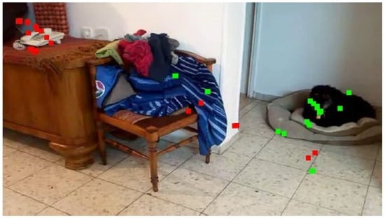
Figure 1.
The red squares represent fixations recorded in both audio and visual conditions, and the green squares represent points recorded in visual conditions only [9].
Videos are typically accompanied by audio. Despite established evidence of the interplay between auditory and visual signals and their combined influence on visual attention [10], most video saliency models focus primarily on low-level visual cues, overlooking high-level and auditory information. Low-level cues include color, orientation, brightness, corners, and edges, while high-level cues involve semantic content, facial recognition, and central bias. Building on these findings, we propose an audio-visual saliency model that integrates auditory, low-level, and high-level visual information to predict saliency in videos, achieving better alignment with behavioral and eye-tracking data. Experimental results on audio-visual attention databases show that our model outperforms both audio-visual and state-of-the-art static and dynamic saliency models. Ablation studies further reveal insights into the impact of audio, visual, and motion stimuli on predicting visual attention in videos with audio. Our contributions are as follows:
- Modeling visual attention by integrating low-level and high-level visual cues, motion, and auditory information.
- Applying implicit memory principles to merge the generated maps and create the final audio-visual saliency map.
- Assessing the significance of each information source in the proposed model through an ablation study.
Outline: Section 2 discusses background concepts of visual attention in static and dynamic environments, as well as multimodal visual attention models. In Section 3, we describe our audio-visual attention model. We analyze the experimental results in Section 4 and provide a summary and conclusion for this paper in Section 5.
2. Literature Review
Visual attention has long been a critical area of research in psychology, image processing, and computer vision. In this section, we review the literature from three perspectives: visual attention in static environments, dynamic environments, and multimodal visual attention.
2.1. Visual Attention in Static Environments
Many attention models are based on Treisman and Gelade’s Feature Integration Theory [11], which explains the integration of visual features in human attention mechanisms during visual search. Koch and Ullman [12] introduced a feed-forward model incorporating a saliency map to highlight prominent regions in a scene. This foundation led to Itti et al.’s saliency-based attention model [13], which consists of three stages: (1) constructing a Gaussian pyramid where static features (color, intensity, and orientation) are extracted, (2) generating center-surround feature maps and normalizing them into conspicuity maps, and (3) computing a linear combination to produce the final saliency map. Harel et al. [14] introduced the graph-based visual saliency (GBVS) model, which constructs a fully connected graph over feature maps extracted similarly to the Itti model [13]. Nodes represent spatial locations, while edge weights, inspired by Markov chains [15], are assigned based on spatial proximity and feature dissimilarity. Hou and Zhang [16] proposed the spectral residual saliency model, which utilizes the Fourier transform to extract the log spectrum of an image and emphasizes residual components corresponding to salient regions. The Bayesian saliency model [17], based on natural statistics, enhances prediction accuracy by learning feature distributions over time. These models primarily focus on saliency detection in static scenes using spatial features.
Figure 2 presents the saliency maps computed by these models for a frame from the multimedia dataset [18].
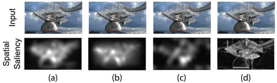
Figure 2.
Saliency maps produced by the proposed models in the static visual attention segment: (a) Itti and Koch, (b) GBVS, (c) Hou and Zhang, (d) SUN.
2.2. Visual Attention in Dynamic Environments
In dynamic environments, motion information plays a pivotal role [19]. Although saliency detection and object segmentation have distinct objectives, they are closely interrelated, as many segmentation models leverage saliency cues. Fang et al. [20] proposed a video saliency model integrating spatial-temporal information with statistical uncertainty. The model leverages proximity theory, Gestalt principles, and background motion variations to enhance dynamic saliency detection. Wang et al. [21] improved stability by incorporating gradient flow and energy optimization. It constructs spatial-temporal maps to differentiate foreground from background, dynamically adjusting surrounding regions based on background distance. Liu et al. [22] utilized superpixel-based graphs for saliency estimation, refining results through shortest path algorithms. Rogalska and Napieralski [23] developed a model integrating global contrast, image center distance, human face detection, and motion for constructing saliency maps. Shabani et al. [24] proposed a bottom-up visual attention model that fuses multiple saliency maps via a gating network and combiner. Their approach leverages four established saliency models [13,14,16,25,26], along with skin detection and face localization. A deep learning-based mediation network adaptively integrates these maps, producing a final saliency map closely aligned with human visual attention. While these models emphasize saliency detection, Wang et al. [25,26] introduced a geodesic distance-based segmentation method, constructing spatio-temporal edge and optical flow maps. The final segmentation is refined through object skeleton abstraction. Although these models effectively capture motion-driven attention, they are limited to visual cues, neglecting audio influences. Figure 3 presents the saliency maps predicted in dynamic environments by these models using the ETMD dataset [27], which contains human-annotated Hollywood movie clips with complex semantics.
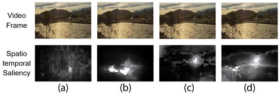
Figure 3.
Saliency maps generated in dynamic environments using the proposed models: (a) Fang et al. (2014) [20], (b) Wang et al. (2015) [21], (c) Liu et al. (2017) [22], (d) Wang et al. (2018) [26].
2.3. Multimodal Visual Attention
Fixation prediction models commonly incorporate low-level or high-level visual features to identify salient regions, with a primary focus on visual perception. While psychological studies have demonstrated the influence of sound on visual attention, these insights have yet to be widely integrated into computational models of visual attention. Although visual saliency is a well-established field, research on audio-visual saliency remains in its early stages [28,29]. Existing visual saliency models can be broadly categorized into two types: deep learning-based models and handcrafted models. Audio-visual saliency modeling faces significant challenges, including limited training datasets and performance bottlenecks in deep learning models due to overfitting [28,29]. To overcome these challenges, we propose a handcrafted computational model of audio-visual attention that does not require extensive training data, thereby enhancing generalizability and interpretability compared to data-driven approaches. A fundamental component of multimodal saliency modeling is audio signal processing. Mel-frequency Cepstral Coefficients (MFCCs) [30] have proven effective in capturing sound frequency characteristics and are commonly used in speech recognition and environmental sound analysis. We leverage MFCCs to integrate auditory signals with visual saliency models, improving multimodal attention prediction. Several studies have attempted to incorporate auditory cues into saliency prediction. Kaiser’s model [31], inspired by the Itti visual saliency model [13], converts auditory stimuli into a time–frequency representation, extracting intensity, temporal contrast, and frequency contrast to generate a saliency map. However, this model is limited to auditory processing and does not integrate visual cues. Izadinia et al. [32] introduced a model that identifies moving objects associated with sound by extracting audio and visual features and applying Canonical Correlation Analysis (CCA). CCA is a statistical technique used to identify linear correlations between two sets of multidimensional variables, making it useful in multimodal data fusion. However, CCA is limited to modeling linear dependencies and does not fully capture complex audio-visual interactions [33]. This model is based on the assumption that moving objects generate audible sounds and variations in movement are reflected in changes in the auditory signal. This model effectively links motion and auditory cues but lacks explicit consideration of static visual features that contribute to attention. Min et al. [32] extended this approach by computing spatial and temporal attention maps from video streams. The video is divided into spatial-temporal regions (STRs), and visual features for each STR are extracted. The audio signal is aligned with the video frames, and MFCCs with their first-order derivatives (MFCC-Ds) are computed to represent the audio. CCA is used to identify STRs with the highest correlation between visual and auditory features, resulting in an integrated audio-visual saliency map. However, this approach still relies on linear correlations, limiting its ability to model complex multimodal relationships.
To address these limitations, Min et al. [5] introduced the Multimodal Saliency (MMS) model, which enhanced audio-visual integration by incorporating Kernel Canonical Correlation Analysis (KCCA).
Unlike CCA, which captures only linear dependencies, KCCA uses kernel functions to map data into a higher-dimensional space, enabling the modeling of nonlinear relationships. This improvement boosts the accuracy of sound saliency localization. However, the MMS model has certain shortcomings:
- Performance in motion-heavy scenes: In highly dynamic environments, excessive background motion can interfere with sound localization, reducing accuracy.
- Lack of face saliency modeling as high-level visual features: Prior research [30] has shown that observers consistently focus on faces in images, even when instructed to focus on competing objects. This effect is particularly evident in scenes like conversations. The MMS model does not explicitly consider these features, leading to potential mispredictions in face-dominant scenes.
To overcome these challenges, we build upon the MMS model by integrating a more refined face saliency map and improving the fusion of spatial, temporal, and auditory cues. Our approach enhances fixation prediction, especially in conversational and highly dynamic scenarios where previous models struggle. The results demonstrate superior performance in several video scene examples, as shown in Figure 4.
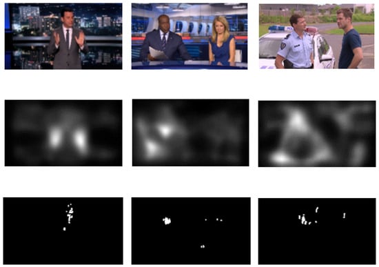
Figure 4.
Result of MMS model. From top to bottom: main video frame, MMS, and human eye fixation.
By addressing the limitations of previous methods and refining the integration of multimodal cues, our proposed model significantly advances audio-visual attention prediction.
3. Materials and Methods
The framework of the proposed model is illustrated in Figure 5. It comprises four streams: spatial saliency, face saliency, temporal saliency, and audio saliency. Spatial, temporal, and face saliency maps are derived from intra-frame and inter-frame information. Audio saliency is computed by using audio and video streams to localize moving-sounding objects. The visual and audio saliency maps are then fused to generate the final audio-visual saliency map.Table 1 provides a formal summary of the notations and symbols employed throughout this study.
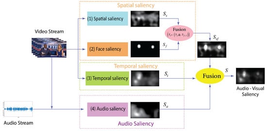
Figure 5.
Framework of our proposed model.

Table 1.
Notations and symbols.
3.1. Detection of Spatial Saliency
The human visual system does not directly translate retinal stimuli but rather interprets them through complex psychological inference based on past experiences [34]. Vision emerges from the dynamic interaction between the brain and visual input, necessitating that saliency detection models estimate brain responses to stimuli. Friston [35] unified multiple theories of brain function related to perception, action, and learning within the free-energy framework. According to this principle, the brain continuously refines its interpretation of visual stimuli by reducing uncertainty, guided by an internal generative model (IGM). This model plays a fundamental role in cognitive processes and aligns with key theories in both the biological and physical sciences. The free energy principle posits that the brain minimizes uncertainty and counteracts entropy to maintain a stable perceptual state. The discrepancy between external visual stimuli and the brain’s IGM creates a perceptual gap, leading to surprise, which in turn enhances attention and influences visual saliency [34]. Free energy best measures the difference between the input visual signal (I) and the sample inferred by the internal generative brain model (IGM), () [5]. This difference is linked to the surprise recognized by the brain and can therefore be utilized to identify visual saliency [36]. The Autoregressive (AR) model is considered an internal generative model (IGM) that can regenerate natural image structures using a simple yet powerful method. Each pixel is modeled as follows:
where denotes the pixel intensity at location i, is the vector of neighboring pixel values of , k is the number of neighbors (set to 8, as in [5]), is the vector of AR model coefficients, and is the prediction error. The coefficients w are optimized as follows:
The matrix Y encodes the neighborhood information of each pixel and denotes a local patch of the image centered at pixel x. The coefficients w are estimated using the least squares method as follows:
The AR model generates a predicted version of the input image I:
After estimating the predicted image through the AR model, the free energy is calculated:
where N is the total number of pixels, and is the likelihood of the given image according to the internal generative model. For simplicity, the second term (model cost) is often considered constant and is neglected. To compute the visual saliency map, the entropy of the error map is used:
This computation is performed across different color channels, and the entropy maps are filtered and normalized:
where g is a Gaussian filter used for noise reduction, is a normalization operator that scales the map values to the range [0, 1], and ∗ denotes the convolution operator. For further details, readers are referred to [34,35,36].
3.2. Detection of Face Saliency
Under natural viewing conditions, the human gaze typically fixates on image regions that capture attention. Specifically, faces consistently draw focus, as noted in previous studies [37]. Based on these findings, we use face saliency as an additional saliency map, employing the MTCNN deep learning-based face detection algorithm. Older face detection methods were often affected by factors such as head position, facial expressions, and lighting conditions, which impacted performance.
The MTCNN algorithm was developed for face detection and alignment, using a cascade of three convolutional neural networks. First, the image is resized multiple times to detect faces of varying sizes [38]. The first network (P-NET) scans the image to identify potential face regions. While it operates quickly, it has low accuracy and a high false positive rate. The second network (R-NET) refines these detections by removing incorrect areas, with more parameters and improved performance. The third network (O-NET) is more complex and slower, with additional parameters and layers, and further refines the accuracy by determining the presence of a face and precisely locating facial landmarks such as the eyes, nose, and mouth corners. Figure 6 [38] illustrates the output of the face detection algorithm.
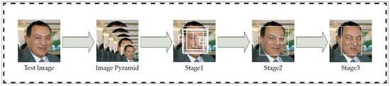
Figure 6.
MTCNN face detection algorithm performance [38].
3.3. Detection of Temporal Saliency
Motion information is a key cue for visual attention. Several techniques for extracting motion features are discussed in the literature, including optical flow [39], motion vectors [40], and frame differences [41]. In this paper, we adopt inter-frame differences, as proposed in the base model [5], to detect motion and use it as a measure of temporal saliency. This method is computationally efficient and effectively captures significant movements, enabling the detection of motion changes in the scene without high computational cost. Specifically, we calculate the intensity of each frame as described in Equation (8).
Let f denote the frame index, with , , and representing the color channels of frame f. The motion feature can be determined from the inter-frame difference, as indicated in Equation (9).
Let t be the frame latency parameter. In accordance with [5], we assign the value of 3 to t. Subsequently, following the application of the Gaussian filter to the motion feature, the temporal saliency is computed:
The frame index f is excluded for the sake of simplicity. Index t denotes temporal saliency, ∗ represents the convolution operator, and g signifies a local Gaussian filter.
3.4. Audio Saliency Detection
The proposed model targets scenes with high audio-visual correspondence, where sound originates from object movement. We localize the moving-sounding objects in these scenes by adopting the method outlined in the baseline model [5]. Figure 7 presents an image of the sound localization framework using this method. According to [5], we perform the following three steps to localize the sound.
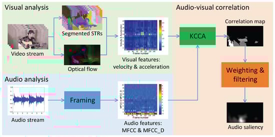
Figure 7.
Stages of audio saliency detection [5].
Step (1) Visual analysis: The process of visual analysis involves three stages. Dividing the entire video into a set of spatial-temporal areas (STRs), extracting visual features such as velocity and acceleration from forward and backward optical flow, and describing each STR using the extracted visual features. Figure 8 illustrates these stages for a sample video frame.
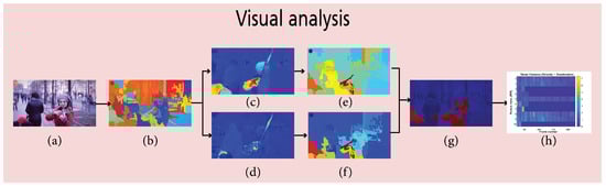
Figure 8.
Illustration of the visual analysis results corresponding to a sample frame from the input video. (a) Frame F, (b) STRs extracted from frame F, (c) velocity of F (), (d) acceleration of F (), (e) mean velocity magnitude for each STR, (f) mean acceleration magnitude for each STR, (g) STRs with the highest variance, and (h) visual features (velocity and acceleration).
From the adjacent frames, forward and backward optical flow is extracted to describe the local motion. Then, the characteristics of velocity and acceleration of each frame are calculated as follows:
denotes the forward optical flow, computed from frame to , while represents the backward optical flow from frame to . Subsequently, STRs are characterized by the average velocity and average acceleration of all their pixels.
To reduce the candidate STRs, the STRs exhibiting greater velocity over time and the STRs demonstrating higher acceleration over time are chosen based on their variances along the time axis, resulting in the creation of the V matrix (). Subsequently, we employ the V matrix to characterize the visual attributes of the entire video.
denotes the visual feature of STR . r represents the STR index, f denotes the frame number, and .
Step (2) Audio analysis: As shown in Figure 7, the analysis process begins by extracting acoustic features associated with the target object’s movement. The audio signal is assumed to primarily consist of sound produced by the moving object. Before feature extraction, a windowing technique segments the audio signal to align the number of audio frames with the video frames. Since audio is recorded at a much higher sampling rate than video, the signal is divided into overlapping time windows with a 50% overlap to ensure synchronization. This preserves frequency continuity and enables more accurate feature extraction. To further retain frequency characteristics, a Hamming window is applied during framing, with the frame length dynamically adjusted according to the sampling rate.
Following segmentation, extract MFCC features and MFCC-D features as the audio representation, and construct matrix A, where . Matrix A captures the audio characteristics corresponding to the video frames.
, represents an N-dimensional vector. It comprises MFCCs and MFCC-Ds, utilized to characterize the audio signal of the fth frame.
MFCC features capture essential spectral information from audio signals, such as speech or impulsive sounds, while MFCC-D features represent their temporal dynamics, including sudden or transient events. Although these features do not directly convey spatial information, their temporal patterns support synchronization with visual events. This enables the alignment of audio and visual streams across corresponding frames, improving the localization of the sound source. The feature matrix A, which reflects the intensity of these features over time, is essential for audio-visual correlation analysis.
Step (3) Audio-visual correlation: The audio-visual correlation process aims to identify STRs within a video that strongly correlate with accompanying audio signals. Traditional linear methods often fall short due to inherent differences between audio and visual feature spaces. To address this, the present study employs to project features into a high-dimensional space. This enables the discovery of complex intermodal relationships and facilitates the identification of STRs with strong cross-modal correlations, serving as key auditory sources or salient moving objects. These STRs ultimately contribute to constructing an audio saliency map.
In the first step, audio and visual features are mapped to the kernel space using a non-linear transformation . Similarity between data points in this space is defined by a symmetric, positive semi-definite kernel function. This study employs a Gaussian kernel, defined as follows:
Here, x and y represent feature vectors, is a parameter that controls the kernel width, and denotes the inner product.
The objective of is to find pairs of canonical vectors and that maximize the linear correlation between mapped visual features V and audio features A:
Here, , , and denote the cross-covariance matrix between the visual and audio modalities, the covariance matrix of the visual features, and the covariance matrix of the audio features, respectively. To express the optimization problem in the kernel space, the canonical vectors are reformulated as follows:
By substituting the expressions into Equation (16), the final form of the optimization problem is derived as follows:
In this formulation, and are the kernel Gram matrices for the visual and audio data, respectively. The parameter denotes the regularization coefficient, and I is the identity matrix.
After solving the optimization problem, several pairs of canonical vectors () along with their corresponding correlation coefficients are extracted. In this study, the top three pairs with the highest correlation values are selected. To evaluate the correlation between spatio-temporal regions (STRs) and the audio signal, the mean absolute correlation between the original visual signal and the corresponding kernel-transformed variables is computed. This value is then used to generate the correlation map. To enhance the spatial precision of the correlation map, motion-based weighting is employed. This approach emphasizes more dynamic regions while suppressing the influence of random or insignificant movements. Finally, by applying spatio-temporal smoothing, the final auditory attention map is generated, which highlights regions in the video that are closely associated with the audio signal. Figure 9 illustrates the results of the audio-visual correlation analysis. The effectiveness of motion-based weighting is clearly observable in Figure 9c,d.
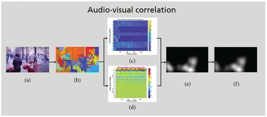
Figure 9.
Illustration of the audio-visual correlation analysis corresponding to a sample frame from the input video. (a) Frame F, (b) STRs extracted from frame F, (c) visual features (velocity and acceleration), (d) audio features (MFCC and MFCC-D), (e) correlation map between visual and audio features, and (f) audio attention map .
For further details on the KCCA framework and related mathematical analysis, the reader is referred to [5,33].
3.5. Creating the Final Audio-Visual Saliency Map
The final stage is the production of the final audio-visual saliency map. This involves the integration of face, spatial, temporal, and audio saliency maps.
S denotes the final audio-visual saliency map, whereas and represent the temporal and auditory saliency maps, respectively. refers to the static saliency map, which includes the spatial saliency map and face.
According to implicit memory theory, previous attentional targets guide attention paths in subsequent fixations. Therefore, in frames with largely unchanged context, individuals tend to focus on the same locations as in the previous frame. Typically, consecutive video frames exhibit minimal content variation, resulting in highly similar saliency maps across successive frames [40]. Consequently, regions identified as faces in the previous frame are expected to correspond to faces in the current frame. Building on this, we intersect the face saliency map of the previous frame with that of the current frame to correct potential face detection errors, obtaining as defined in Equation (20).
denotes the spatial attention map, represents the face saliency map in the current frame, and indicates the face saliency map in the previous frame, while ∧ signifies the logical operator.
To create the final audio-visual saliency map, we use the integration method described in [5] according to Equation (21).
where and are the temporal and spatial saliency weights, respectively, computed as per Equation (22). The saliency map is obtained by combining the spatial and temporal maps. An effective saliency map should display compact, clustered salient regions rather than scattered points. The coefficients and in Equation (21) control the contribution of the spatial and temporal maps, adjusting for their relative importance to ensure that maps with more salient information have a greater influence on the final integration. The term captures the combined effect of both maps, emphasizing regions with high saliency in both domains, as these are assumed to play a critical role in audio-visual attention.
The parameter acts as a tuning threshold, while denotes the average saliency intensity in map . A higher mean value indicates more concentrated and prominent salient regions, which are critical in the fusion process. When exceeds , the weight approaches 1, increasing the contribution of salient maps. Below the threshold, the weight decreases, reducing the influence of less salient maps. This formulation offers a flexible approach for integrating spatial and temporal information. The values of and are empirically determined from the baseline model in [5]. The weights and are adaptively computed, allowing dynamic adjustment based on the input data’s characteristics. The auditory and visual saliency maps are then integrated, considering the dependability of the audio saliency map.
A higher value of indicates that auditory saliency is concentrated in regions with strong motion, enhancing the reliability of the auditory map. In this case, plays a more significant role in the final integration. Conversely, a low suggests auditory saliency in regions with weak motion, resulting in less reliable auditory information, where visual saliency dominates the fusion process. The weight is computed as follows:
Here, is a matrix of the same size as the auditory saliency map , where pixels are set to 1 if and 0 otherwise, highlighting regions with significant auditory saliency. The term quantifies the correlation between auditory saliency and motion. A higher correlation increases , while a lower correlation decreases it. The parameter tunes the system’s sensitivity to this correlation, empirically set to 0.4 based on [5]. The model assumes that sound-generating objects are typically associated with motion. When auditory saliency aligns with significant motion, the auditory map is considered reliable; otherwise, it is regarded as noise. This adaptive fusion strategy adjusts the contribution of auditory saliency based on its correlation with motion, ensuring accurate audio-visual source detection while minimizing the impact of irrelevant noise.
Figure 10 presents the proposed saliency detection framework over time using three representative videos from the dataset. For each video, saliency maps are shown for three frames at different timestamps. Each row corresponds to a video frame, while columns display the original frame followed by spatial saliency, face saliency, temporal saliency, audio saliency, the final audio-visual saliency map, and the corresponding eye-tracking (gaze) data. This time-series visualization illustrates the temporal dynamics of audio-visual saliency, emphasizing the model’s response to static features, motion, facial presence, and auditory cues across varying scenes. Comparing the intermediate saliency maps with the final saliency and gaze data enables a more precise evaluation of the fusion process’s effectiveness and temporal behavior.
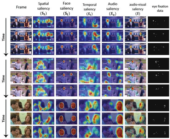
Figure 10.
Time-series visualization of audio-visual saliency detection results for three videos. Each row shows a selected frame over time, with columns displaying the original frame, saliency maps (spatial, face, temporal, and audio), the final audio-visual saliency map, and the corresponding eye fixation data. The figure highlights how different modalities contribute to saliency across time.
4. Results and Discussion
We evaluated the proposed method on the Audio-Visual Attention Dataset (AVAD), introduced in [39]. The dataset consists of 45 videos depicting diverse scenes that highlight various audio-visual processes. Each video lasts between 5 and 10 s and exhibits strong audio-visual correspondence. In most cases, the primary event in the scene produces a dominant sound. However, some videos feature motion without corresponding audio, such as pedestrians passing or conversational partners moving.
We compare our method to the baseline model [5] and visual saliency models. We also talk about ablation studies that look at the role of sound and other types of information in our model.
4.1. Comparison with Visual Attention Models
We compare our proposed model against three categories: audio-visual saliency models, static saliency models, and saliency prediction models for dynamic scenes.
- Static saliency models: The image saliency models designed for static scenes are as follows: IT, a saliency model derived from the neural structure of the primate early visual system [13]; GBVS, graph-based visual saliency [14]; SR, Fourier transform-based spectral residual saliency mode [16]; SUN, saliency using natural statistics [17]; FES, Visual Saliency Detection With Free Energy Theory [36]; HFT, a saliency model based the hypercomplex Fourier transform [42]; BMS, a Boolean map-based saliency model [43]; Judd, a supervised learning model of saliency incorporating bottom-up saliency cues and top-down semantic-dependent cues [44]; and SMVJ, a saliency model utilizing low-level saliency integrated with face detection [45].
- Dynamic saliency models: Video saliency models developed for dynamic scenes include the following: RWRV, saliency detection via random walk with restart [46]; SER, a model for static and space–time visual saliency detection using self-resemblance [47]; ICL, a dynamic visual attention model predicated on feature rarity [48]; and PQFT, Spatio-temporal Saliency Detection Employing the Phase Spectrum of the Quaternion Fourier Transform [41].
- Multimodal Model: the multimodal baseline model introduced in [5], an audio-visual attention model designed for predicting eye fixations.
For the evaluation of saliency models, we employed AUC-Borji, AUC-Judd [49], and NSS metrics [50]. The quantitative results are presented in Table 2, with values for static and dynamic saliency models sourced directly from [5]. The table reports the average performance across all video frames. The results indicate that the proposed model outperforms state-of-the-art image and video saliency models, as well as the baseline model, across all evaluation metrics. This highlights the importance of audio and facial features in capturing visual attention.
Table 2.
Comparison with state-of-the-art image and video saliency models. Bold values indicate the best performance for each metric. The upward arrow (↑) signifies that higher values correspond to better performance.
We conducted a paired t-test on data from 45 videos to evaluate the statistical significance of performance differences between the proposed and baseline models. The p-values, shown in Table 3, indicate that the proposed model consistently outperforms the baseline across all evaluation metrics (p < 0.05). The low p-values suggest that the improvements are unlikely to result from chance. These findings demonstrate that the proposed model effectively processes audio-visual features, yielding a more accurate representation of visual attention. Thus, the performance enhancement is both statistically and practically significant.
Table 3.
Paired t-test analysis of performance metrics for the proposed and baseline models.
4.2. Ablation Studies
To assess the impact of multimodal data, we conducted an ablation study on four variations of our approach. Let denote the total feature space, including , , , and , as shown in Table 4. In each round, we excluded one feature and reported the results in Table 5. For instance, indicates that we used , , and , excluding the audio saliency map from our model.
Table 4.
Our model variations.
Table 5.
Ablation studies. Bold values indicate the best performance for each metric.
The auditory saliency map () plays a crucial role in visual attention, as its removal leads to a significant decline in key performance metrics, particularly NSS and KL-Div. The concurrent decline in these metrics underscores the fundamental role of auditory cues in guiding visual attention, particularly in dynamic environments where sound localization enhances perceptual accuracy. Furthermore, our findings are consistent with previous research on multimodal saliency [7,10], reinforcing the necessity of incorporating auditory information for accurate eye movement prediction.
The spatial saliency map () is crucial, as the decline in evaluation metrics upon its removal underscores the importance of spatial information in predicting visual fixations. Despite other cues, removing reduces alignment with human eye movement patterns, emphasizing the role of static visual features.
The face saliency map () plays a context-dependent role in predicting visual fixations, enhancing performance in face-present scenarios. However, its removal does not significantly affect performance in face-absent settings. This suggests that face saliency is primarily beneficial in scenes containing human faces, supporting the importance of integrating targeted features. These results align with previous research on face-driven visual attention [30] and have implications for human–computer interaction, gaze prediction, and adaptive multimedia systems.
The removal of the temporal saliency map () has the least impact on performance, as our model encodes temporal information through alternative mechanisms. Specifically, the speed and range of light flow are captured by the auditory saliency map (), which simulates dynamic features. Consequently, removing does not significantly affect performance, indicating considerable overlap between motion- and sound-driven attention in saliency estimation. Future research could explore advanced motion saliency models that explicitly integrate multisensory cues to further optimize unified saliency prediction.
Table 5 confirms that our full model () achieves the best results across all metrics, indicating the effectiveness of integrating multisensory data. The complementary relationship between spatial, temporal, auditory, and facial features contributes to robust performance in diverse scenarios, consistent with previous studies on multimodal saliency.
4.3. Discussion
In this section, we present comparison charts to evaluate our method against the multimodal baseline model [5] using other evaluation criteria such as S, CC [51], and KL-D [50]. Figure 11 shows the comparison between the baseline and proposed models across six evaluation criteria.
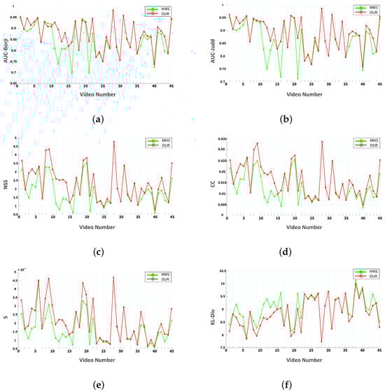
Figure 11.
Evaluation results of the proposed model and the MMS model with different evaluation criteria in the AVAD dataset. (a) AUC-Borji, (b) AUC-Judd, (c) NSS, (d) CC, (e) S, and (f) KL-Div.
For all metrics except KL-D, higher values indicate better alignment between the saliency map and ground-truth human fixations. A decrease in KL-D reflects a shift in the statistical distribution of saliency rather than a loss of spatial accuracy. Thus, it is important to interpret this metric alongside other evaluation measures [50].
Based on the content, dataset videos are categorized into three types.
Type (1): In these videos, multiple salient objects are present, but only one produces sound at any given moment. In this context, a human observer may focus not only on the sound-producing object but also on other regions, such as the face of a co-presenter in a news program (Figure 12, rows 3 and 4). By incorporating both low-level and high-level features alongside audio, the proposed model enhances the prominence of the sound-producing object and, through accurate localization, improves visual attention prediction accuracy.
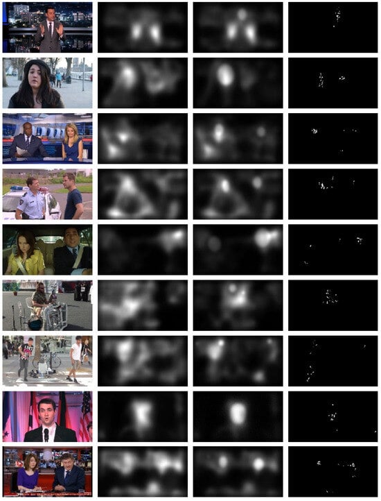
Figure 12.
Examples of related saliency maps. From the left: main frame, basic model output (MMS), proposed model output, eye fixation data.
Type (2): A moving object generates sound while background distractions, such as pedestrians, occur. In these scenarios, the sound-producing object is prominent both visually and auditorily (Figure 12, rows 3 and 4). Traditional saliency models may be compromised by background motion, whereas the proposed audio-visual model effectively mitigates these distractions and localizes the sound source.
Type (3): Similar to Type (2), this category includes a sound-producing object; however, there is no background movement. In these videos, the salient sound-producing object is unequivocally the focal point of visual attention. The proposed audio-visual model can enhance this focus. For example, in Figure 12, row 8, the news reporter is further emphasized through audio-visual analysis. For other videos in this category, the mechanism of the audio-visual attention model works similarly.
As discussed in Section 2.3, in some videos, the sound-producing element is less prominent than other regions. This reduced prominence may result from significant competing motion in other areas. In such cases, sound localization may yield inaccurate results, as shown in Figure 11 and Figure 12. However, the proposed model outperforms the baseline model in these situations.
Based on the data in Table 2 and Table 4, and Figure 11 and Figure 12, the proposed model outperforms the baseline and other saliency models on the AVAD dataset across most evaluation metrics. However, in real-world environments, auditory and visual cues are not always strongly correlated. Background noise or competing auditory signals can create ambiguity, challenging the model’s robustness. A key challenge is simulating human attention in cluttered scenes with dynamic auditory and visual stimuli. Future research should focus on improving simulations in such contexts and developing more accurate methods for identifying auditory sources, as enhanced localization could lead to more reliable auditory saliency maps. As discussed in the ablation study, our approach to temporal saliency estimation relies on frame differences. Future work could explore more advanced methods to improve accuracy in scenes with significant background motion noise and camera motion.
5. Conclusions
Scientific research has shown that visual information, auditory stimuli, and facial cues significantly influence human attention. Our sensory experience is multi-dimensional, and the interactions between these modalities guide attention. In this study, we present a computational–cognitive model of audio-visual attention. The model first detects spatial, face, and temporal saliency within the visual domain. Spatial saliency is extracted using the free energy principle, face saliency is identified via the MTCNN deep face detection algorithm, and temporal saliency is modeled based on inter-frame differences. Through visual-auditory correlation analysis, we identify moving, sound-producing objects and generate an audio attention map for each frame. Finally, leveraging the principle of expectation—that important elements in the current frame remain relevant in the next—we integrate these maps to form a final audio-visual saliency map. Our results highlight the importance of incorporating both sound information and low- and high-level visual information. Ablation studies demonstrate that sound significantly contributes to visual attention and is a critical component of multimedia content.
Additionally, faces are by far the most significant features influencing gaze behavior. The presence of faces significantly impacts visual exploration by drawing the most fixations toward them. Therefore, they should be considered an integral part of the saliency pathway. The performance of the generated audio-visual saliency maps is validated using video sequences and eye-tracking data.
Future research will focus on developing advanced models to predict auditory-visual attention in real-world applications, with an emphasis on reducing computational time and achieving real-time processing. However, the computational complexity of integrating multiple saliency cues may limit real-time applicability, requiring further optimization for use in interactive systems.
While this paper proposes an adaptive two-stage approach for integrating auditory and visual cues, optimal fusion may not always be achieved, especially in scenarios with weak or ambiguous correlations between the signals. Improving the fusion strategy to better balance spatial, temporal, and auditory features could enhance model performance in diverse and complex scenes. Moreover, exploring deep learning-based fusion strategies may further improve the model’s adaptability and generalizability. These challenges and future directions highlight the potential for advancing multimedia saliency prediction by combining traditional methods with modern deep learning techniques.
Author Contributions
H.Y. conducted the experiments and interpreted the results. A.B., R.E. and F.D. developed the research framework and roadmap and worked on the conceptualization. H.Y., A.B., R.E. and F.D. discussed and analyzed the results. All authors have read and agreed to the published version of the manuscript.
Funding
The project has received partial funding from Shahid Rajaee Teacher Training University under grant number 4891 and from the Cognitive Science and Technology Council under contract number 11410.
Data Availability Statement
The data supporting the findings of this investigation are accessible from the corresponding author, A. Bosaghzadeh, upon reasonable request.
Conflicts of Interest
The authors declare no conflicts of interest.
References
- Borji, A.; Itti, L. State-of-the-Art in Visual Attention Modeling. IEEE Trans. Pattern Anal. Mach. Intell. 2013, 35, 185–207. [Google Scholar] [CrossRef] [PubMed]
- Borji, A.; Ahmadabadi, M.N.; Araabi, B.N.; Hamidi, M. Online learning of task-driven object-based visual attention control. Image Vis. Comput. 2010, 28, 1130–1145. [Google Scholar] [CrossRef]
- Liu, Y.; Qiao, M.; Xu, M.; Li, B.; Hu, W.; Borji, A. Learning to predict salient faces: A novel visual-audio saliency model. In Proceedings of the Computer Vision–ECCV 2020: 16th European Conference, Glasgow, UK, 23–28 August 2020; Proceedings, Part XX 16. Springer: Berlin/Heidelberg, Germany, 2020; pp. 413–429. [Google Scholar] [CrossRef]
- Borji, A.; Cheng, M.M.; Jiang, H.; Li, J. Salient Object Detection: A Benchmark. IEEE Trans. Image Process. 2015, 24, 5706–5722. [Google Scholar] [CrossRef]
- Min, X.; Zhai, G.; Zhou, J.; Zhang, X.P.; Yang, X.; Guan, X. A Multimodal Saliency Model for Videos with High Audio-Visual Correspondence. IEEE Trans. Image Process. 2020, 29, 3805–3819. [Google Scholar] [CrossRef]
- Tsiami, A.; Koutras, P.; Maragos, P. STAViS: Spatio-Temporal AudioVisual Saliency Network. In Proceedings of the 2020 IEEE/CVF Conference on Computer Vision and Pattern Recognition (CVPR), Seattle, WA, USA, 13–19 June 2020; pp. 4765–4775. [Google Scholar] [CrossRef]
- Coutrot, A.; Guyader, N.; Ionescu, G.; Caplier, A. Influence of soundtrack on eye movements during video exploration. J. Eye Mov. Res. 2012, 5, 2. [Google Scholar] [CrossRef]
- Song, G.; Pellerin, D.; Granjon, L. Different types of sounds influence gaze differently in videos. J. Eye Mov. Res. 2013, 6, 1–13. [Google Scholar] [CrossRef]
- Min, X.; Zhai, G.; Gao, Z.; Hu, C.; Yang, X. Sound influences visual attention discriminately in videos. In Proceedings of the 2014 Sixth International Workshop on Quality of Multimedia Experience (QoMEX), Singapore, 18–20 September 2014; pp. 153–158. [Google Scholar] [CrossRef]
- Tavakoli, H.R.; Borji, A.; Rahtu, E.; Kannala, J. DAVE: A Deep Audio-Visual Embedding for Dynamic Saliency Prediction. arXiv 2019, arXiv:1905.10693. [Google Scholar] [CrossRef]
- Treisman, A.M.; Gelade, G. A feature-integration theory of attention. Cogn. Psychol. 1980, 12, 97–136. [Google Scholar] [CrossRef]
- Koch, C.; Ullman, S. Chapter 1—Shifts in selective visual attention: Towards the underlying neural circuitry. In Matters of Intelligence: Conceptual Structures in Cognitive Neuroscience; Springer: Dordrecht, The Netherlands, 1987; pp. 115–141. [Google Scholar] [CrossRef]
- Itti, L.; Koch, C.; Niebur, E. A model of saliency-based visual attention for rapid scene analysis. IEEE Trans. Pattern Anal. Mach. Intell. 1998, 20, 1254–1259. [Google Scholar] [CrossRef]
- Harel, J.; Koch, C.; Perona, P. Graph-Based Visual Saliency. In Proceedings of the 19th International Conference on Neural Information Processing Systems (NIPS’06), Cambridge, MA, USA, 4 December 2006; pp. 545–552. [Google Scholar]
- Riche, N.; Mancas, M. Bottom-Up Saliency Models for Still Images: A Practical Review. In From Human Attention to Computational Attention: A Multidisciplinary Approach; Springer: New York, NY, USA, 2016; pp. 141–175. [Google Scholar]
- Hou, X.; Zhang, L. Saliency Detection: A Spectral Residual Approach. In Proceedings of the 2007 IEEE Conference on Computer Vision and Pattern Recognition, Minneapolis, MN, USA, 17–22 June 2007; pp. 1–8. [Google Scholar] [CrossRef]
- Zhang, L.; Tong, M.H.; Marks, T.K.; Shan, H.; Cottrell, G.W. SUN: A Bayesian framework for saliency using natural statistics. J. Vis. 2008, 8, 32. [Google Scholar] [CrossRef]
- Farkish, A.; Bosaghzadeh, A.; Amiri, S.H.; Ebrahimpour, R. Evaluating the Effects of Educational Multimedia Design Principles on Cognitive Load Using EEG Signal Analysis. Educ. Inf. Technol. 2023, 28, 2827–2843. [Google Scholar] [CrossRef]
- Wang, Y.; Liu, Z.; Xia, Y.; Zhu, C.; Zhao, D. Spatiotemporal module for video saliency prediction based on self-attention. Image Vis. Comput. 2021, 112, 104216. [Google Scholar] [CrossRef]
- Fang, Y.; Wang, Z.; Lin, W.; Fang, Z. Video Saliency Incorporating Spatiotemporal Cues and Uncertainty Weighting. IEEE Trans. Image Process. 2014, 23, 3910–3921. [Google Scholar] [CrossRef] [PubMed]
- Wang, W.; Shen, J.; Shao, L. Consistent Video Saliency Using Local Gradient Flow Optimization and Global Refinement. IEEE Trans. Image Process. 2015, 24, 4185–4196. [Google Scholar] [CrossRef]
- Liu, Z.; Li, J.; Ye, L.; Sun, G.; Shen, L. Saliency Detection for Unconstrained Videos Using Superpixel-Level Graph and Spatiotemporal Propagation. IEEE Trans. Circuits Syst. Video Technol. 2017, 27, 2527–2542. [Google Scholar] [CrossRef]
- Rogalska, A.; Napieralski, P. The visual attention saliency map for movie retrospection. Open Phys. 2018, 16, 188–192. [Google Scholar] [CrossRef]
- Bosaghzadeh, A.; Shabani, M.; Ebrahimpour, R. A Computational-Cognitive model of Visual Attention in Dynamic Environments. J. Electr. Comput. Eng. Innov. 2021, 10, 163–174. [Google Scholar] [CrossRef]
- Wang, W.; Shen, J.; Porikli, F. Saliency-aware geodesic video object segmentation. In Proceedings of the 2015 IEEE Conference on Computer Vision and Pattern Recognition (CVPR), Boston, MA, USA, 7–12 June 2015; pp. 3395–3402. [Google Scholar] [CrossRef]
- Wang, W.; Shen, J.; Yang, R.; Porikli, F. Saliency-Aware Video Object Segmentation. IEEE Trans. Pattern Anal. Mach. Intell. 2018, 40, 20–33. [Google Scholar] [CrossRef]
- Koutras, P.; Katsamanis, A.; Maragos, P. Predicting Eyes’ Fixations in Movie Videos: Visual Saliency Experiments on a New Eye-Tracking Database. In Engineering Psychology and Cognitive Ergonomics, Proceedings of the 11th International Conference, EPCE 2014, Held as Part of HCI International 2014, Heraklion, Crete, Greece, 22–27 June 2014; Harris, D., Ed.; Springer International Publishing: Cham, Switzerland, 2014; pp. 183–194. [Google Scholar]
- Wang, G.; Chen, C.; Fan, D.; Hao, A.; Qin, H. From Semantic Categories to Fixations: A Novel Weakly-supervised Visual-auditory Saliency Detection Approach. In Proceedings of the 2021 IEEE/CVF Conference on Computer Vision and Pattern Recognition (CVPR), Los Alamitos, CA, USA, 19–25 June 2021; pp. 15114–15123. [Google Scholar] [CrossRef]
- Chen, C.; Song, M.; Song, W.; Guo, L.; Jian, M. A Comprehensive Survey on Video Saliency Detection with Auditory Information: The Audio-visual Consistency Perceptual is the Key! IEEE Trans. Circuits Syst. Video Technol. 2022, 33, 457–477. [Google Scholar] [CrossRef]
- Ashwini, P.; Ananya, K.; Nayaka, B.S. A Review on Different Feature Recognition Techniques for Speech Process in Automatic Speech Recognition. Int. J. Sci. Technol. Res. 2019, 8, 1953–1957. [Google Scholar]
- Kayser, C.; Petkov, C.I.; Lippert, M.; Logothetis, N.K. Mechanisms for Allocating Auditory Attention: An Auditory Saliency Map. Curr. Biol. 2005, 15, 1943–1947. [Google Scholar] [CrossRef] [PubMed]
- Izadinia, H.; Saleemi, I.; Shah, M. Multimodal Analysis for Identification and Segmentation of Moving-Sounding Objects. IEEE Trans. Multimed. 2013, 15, 378–390. [Google Scholar] [CrossRef]
- Hardoon, D.R.; Szedmak, S.; Shawe-Taylor, J. Canonical correlation analysis: An overview with application to learning methods. Neural Comput. 2004, 16, 2639–2664. [Google Scholar] [CrossRef] [PubMed]
- Zhai, G.; Wu, X.; Yang, X.; Lin, W.; Zhang, W. A Psychovisual Quality Metric in Free-Energy Principle. IEEE Trans. Image Process. 2012, 21, 41–52. [Google Scholar] [CrossRef] [PubMed]
- Friston, K. The free-energy principle: A unified brain theory? Nat. Reviews Neurosci. 2010, 11, 127–138. [Google Scholar] [CrossRef]
- Gu, K.; Zhai, G.; Lin, W.; Yang, X.; Zhang, W. Visual Saliency Detection With Free Energy Theory. IEEE Signal Process. Lett. 2015, 22, 1552–1555. [Google Scholar] [CrossRef]
- Coutrot, A.; Guyader, N. How saliency, faces, and sound influence gaze in dynamic social scenes. J. Vis. 2014, 14, 5. [Google Scholar] [CrossRef]
- Zhang, K.; Zhang, Z.; Li, Z.; Qiao, Y. Joint Face Detection and Alignment Using Multitask Cascaded Convolutional Networks. IEEE Signal Process. Lett. 2016, 23, 1499–1503. [Google Scholar] [CrossRef]
- Min, X.; Zhai, G.; Gu, K.; Yang, X. Fixation Prediction through Multimodal Analysis. ACM Trans. Multimed. Comput. Commun. Appl. 2016, 13, 1–23. [Google Scholar] [CrossRef]
- Fang, Y.; Lin, W.; Chen, Z.; Tsai, C.M.; Lin, C.W. A Video Saliency Detection Model in Compressed Domain. IEEE Trans. Circuits Syst. Video Technol. 2014, 24, 27–38. [Google Scholar] [CrossRef]
- Guo, C.; Ma, Q.; Zhang, L. Spatio-temporal Saliency detection using phase spectrum of quaternion fourier transform. In Proceedings of the 2008 IEEE Conference on Computer Vision and Pattern Recognition, Anchorage, AK, USA, 23–28 June 2008; pp. 1–8. [Google Scholar] [CrossRef]
- Li, J.; Levine, M.D.; An, X.; Xu, X.; He, H. Visual Saliency Based on Scale-Space Analysis in the Frequency Domain. IEEE Trans. Pattern Anal. Mach. Intell. 2013, 35, 996–1010. [Google Scholar] [CrossRef] [PubMed]
- Zhang, J.; Sclaroff, S. Saliency Detection: A Boolean Map Approach. In Proceedings of the IEEE International Conference on Computer Vision (ICCV), Sydney, Australia, 1–8 December 2013. [Google Scholar] [CrossRef]
- Judd, T.; Ehinger, K.; Durand, F.; Torralba, A. Learning to predict where humans look. In Proceedings of the 2009 IEEE 12th International Conference on Computer Vision, Kyoto, Japan, 29 September–2 October 2009; pp. 2106–2113. [Google Scholar] [CrossRef]
- Cerf, M.; Harel, J.; Einhaeuser, W.; Koch, C. Predicting human gaze using low-level saliency combined with face detection. In Advances in Neural Information Processing Systems; Platt, J., Koller, D., Singer, Y., Roweis, S., Eds.; Curran Associates, Inc.: New York, NY, USA, 2007; Volume 20. [Google Scholar]
- Kim, H.; Kim, Y.; Sim, J.Y.; Kim, C.S. Spatiotemporal Saliency Detection for Video Sequences Based on Random Walk With Restart. IEEE Trans. Image Process. 2015, 24, 2552–2564. [Google Scholar] [CrossRef] [PubMed]
- Seo, H.J.; Milanfar, P. Static and space-time visual saliency detection by self-resemblance. J. Vis. 2009, 9, 15. [Google Scholar] [CrossRef] [PubMed]
- Hou, X.; Zhang, L. Dynamic visual attention: Searching for coding length increments. In Advances in Neural Information Processing Systems; Koller, D., Schuurmans, D., Bengio, Y., Bottou, L., Eds.; Curran Associates, Inc.: New York, NY, USA, 2008; Volume 21. [Google Scholar]
- Riche, N.; Duvinage, M.; Mancas, M.; Gosselin, B.; Dutoit, T. Saliency and Human Fixations: State-of-the-Art and Study of Comparison Metrics. In Proceedings of the IEEE International Conference on Computer Vision (ICCV), Sydney, Australia, 1–8 December 2013. [Google Scholar] [CrossRef]
- Emami, M.; Hoberock, L.L. Selection of a best metric and evaluation of bottom-up visual saliency models. Image Vis. Comput. 2013, 31, 796–808. [Google Scholar] [CrossRef]
- Bylinskii, Z.; Judd, T.; Oliva, A.; Torralba, A.; Durand, F. What Do Different Evaluation Metrics Tell Us About Saliency Models? IEEE Trans. Pattern Anal. Mach. Intell. 2019, 41, 740–757. [Google Scholar] [CrossRef]
Disclaimer/Publisher’s Note: The statements, opinions and data contained in all publications are solely those of the individual author(s) and contributor(s) and not of MDPI and/or the editor(s). MDPI and/or the editor(s) disclaim responsibility for any injury to people or property resulting from any ideas, methods, instructions or products referred to in the content. |
© 2025 by the authors. Licensee MDPI, Basel, Switzerland. This article is an open access article distributed under the terms and conditions of the Creative Commons Attribution (CC BY) license (https://creativecommons.org/licenses/by/4.0/).