A Formal Model of Trajectories for the Aggregation of Semantic Attributes

Abstract

A trajectory is a set of time-stamped locations of a moving object usually recorded by GPS sensors. Today, an abundance of these data is available. These large quantities of data need to be analyzed to determine patterns and associations of interest to business analysts. In this paper, a formal model of trajectories is proposed, which focuses on the aggregation of semantic attributes. These attributes can be associated by the analyst to different structural elements of a trajectory (either to the points, to the edges, or to the entire trajectory). The model allows the analyst to specify not only these semantic attributes, but also to specify for each semantic attribute the set of aggregation operators (SUM, AVG, MAX, MIN, etc.) that the analyst considers appropriate to be applied to the attribute in question. The concept of PAV (package of aggregate values) is also introduced and formalized. PAVs can help identify patterns in traffic, tourism, migrations, among other fields. Experiments with real data about trajectories of people revealed interesting findings about the way people move and showed the expediency and usefulness of the proposal. The contributions in this work provide a foundation for future research in developing trajectory applications including analysis and visualization of trajectory aggregated data based on formal grounds.

1. Introduction

According to [1], a trajectory is the record of the evolution of the position (point) of an object that is moving in space during a given time interval to achieve a specific goal. In real life scenarios, trajectories of moving objects are usually made up of thousands of points (also called observations or coordinates). Let us consider, for example, a trucking company. Each truck during its journey generates, e.g., every minute, geo-positioned data. Considering 10 h of operation as the daily trajectory of a truck, in one day, a truck produces 36,000 points. Assuming a fleet of n trucks, to analyze one year of operation, there are approximately 365 * n trajectories and each trajectory has about 36,000 points. Analyzing these large sets of data (big data) to determine patterns and associations of interest to business analysts can help identify traffic problems at certain times (rush hours), plan truck dispatch schedules to save fuel (get to the destination faster, avoid traffic jams), detect potential relationships between environmental conditions (temperature, humidity, pollution, wind speed, among others), and the performance of drivers and trucks, among other aspects.

Given a set of trajectories, the analysis is usually focused on a specific region (cell) of space and a specific time interval, i.e., a spatio-temporal cell. The goal is to obtain statistics and aggregate values corresponding to the trajectories (or subtrajectories) that occurred in that spatio-temporal cell. This approach allows the comparison and search for patterns between different spatio-temporal cells. An example is comparing the number of different trajectories that visited two adjacent cells in space in two consecutive time intervals to analyze, e.g., the propagation (flow) of trajectories from one cell to another, or to detect the most visited cells in a given time interval.

In addition, as expressed in [2], a line of research is to obtain the aggregate trajectory (the “representative” trajectory) from the set of trajectories, which occurred, e.g., in a given spatio-temporal cell. This problem involves answering questions such as (i) what does it mean to sum or average a set of trajectories? and (ii) what is the minimum or maximum trajectory of a set of trajectories?

It is also possible to obtain aggregate values of semantic attributes associated with a trajectory. For example, if the temperature at each point (or at most of the points) of a trajectory is available, then given a set of trajectories that occurred in a spatio-temporal cell, it is possible to obtain the maximum and minimum temperature recorded and the average of the temperatures, among other possible measures. Similarly, if trajectories of tourists are considered and the means of locomotion they used between consecutive points of their trajectories are available, it is possible to obtain which was the most used means of locomotion and what was the average distance and time travelled between two consecutive points. The above suggests that a trajectory may have associated semantic attributes at each of its points and at its edges (an edge is defined by two consecutive points of a trajectory).

On the other hand, there may also be semantic attributes associated to the entire trajectory, e.g., the number plate of a truck remains the same throughout a trajectory; in fact, it is the same for all its trajectories during its lifetime. Thus, given a set of trajectories of different trucks that occurred in a spatio-temporal cell, it is possible to obtain, for example, the number (count) of different license plates (trucks).

In this paper, a formal model of trajectories is proposed focused on the aggregation of semantic attributes which can be associated by the analyst to different structural elements of a trajectory (either to the points, to the edges, or to the entire trajectory). The model allows the analyst to specify not only these semantic attributes, allowing them to be placed in the appropriate structural element, but also to specify for each semantic attribute the set of aggregation operators (SUM, AVG, MAX, MIN, etc.) that the analyst considers appropriate to be applied (logically correct, e.g., it may not make sense to add temperatures, but it makes sense to average them or to find their maximum or minimum) to the attribute in question. We also introduce and formalize the concept of PAV (package of aggregate values) for a spatio-temporal cell.

To the best of our knowledge, this proposal is the first to present a formalization focused on the aggregation of semantic attributes of trajectories. The most similar works, as can be seen in Section 2, have focused on methods for calculating the number of distinct trajectories that have visited a given spatio-temporal cell (composed of smaller cells in which this measure has been previously calculated). Other related works have focused on generating clusters of trajectories or merging a set of trajectories, seen again in Section 2, or on facilitating their visualization; see, e.g., [3,4], among others.

This article is organized as follows. In Section 2, related work is discussed and the formal model of trajectories for the aggregation of semantic attributes is presented in Section 3. Section 4 describes the experiments which were carried out. Conclusions and future research directions are outlined in the last section.

2. Related Works

In trajectory aggregation, a hot topic is to find the number of moving objects in a given region (“the query region”), e.g., in a square cell at a given time interval. This aggregation measure, called “presence” by some authors [5], is useful, e.g., to predict the movement of moving objects, which has applications, e.g., in vehicular traffic and tourism.

In [6], the problem of the presence calculation is addressed (although the authors do not use this term). The space is partitioned into cells. Initially, a process is run that calculates the presence in each cell. Four other measures are also calculated for each cell: the number of subsequent trajectories visiting adjacent cells (left, right, up, and down). With these five measures, a formula is proposed to calculate, approximately, the presence in a region R (which is composed of adjacent cells). Informally, the formula (i) obtains the sum of the presence of the cells that compose R, (ii) obtains the sum of all adjacency measures (left, right, up, and down) of the cells that compose R, and (iii) subtracts the value obtained in step (ii) from the value obtained in step (i), and this is the presence (although it may generate inaccurate results) of R. The authors then incorporate the temporal dimension, so that the presence of a cell in a time interval TI can be calculated. The procedure is essentially the same, except that the measures of each cell are calculated considering TI. A sixth measure, called stay, is also added, which indicates the number of trajectories that visited a cell during TI and did not leave the cell during that time interval.

Two methods are proposed in [7] and in its extended version [5] to calculate the presence measure, which computes the number of distinct trajectories passing through a given spatio-temporal region. The space is divided into spatio-temporal cells. Initially, a process is executed that calculates the presence in each cell. After this process, the goal is to calculate the presence in a region R, formed from the union of adjacent cells, considering the presence of the cells that compose R. The proposed methods to calculate the presence in R are as follows:

• Distributive: In this method, it is assumed that the only measure stored in each cell is its presence. To calculate the presence of R, the presences of the cells that compose R are added. Note that, in this method, if the same trajectory passes, e.g., through two cells that compose R, then this trajectory is counted twice; therefore, this method may produce inaccurate results.
• Algebraic: In this method, it is assumed that in addition to the presence, three additional measures (calculated by a previous process) are stored in each cell: (i) the number of distinct trajectories crossing the spatial border (i.e., the common border, perpendicular to the X-axis, of two adjacent cells) between two adjacent cells, (ii) same as (i) but for the border, perpendicular to the Y-axis, and (iii) same as (i) but for the temporal border between two adjacent cells, e.g., if a cell is defined in the intervals (8 am, 10 am] and (10 am, 12 m], then the temporal border occurs at 10 am. Based on these four measures, the presence of R is calculated. For example, to calculate the presence of two adjacent cells that have in common a border perpendicular to the X-axis, their presences are added and the number of distinct trajectories crossing such border is subtracted. This method, although more accurate than the distributive method, can also generate inaccurate results.

In [8] and in its extended version [9], an extension to the GROUP BY clause of SQL is proposed for the aggregation of trajectories together with an aggregation operator called AGGREGATE. A trajectory is a sequence of coordinates (x, y, t) associated to a moving object identified by a tag. The authors define three aggregation methods, GROUP BY OVERLAP, GROUP BY INTERSECTION, and GROUP BY INTERSECTION AND OVERLAPS. In summary, the GROUP BY OVERLAP method combines sequential trajectories and the GROUP BY INTERSECTION method combines parallel trajectories.

From the experiments conducted with school bus trajectories and with different thresholds, the authors highlight that the thresholds allow to control the size of the aggregation groups, i.e., to generate aggregation groups with fewer or more trajectories.

The presence problem has also been addressed in [10,11] with several variants, some of them very specialized [12]. For example, in [12], a method is proposed to calculate the number of moving objects, with a probability greater than a given probability, in some road sections (contained in a given region) and in a given time interval. The method proposed there has the following characteristics:

−

It supports uncertainty, i.e., given two consecutive points (x, y, t) of a trajectory, if between these two points, there are several road sections, it is unknown which of these road sections the moving object followed. That is, the method considers sparse trajectory samples.

−

It considers the problem of repetition counting, i.e., when a moving object visits the same region multiple times, to avoid counting it several times. For this reason, the authors use indexes and specialized data structures (histograms, hash tables, B+ trees, among others) to achieve a good level of accuracy and obtain it efficiently. The experimental results showed that the method ensures accuracy by adjusting some parameters.

In [13], the authors present an algorithm for center-based trajectory clustering. In center-based clustering, all objects in a cluster are close to one central object (called the center of the cluster). Therefore, for trajectory clustering, it is necessary to define a measure for computing the closeness (similarity) of two trajectories. For this purpose, the authors use the Fréchet distance [14], a measure of similarity between two curves. They apply their algorithm to 168 trajectories of pigeons and show visually that the center trajectories are “truthful” representations of their corresponding cluster.

In a similar work, Brankovic et al. [15] also consider the problem of center-based clustering of trajectories but using a different distance for computing the trajectories similarity. The authors propose a modified version of the dynamic time warping (DTW) distance measure. They call their measure continuous DTW (CDTW). In DTW, only vertices of the trajectory are considered (the edges between vertices are ignored). As such, DTW is sensitive to the sampling rate. On the other hand, the Fréchet distance may be sensitive to outliers. According to the results of their experiments, with trajectories of handwritten characters, pigeons, and storks, when clustering trajectories under the CDTW measure, the CDTW outperforms and overcomes the shortcomings of DTW and Fréchet distance.

In [16], an algorithm for privately aggregating a set of trajectories is proposed. Their goal is to generate a curve (in the two-dimensional space) that corresponds to an aggregate trajectory while ensuring differential privacy (DP). DP is notion of privacy which seeks to ensure that the output of an algorithm does not change noticeably if the data of a single element (e.g., a trajectory of a specific bus) are added or removed from the dataset. The authors demonstrate the effectiveness of their proposal with real-world datasets (trajectories of pigeons and New York buses), showing that it gives accurate results according to the adjustment of different parameters that they define for their algorithm.

Trajectory prediction is treated in [17] in the context of autonomous driving to forecast movements of vehicles. The authors propose a framework for aggregation of multiple trajectory predictors (TPs). A TP outputs a distribution representing predicted trajectories. Each TP is used to derive a combined predictive model known as a Mixture of Experts (MoE). MoE is evaluated using metrics such as the Minimum Average Displacement Error (minADE), which focuses on the average displacement between predicted and true trajectories, and the Minimum Final Displacement Error (minFDE), which focuses on the displacement between the predicted and the true endpoints of trajectories. Two datasets and three trajectory prediction models were considered. The results show that the MoE outperformed any individual TP. However, the aggregation of multiple TPs comes at the cost of running several models. Only three TPs were aggregated; future work should investigate the aggregation of more TPs.

A method for transforming raw trajectory data into a traffic flow map is proposed in [18]. The central idea is a process of comparing and aligning trajectory segments to identify common flow patterns. This process includes (i) breaking down trajectories into smaller segments, (ii) calculating similarity measures between these segments, and (iii) iteratively grouping and aligning similar segments to form representative flow lines. Thus, each flow line can be considered a representative subtrajectory of a set of segments from different trajectories. The method is applied to both synthetic and empirical trajectory datasets. The resulting traffic flow maps show high levels of accuracy, provide a clear and intuitive visualization of traffic patterns, and allow for capturing fine-grained variations in traffic flow. The authors state that their method can be computationally expensive (especially for large datasets) and that its performance may depend on the choice of parameters, such as the segment length and similarity threshold.

In

Table 1. Summary of works.

Reference (Year)	Contribution	Limitation
[6] (2002)	An efficient method for calculating the presence in a spatio-temporal cell.	- The method may generate inaccurate results. - It only focuses on the presence calculation.
[5,7] (2007)	Two efficient methods for calculating the presence in a spatio-temporal cell.	- The methods may generate inaccurate results. - They only focus on the presence calculation.
[8,9] 2008	An extension to the GROUP BY clause of SQL for aggregating trajectories.	- The method aggregates trajectories based only on their spatio-temporal coordinates. - Aggregation based on semantic attributes is not considered.
[11,12] 2014–2019	Probabilistic methods for calculating the presence in road sections in a time interval.	- The methods are specialized for road sections. - The methods focus only on the presence calculation.
[13] 2019	Trajectory clustering based on the Fréchet distance.	- The method creates clusters of trajectories based only on their spatio-temporal coordinates. - Clustering or aggregation based on semantic attributes is not considered.
[15] 2020	Trajectory clustering based on the continuous dynamic time warping distance.	- The method creates clusters of trajectories based only on their spatio-temporal coordinates. - Clustering or aggregation based on semantic attributes is not considered.
[16] 2022	A method for aggregating trajectories in a curve.	- The method generates a curve for a set of trajectories based only on their spatio-temporal coordinates. - Semantic attributes are not considered in this process.
[17] 2024	A model for aggregating multiple trajectory predictors (TPs).	- The method generates a predicted trajectory based on multiple TPs and on spatio-temporal coordinates. - Semantic attributes are not considered in this process.
[18] 2025	A method for aggregating a set of segments from different trajectories into a traffic flow map.	- The method generates flow lines (based only on the spatio-temporal coordinates) from a set of segments of trajectories. - Semantic attributes are not considered in this process.

, a summary of these works is presented.

3. A Formal Model of Trajectories for the Aggregation of Semantic Attributes

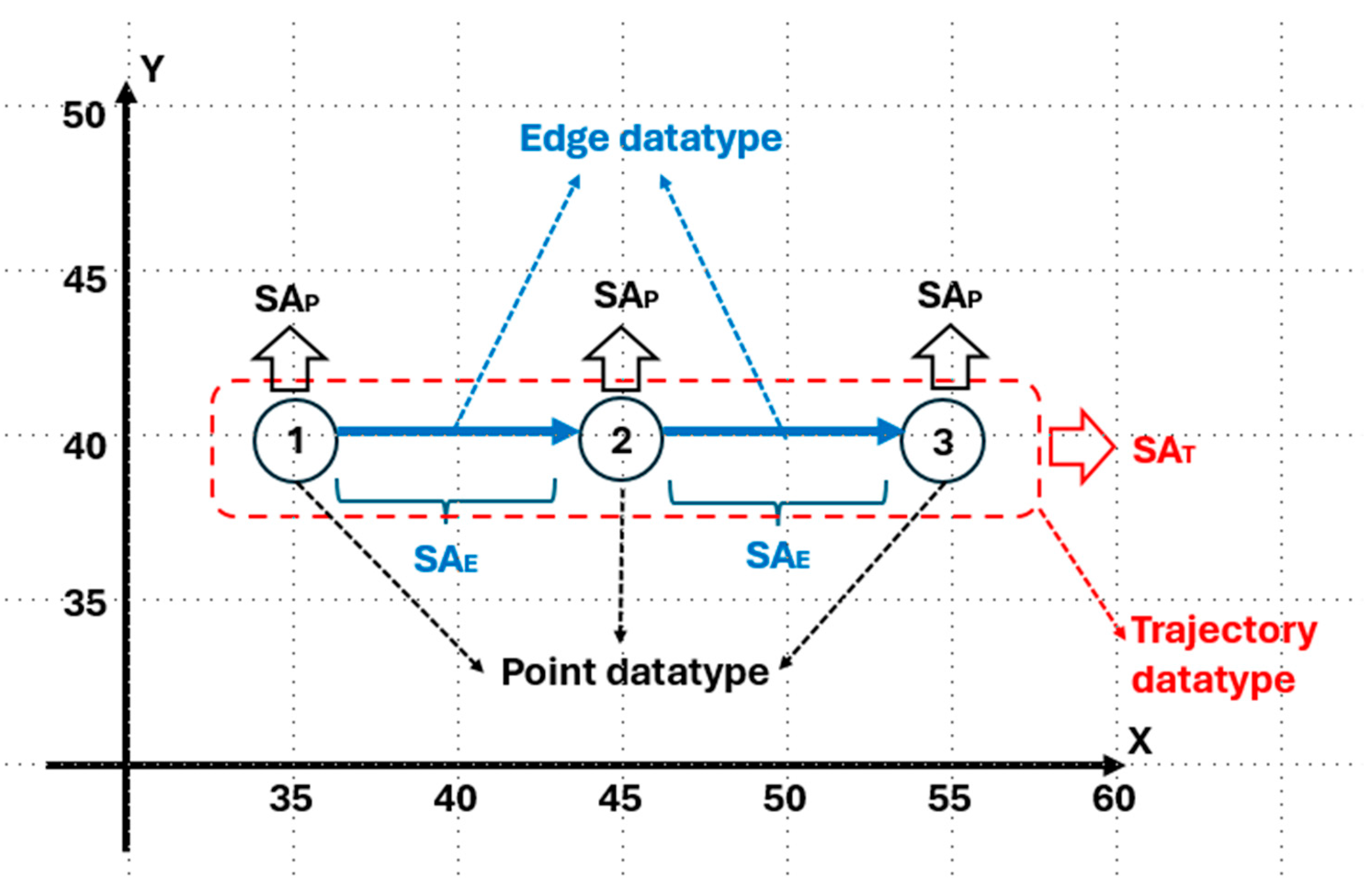
3.1. Basic Datatypes and Attributes

Let DT be the set of all datatypes of the trajectory database, e.g., DT = {Boolean, Geometry, Latitude, Longitude, R, R⁺, R⁻, String, Time Interval, Timestamp, Z, Z⁺, Z⁻, …}, where R stands for real datatype and Z stands for integer datatype.

Let ATTR be the set of all attributes of the trajectory database, e.g., ATTR = {busy, distance, gasolineLevel, numberofPassengers, passengersActivity, vehicleType, …}.

Let DTF be a function that returns the datatype of an attribute. Then, the prototype of DTF is ATTR → DT.

• Example:

DTF(busy) = Boolean, DTF(distance) = Z⁺, DTF(gasolineLevel) = Z⁺, DTF(numberofPassengers) = Z⁺, DTF(passengersActivity) = String, and DTF(vehicleType) = String.

3.2. Point Datatype

A point datatype Pdt is a tuple Pdt = (PointId, x, y, t, SA_P) where

(i)

PointId is the point identifier, DTF(PointId) = Z⁺.

(ii)

x represents the point latitude, DTF(x) = Latitude. For simplicity, in our examples, x is just a positive integer (in a Cartesian coordinate system), i.e., DTF(x) = Z⁺.

(iii)

y represents the point longitude, DTF(y) = Longitude. For simplicity, in our examples, y is just a positive integer (in a Cartesian coordinate system), i.e., DTF(y) = Z⁺.

(iv)

t is the point time, DTF(t) = Timestamp.

That is, x, y, and t represent the spatio-temporal coordinates of a point. These three attributes are the basic (raw) attributes of a point. Now, we consider additional (semantic) attributes that a point may have:

(v)

SA_P is a set of semantic attributes, SA_P = {sap₁, sap₂, …, sap_n}. Each semantic attribute has its corresponding datatype DTF(sap_i), for i = 1, …, n. For example, if SA_P = {busy, gasolineLevel, numberofPassengers}, then DTF(busy) = Boolean, DTF(gasolineLevel) = Z⁺, and DTF(numberofPassengers) = Z⁺.

3.3. Aggregation Functions for the Semantic Attributes of a Point Datatype

Let AggFsap_i be a set of aggregate functions AggFsap_i = {aggf₁, aggf₂, …, aggf_m} that are valid to be applied (according to the analyst) to an attribute sap_i ∈ SA_P, for i = 1, …, n; where n = Card(SA_P). Examples of aggregate functions are SUM, AVG, MAX, MIN, MODE (the most frequent value), STDDEV (standard deviation), among others.

• Example:

If SA_P = {busy, gasolineLevel, numberofPassengers}, then suppose AggFbusy = ø, AggFgasolineLevel = {AVG}, and AggFnumberofPassengers = {AVG, SUM}.

Thus, in this example, the analyst considers that it does not make sense to apply any aggregate function to a multiset (a collection) of busy values (of Boolean datatype). On the other hand, the analyst considers that it is valid to average (AVG) a multiset of gasoline level values (of Z⁺ datatype) and to add (SUM) and to average (AVG) a multiset of number of passengers’ values (of Z⁺ datatype).

The prototype of an aggregate function aggf_j ∈ AggFsap_i, for j = 1, …, m; where m = Card(AggFsap_i), sap_i ∈ SA_P, for i = 1, …, n; where n = Card(SA_P) is as follows:

M(DTF(sap_i)) → DTF(aggf_j)

where M(DTF(sap_i)) = {mt: mt is a multiset with elements from DTF(sap_i)}, i.e., M(DTF(sap_i)) is the set of all multisets that can be formed with elements of the datatype DTF(sap_i). DTF(aggf_j) is the resulting datatype of applying the aggf_j function to a multiset of values (a multiset ∈ M(DTF(sap_i))), each value of DTF(sap_i) datatype. That is, the aggf_j function takes a multiset of values (each value of DTF(sap_i) datatype) as input and generates a value of DTF(aggf_j) datatype as output.

• Example:

Consider AggFnumberofPassengers = {AVG, SUM}. Let us assume that DTF(numberofPassengers) = Z⁺. Now, consider the aggregate function SUM ∈ AggFnumberofPassengers, then DTF(SUM) = Z⁺, i.e., the sum of a multiset of positive integers (numberofPassengers) generates a positive integer as output. On the other hand, for the aggregate function AVG ∈ AggFnumberofPassengers, then, DTF(AVG) = R⁺, i.e., the average of a multiset of positive integers (numberofPassengers) generates a real (number) as output.

3.4. Edge Datatype

An edge datatype Edt is a tuple Edt = (PointId₁, PointId₂, SA_E) where

(i)

PointId₁ is the identifier of a point, DTF(PointId₁) = Z⁺.

(ii)

PointId₂ is the identifier of a point, DTF(PointId₂) = Z⁺.

(iii)

SA_E is a set of semantic attributes, SA_E = {sae₁, sae₂, …, sae_n}. Each semantic attribute has its corresponding datatype DTF(sae_i), for i = 1, …, n. For example, if SA_E = {distance, passengersActivity}, then DTF(distance) = R⁺ and DTF(passengersActivity) = String.

3.5. Aggregation Functions for the Semantic Attributes of an Edge Datatype

In a similar way to the aggregate functions for the semantic attributes of a point datatype, we define a set AggFsae_i of aggregate functions AggFsae_i = {aggf₁, aggf₂, …, aggf_m} that are valid to be applied (according to the analyst) to an attribute sae_i ∈ SA_E, for i = 1, …, n.

• Example:

If SA_E = {distance, passengersActivity}, then suppose AggFdistance = {SUM} and AggFpassengersActivity = {MODE}.

Thus, in this example, the analyst considers that it is valid to add (SUM) a multiset of distance values (of Z⁺ datatype) and that it is valid to find the most frequent value (MODE) of a multiset of passengers’ activity values (of String datatype).

The prototype of an aggregate function applied to a semantic attribute of an edge datatype is analogous to the prototype presented for the semantic attribute of a point, i.e., the prototype of an aggregate function aggf_j ∈ AggFsae_i, for j = 1, …, m; where m = Card(AggFsae_i), sae_i ∈ SA_E, for i = 1, …, n; where n = Card(SA_E) is

M(DTF(sae_i)) → DTF(aggf_j);

where M(DTF(sae_i)) = {mt: mt is a multiset with elements from DTF(sae_i), i.e., M(DTF(sae_i)) is the set of all multisets that can be formed with elements of the datatype DTF(sae_i).

• Example:

Consider AggFdistance = {SUM}. Let us assume that DTF(distance) = Z⁺. Now, consider the aggregate function SUM ∈ AggFdistance, then DTF(SUM) = Z⁺, i.e., the sum of a multiset of positive integers (distance) generates a positive integer as output. For AggFpassengersActivity = {MODE}, let us assume that DTF(passengersActivity) = String and for the aggregate function MODE ∈ AggFpassengersActivity, then DTF(MODE) = String, i.e., the most frequent value of a multiset of strings (passengersActivity) generates a String as output.

3.6. Trajectory Datatype

A trajectory datatype Tdt is a tuple Tdt = (TrajId, PDT, EDT, SA_T) where

(i)

TrajId is the identifier of a trajectory, DTF(TrajId) = Z⁺.

(ii)

PDT is a set of point datatypes, PDT = {pdt₁, pdt₂, …, pdt_n}.

(iii)

EDT is a set of edge datatypes, EDT = {edt₁, edt₂, …, edt_{n − 1}}.

(iv)

SA_T is, in a similar way to SA_P and SA_E, a set of semantic attributes, SA_T = {sat₁, sat₂, …, sat_k}. Each semantic attribute has its corresponding datatype DTF(sat_i), for i = 1, …, k. For example, if SA_T = {vehicleType}, then DTF(vehicleType) = String.

Note that a trajectory is just a graph [19], where the points are the vertices (nodes), and the edges create a relationship between two vertices. In this graph, the indegree of each vertex is one (except for one vertex that corresponds to the first point of the trajectory) and the outdegree of each vertex is also one (except for one vertex that corresponds to the last point of the trajectory).

In Figure 1, a trajectory datatype is shown.

3.7. Aggregation Functions for the Semantic Attributes of a Trajectory Datatype

Let AggFsat_i be a set of aggregate functions AggFsat_i = {aggf₁, aggf₂, …, aggf_m}, that are valid to be applied (according to the analyst) to an attribute sat_i ∈ SA_T, for i = 1, …, k.

• Example:

If SA_T = {vehicleType}, then suppose AggFvehicleType = {MODE}. Thus, in this example, the analyst considers that it is valid to find the most frequent value (MODE) of a multiset of vehicle type values (of String datatype). For example, given a set of trajectories, where each one includes this attribute in its schema, the most frequent vehicle type among them can be found.

The prototype of an aggregate function applied to a semantic attribute of a trajectory datatype is analogous to the prototypes presented for the semantic attributes of points and edges.

So far, datatypes for points, edges, and trajectories have been defined. Note that structurally, these three datatypes have one element in common: their respective semantic attributes and aggregate functions that can be applied to each one. This allows the analyst to place a given semantic attribute on the appropriate datatype, whether on a point, on an edge, or on a trajectory. In Figure 2, the composition of the defined datatypes is outlined.

3.8. Point Value (Point Instance)

A point value, i.e., a point instance, Pv of Pdt datatype is a tuple Pv = (value(PointId), value(x), value(y), value(t), SA_Pvalue) where

(i)

value(PointId) is a value of DTF(PointId) datatype, i.e., Z⁺.

(ii)

value(x) is a value of DTF(x) datatype, i.e., Latitude (for simplicity, a positive integer, Z⁺).

(iii)

value(y) is a value of DTF(y) datatype, i.e., Longitude (for simplicity, a positive integer, Z⁺).

(iv)

value(t) is a value of DTF(t) datatype, i.e., Timestamp.

(v)

SA_pvalue = {value(sap₁), value(sap₂), …, value(sap_n)}, where value(sap_i), for i = 1, …, n, is a value of DTF(sap_i) datatype, i.e., SA_pvalue is the set of values of the semantic attributes of the point.

• Example:

Consider the point value Pv = (1, 40, 50, 25-Apr-2024:15-00-00, {true, 100, 2}). Here, the semantic attributes are SA_P = {busy, gasolineLevel, numberofPassengers}; thus, in this point value, the point is busy (true), the gasoline level is 100, and there are two passengers. We note that the semantic attribute busy is a derived attribute: if numberofPassengers > 0, then busy is true; else, it is false.

3.9. Edge Value (Instance)

An edge value, i.e., an edge instance, Ev of Edt datatype is a tuple Ev = (value(PointId₁), value(PointId₂), SA_Evalue) where

(i)

value(PointId₁) is a value of DTF(PointId) datatype, i.e., Z⁺.

(ii)

value(PointId₂) is a value of DTF(PointId) datatype, i.e., Z⁺.

(iii)

SA_Evalue = {value(sae₁), value(sae₂), …, value(sae_n)}, where value(sae_i), for i = 1, …, n, is a value of DTF(sae_i) datatype, i.e., SA_Evalue is the set of values of the semantic attributes of the edge.

• Example:

Consider the edge value Ev = (1, 2, {5, “Talking”}). Here, the semantic attributes are SA_E = {distance, passengersActivity}; thus, in this edge value, which connects the points with PointIds 1 and 2, the distance is 5 and the passengers are talking.

3.10. Trajectory Value (Instance)

A trajectory value, i.e., a trajectory instance, Tv of Tdt datatype is a tuple Tv = (value(TrajId), Pvalue, Evalue, SA_Tvalue) where

(i)

value(TrajId) is a value of DTF(TrajId) datatype, i.e., Z⁺.

(ii)

Pvalue = {pv₁, pv₂, …, pv_n}, where pv_i, for i = 1, …, n, is a point value.

(iii)

Evalue = {ev₁, ev₂, …, ev_{n − 1}}, where ev_i, for i = 1, …, n − 1; n > 1, is an edge value.

(iv)

SA_Tvalue = {value(sat₁), value(sat₂), …, value(sat_k)}, where value(sat_i), for i = 1, …, k, is a value of DTF(sat_i) datatype, i.e., SA_Tvalue is the set of values of the semantic attributes of the trajectory.

Note that the number of edge values of a trajectory value is equal to the number of point values (n) minus one, i.e., Card(Pvalue) − 1 = Card(Evalue).

The following constraints for a trajectory value are considered:

(i)

If the set of point values is empty, then the set of edge values is also empty and vice versa.

(ii)

If n = 1 (i.e., the trajectory has only one point value), the set of edge values is empty.

(iii)

There cannot be, in Pvalue, two point values with the same PointId nor with the same t (time). Indeed, the point values of Pvalue are enumerated as follows. The point value with the smallest time (t) has PointId = 1, the point value with the second smallest time has PointId = 2, and so on. Therefore, given two point values pv_i, pv_j ∈ Pvalue, pv_i ≠ pv_j, if the PointId of pv_i is less than the PointId of pv_j, then the time of pv_i is less than the time of pv_j.

(iv)

Given an edge value ev_i, its corresponding PointIds, i.e., PointId₁ and PointId₂, meet the following two conditions: (i) PointId₁ and PointId₂ correspond to the PointIds of two point values pv_i, pv_j ∈ Pvalue, pv_i ≠ pv_j and (ii) PointId₁ = PointId₂ − 1, i.e., an edge value is created between two point values of Pvalue with consecutive PointIds.

• Example:

Consider the trajectory value Tv = (3, Pvalue, Evalue, {“Taxi”}), where

(i)

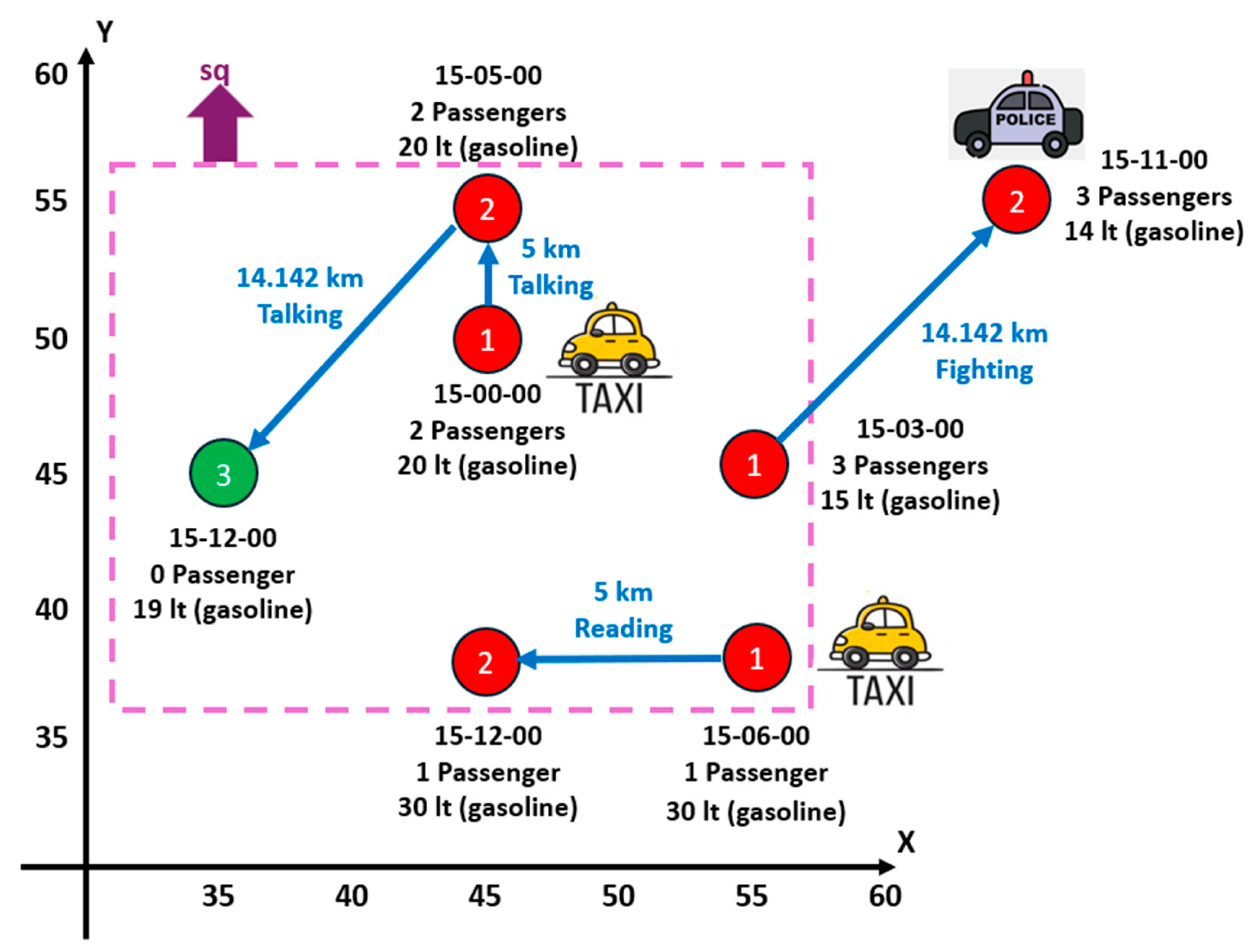
Pvalue = {pv₁, pv₂, pv₃} with pv₁ = (1, 45, 50, 25-Apr-2024:15-00-00, {true, 20, 2}), pv₂ = (2, 45, 55, 25-Apr-2024:15-05-00, {true, 20, 2}), and pv₃ = (3, 35, 45, 25-Apr-2024:15-12-00, {false, 19, 0}). In this example, the three point values have the same set of semantic attributes: SA_P = {busy, gasolineLevel, numberofPassengers}. Although our proposal allows the analyst to define point values that have different sets of semantic attributes, for simplicity, it is assumed that all the point values of the same trajectory have the same set of semantic attributes.

(ii)

Evalue = {ev₁, ev₂} with ev₁ = (1, 2, {5, “Talking”}) and ev₂ = (2, 3, {14.142, “Talking”}). In this example, the two edge values have the same set of semantic attributes: SA_E = {distance, passengersActivity}. Although the present proposal allows the analyst to define edge values that have different sets of semantic attributes, for simplicity, it is assumed that all the edge values of the same trajectory have the same set of semantic attributes.

Here, the semantic attributes of the trajectory are SA_T = {vehicleType}; thus, in this trajectory, the vehicle type is a taxi.

In Figure 3, the trajectory which might correspond, e.g., to a taxi ride, is shown.

Next, some examples of aggregate functions applied to the semantic attributes of points and edges values are presented.

(i)

For semantic attributes of points: Given that AggFnumberofPassengers = {AVG, SUM}, then AVG([2, 2, 0]) = 1.333 (note that this is the average of the number of passengers by point) and SUM([2, 2, 0]) = 4. Now, for AggFgasolineLevel = {AVG}, AVG([20, 20, 19]) = 19.666.

(ii)

For semantic attributes of edges: Given that AggFdistance = {SUM}, SUM([5, 14.142]) = 19.142. Now, for AggFpassengersActivity = {MODE}, MODE([“Talking”, “Talking”]) = “Talking”.

Here, aggregate functions to the semantic attributes of a single trajectory have been applied. However, if a set of trajectories (for simplicity, trajectories with the same semantic attributes) is given, aggregate functions to the semantic attributes of a set of trajectories can also be applied, as shown in Section 3.11. For example, if three trajectories are given, two with vehicleType = “Taxi” and one with vehicleType = “Bicycle”, and given that AggFvehicleType = {MODE}, then MODE([“Taxi”, “Taxi”, “Bicycle”]) = “Taxi”.

3.11. Aggregation of a Set of Trajectories

Consider a square region sq of the Square datatype (a sub-datatype of the Geometry datatype) of side of lenght l (Z⁺ datatype) that is traversed by a set of trajectories TRAJ (each trajectory of TRAJ is of Tdt datatype) during a time interval ti (Time Interval datatype). It is asked to find the aggregate value of TRAJ in sq during ti for a specific semantic attribute sa (whether it be a semantic attribute of a point, of an edge, or of a trajectory) and a specific aggregate function aggf that is valid to be applied to sa. That is, a function called AggregateTrajectoriesSA is given with the following prototype:

Square × PowerSet(TRAJECTORY) × Time Interval × ATTR × AGGF → DTF(aggf),

where TRAJECTORY is the set of all trajectories of the trajectory database and AGGF is the set of all aggregate functions available in the database. The aggregate function aggf ∈ AGGF must be valid to be applied to the semantic attribute sa ∈ ATTR.

Next, a pseudo-code for this function is presented. First, the pseudo-code for the semantic attribute of a point is given. AggregateTrajectoriesSAPoint (Algorithm 1) function is a special case of function AggregateTrajectoriesSA for points.

Algorithm 1. AggregateTrajectoriesSAPoint.

Function AggregateTrajectoriesSAPoint(sq, TRAJ, ti, sa, aggf)

Input: sq ∈ Square; TRAJ ∈ PowerSet(TRAJECTORY); ti ∈ Time Interval; sa ∈ ATTR;

aggf ∈ AGGF;

Output: aggvalue ∈ DTF(aggf) /* DTF(aggf) is the resulting datatype of applying aggf to a

multiset of values each of DTF(sa) */

Variables: multisetsa ∈ multiset of DTF(sa); // An array of DTF(sa) values

BEGIN

1.     IF aggf ∉AggFsa THEN /* Check if the aggf function is valid to be applied to the attribute

sa */

2.            RETURN error;

3.     END IF

4.     FOREACH trajectory Tv ∈ TRAJ LOOP

5.          FOREACH point Pv ∈ Tv LOOP

6.            IF (Pv.x, Pv.y) IS INSIDE sq AND /* Check spatial containment of the point in the                                                                              square */

7.                Pv.t ∈ ti THEN // Check temporal containment of the point in the time interval

8.                multisetsa.Add(Pv.sa); // Add value of sa to the multiset

9.             END IF

10.       END FOREACH

11. END FOREACH

12. aggvalue = aggf(multisetsa); // Apply the aggregate function aggf to the multiset

13. RETURN aggvalue;

END Function

Next, the corresponding pseudo-code for the semantic attribute of an edge is presented with function name AggregateTrajectoriesSAEdge (Algorithm 2), where a function getPoint() (lines 6, 7, and 8) is assumed, which receives a point identifier and returns the corresponding point.

Algorithm 2. AggregateTrajectoriesSAEdge.

Function AggregateTrajectoriesSAEdge(sq, TRAJ, ti, sa, aggf)

Input: sq ∈ Square; TRAJ ∈ PowerSet(TRAJECTORY); ti ∈ Time Interval; sa ∈ ATTR;

aggf ∈ AGGF;

Output: aggvalue ∈ DTF(aggf) /* DTF(aggf) is the resulting datatype of applying aggf to a                                                           multiset of values each of DTF(sa) */

Variables: multisetsa ∈ multiset of DTF(sa); // An array of DTF(sa) values

BEGIN

1.     IF aggf ∉AggFsa THEN /* Check if the aggf function is valid to be applied to the attribute                                                       sa */

2.            RETURN error;

3.     END IF

4.     FOREACH trajectory Tv ∈ TRAJ LOOP

5.          FOREACH edge Ev ∈ Tv LOOP

6.            IF (getPoint(Ev.pointId1).x, getPoint(Ev.pointId1).y) IS INSIDE sq AND

7.               (getPoint(Ev.pointId2).x, getPoint(Ev.pointId2).y) IS INSIDE sq AND /* Check spatial containment of the two points of the edge in the square. A straight line between PointId1 and PointId2 is assumed */

8.             getPoint(Ev.pointId1).t ∈ // Add value of sa to the multiset

9.           multisetsa.Add(Ev.sa); ti AND getPoint(Ev.pointId2).t THEN /* Check temporal containment of the edge in the time interval */

10.       END IF

11.       END FOREACH

12. END FOREACH

13. aggvalue = aggf(multisetsa); // Apply the aggregate function aggf to the multiset

14. RETURN aggvalue;

END Function

Next, the corresponding pseudo-code for the semantic attribute of a trajectory is presented with function name AggregateTrajectoriesSATrajectory (Algorithm 3). The value of the semantic attribute in the multiset (line 13) is included if the entire trajectory is inside (spatially and temporally, lines 6 to 11) the square (sq) and contained in the time interval (ti); however, the analyst may relax this condition, e.g., to include the value of the semantic attribute in the multiset if only a part (e.g., more than 50% of the trajectory) of the trajectory (a subtrajectory) is inside the square.

Algorithm 3. AggregateTrajectoriesSATrajectory.

Function AggregateTrajectoriesSATrajectory(sq, TRAJ, ti, sa, aggf)

Input: sq ∈ Square; TRAJ ∈ PowerSet(TRAJECTORY); ti ∈ Time Interval; sa ∈ ATTR;

aggf ∈ AGGF;

Output: aggvalue ∈ DTF(aggf) /* DTF(aggf) is the resulting datatype of applying aggf to a                                                           multiset of values each of DTF(sa) */

Variables: multisetsa ∈ multiset of DTF(sa); // An array of DTF(sa) values                             flag ∈ Boolean; // Check spatial and temporal containment of a trajectory

BEGIN

1. IF aggf ∉AggFsa THEN /* Check if the aggf function is valid to be applied to the attribute                                                       sa */

2.            RETURN error;

3.     END IF

4.     FOREACH trajectory Tv ∈ TRAJ LOOP

5.         flag = TRUE;

6.         FOREACH edge Ev ∈ Tv LOOP

7.         IF (Pv.x, Pv.y) IS NOT INSIDE sq OR/* Check spatial containment of the point in the                                                                      square */

8.                 Pv.t ∉ ti THEN // Check temporal containment of the point in the time interval

9.                 flag = FALSE;                       EXIT LOOP;

10.       END IF

11.       END FOREACH

12.       IF flag = TRUE THEN /* Check if all the points of the trajectory were inside the square                               and inside the time interval */

13.             multisetsa.Add(Tv.sa); // Add value of sa to the multiset

14.       END IF

15. END FOREACH

16. aggvalue = aggf(multisetsa); // Apply the aggregate function aggf to the multiset

17. RETURN aggvalue;

END Function

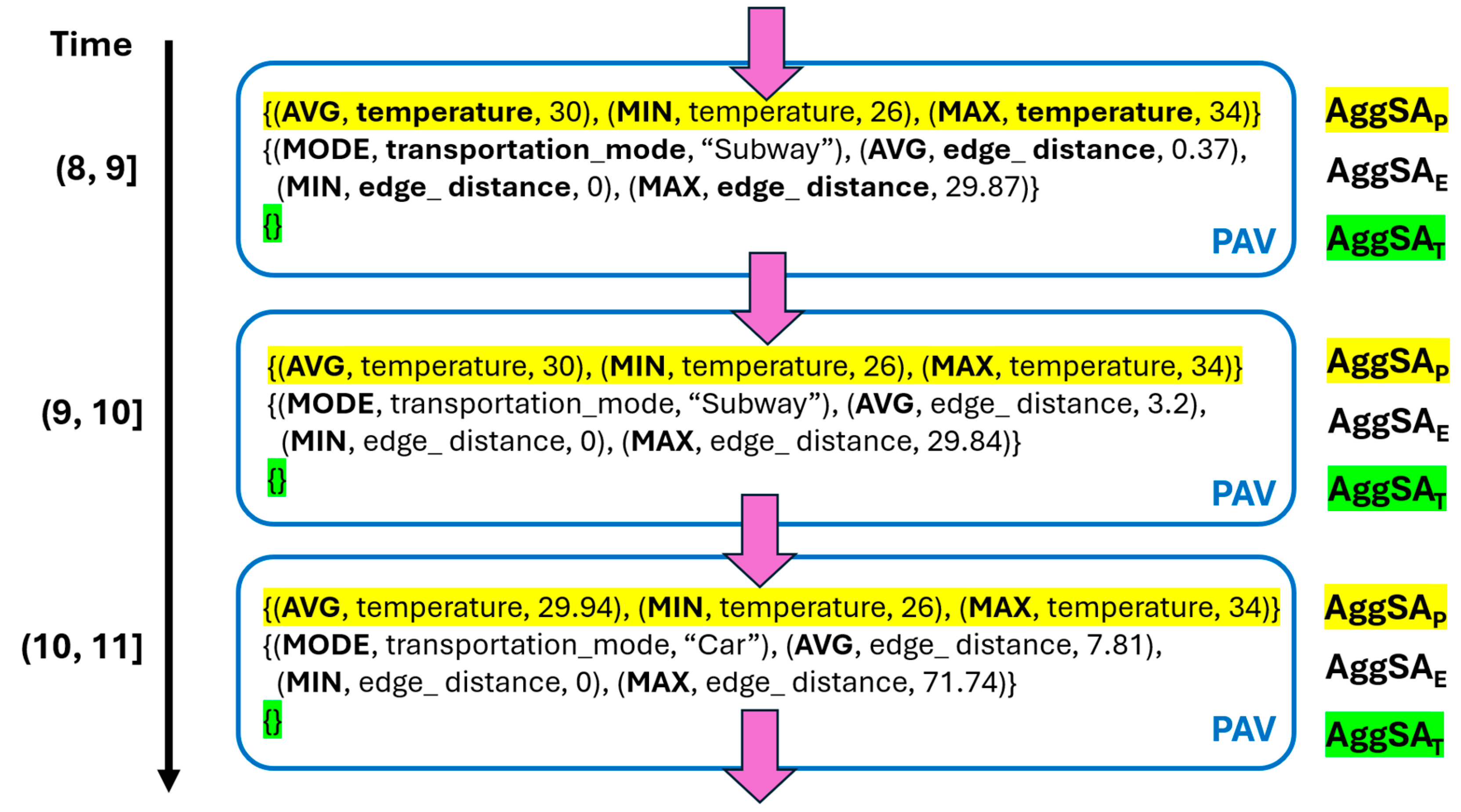
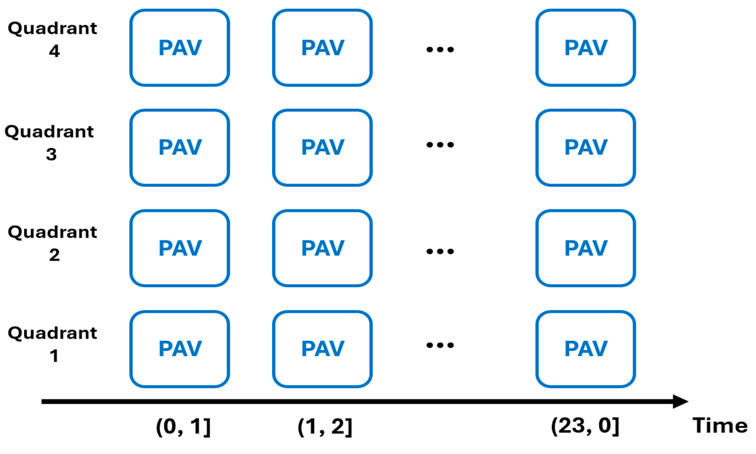
3.12. Package of Aggregate Values of a Set of Trajectories

A package of aggregate values (PAV) of a set of trajectories is defined in this subsection, as follows. Consider the previous definitions regarding a square region sq, a set of trajectories TRAJ, and a time interval ti.

Then, for each semantic attribute sa (whether it is a semantic attribute of a point, of an edge, or of a trajectory) and for each aggregate function valid to be applied to sa, the corresponding aggregate values are computed (using the corresponding functions AggregateTrajectoriesSAPoint, AggregateTrajectoriesSAEdge, and AggregateTrajectoriesSATrajectory) and create with them a PAV.

Formally, a PAV is a tuple (AggSA_P, AggSA_E, AggSA_T), where AggSA_P = {(aggf_j, sap_k, aggf_jsap_k)}, for j = 1, 2, …, Card(AggFsap_k); for k = 1, 2, …, n. That is, aggf_j is (the name of) the aggregate function, sap_k is (the name of) the semantic attribute, and aggf_jsap_k represents the aggregate value of applying the aggregate function aggf_j to the semantic attribute sap_k (this value is obtained using the AggregateTrajectoriesSAPoint function). Card(AggFsa_k) is the total number of aggregate functions that are valid to be applied to sap_k and n is the total number of semantic attributes of the point (n = Card(SA_p)).

In a similar way, AggSA_E = {(aggf_j, sae_k, aggf_jsae_k)}, for j = 1, 2, …, Card(AggFsae_k); for k = 1, 2, …, n; where n = Card(SA_E)), and AggSA_T = {(aggf_j, sap_k, aggf_jsat_k)}, for j = 1, 2, …, Card(AggFsat_k); for k = 1, 2, …, n; where n = Card(SA_T).

• Example:

Consider Figure 4, where three trajectories are shown (two trajectories of taxis and one of a police car) that occurred on a specific day, e.g., on 20 October 2024. Then, the PAV for these three trajectories (TRAJ) is calculated, where sq corresponds to the dotted violet square shown in Figure 4 and ti = [20/Oct/2024 15-00-00, 20/Oct/2024 15-30-00].

First, AggSA_P is calculated. It is given that SA_P = {busy, gasolineLevel, numberofPassengers}, AggFbusy = ø, AggFgasolineLevel = {AVG}, and AggFnumberofPassengers = {AVG, SUM}, and the following multiset of gasolineLevel values: [20, 20, 19, 30, 30, 15] (note that the gasoline level equal to 14 lt from the second point of the police car trajectory is not considered because is outside sq). Thus, AVG([20, 20, 19, 30, 30, 15]) = 22.333. The following multiset of numberofPassengers values is also given: [2, 2, 0, 1, 1, 3]. Thus, AVG([2, 2, 0, 1, 1, 3]) = 1.5 and SUM([2, 2, 0, 1, 1, 3]) = 9. Then, AggSA_P = {(AVG, gasolineLevel, 22.333), (AVG, numberofPassengers, 1.5), (SUM, numberofPassengers, 9)}.

Now, AggSA_E is calculated. It is given that SA_E = {distance, passengersActivity}, AggFdistance = {SUM}, and AggFpassengersActivity = {MODE}, and the following multiset of distance values: [5, 14.142, 5] (note that the distance of the edge of the police car trajectory is not included because it is not entirely inside sq). Thus, SUM[(5, 14.142, 5)] = 24.142. The following multiset of passengersActivity values is also given: [“Talking”, “Talking”, “Reading”]. Hence, MODE([“Talking”, “Talking”, “Reading”]) = “Talking”. Then, AggSA_E = {(SUM, distance, 24.142), (MODE, passengersActivity, “Talking”)}.

Finally, AggSA_T is calculated. SA_T = {vehicleType} and AggFvehicleType = {MODE} are given, as well as the following multiset of vehicleType values: [“Taxi”, “Taxi”] (note that the police car is not included because its trajectory is not entirely inside sq). Thus, MODE([“Taxi”, “Taxi”]) = “Taxi”. Then, AggSA_T = {(MODE, vehicleType, “Taxi”)}.

Therefore, PAV = (AggSA_P, AggSA_E, AggSA_T) = ({(AVG, gasolineLevel, 22.333), (AVG, numberofPassengers, 1.5), (SUM, numberofPassengers, 9)}, {(SUM, distance, 24.142), (MODE, passengersActivity, “Talking”)}, {(MODE, vehicleType, “Taxi”)}).

4. Experiments

For the experiments, the Microsoft Geolife GPS trajectory dataset from the Kaggle website (https://www.kaggle.com/datasets/arashnic/microsoft-geolife-gps-trajectory-dataset (accesed on 20 November 2024)) was used. The dataset corresponds to 182 trajectories, located in Beijing, China, and covers a period from April 2007 to August 2012. This dataset, which is distributed, for each trajectory, across several files, includes for each point of each trajectory the following attributes: latitude (in decimal degrees using WGS 84, a standard world geodetic system), longitude (in decimal degrees using WGS 84), altitude (in feet, this attribute is not used), date (number of days that have passed since 12-30-1899, this attribute is not used), datetime, transportation mode (airplane, bike, boat, bus, car, motorcycle, run, subway, train, and walk), and trajectory identifier (a natural number). In

Table 2. Sample from the dataset.

Latitude	Longitude	Datetime	Transportation Mode	Trajectory Identifier
39.963966	116.328324	7 November 2008 09:02:42	Bus	24
39.964004	116.328321	7 November 2008 09:02:44	Bus	24
39.964051	116.328321	7 November 2008 09:02:46	Bus	24
39.964103	116.328319	7 November 2008 09:02:48	Bus	24
40.0771166	116.3288333	21 June 2007 12:28:34	Walk	117
40.0696	116.3296666	22 June 2007 14:55:12	Train	117

, a sample of the dataset is shown.

Postgres 16 with the PostGIS 3.4 extension was also used, which is especially useful for GPS data processing, and Python 3.11.2 for loading the data into the Postgres database. The Postgres database used for the experiments includes the following tables:

Table Point: This table stores data for each point of a trajectory and includes the following attributes: (i) id, the unique identifier of the point (this attribute is generated, a consecutive integer), (ii) latitude and longitude, the geographical coordinates of the point, (iii) datetime, the date and time when the point occurred, (iv) transportation_mode, the transportation mode used at the point, (v) trajectory_id, the identifier of the trajectory to which the point belongs to, (vi) temperature, the temperature at the time when the point occurred (this attribute is generated as explained later in this section), and (vii) distance, the distance from the previous point (this attribute is also generated, as explained later in this section). The transportation_mode attribute is an edge semantic attribute; thus, if a point value pv₁ has bus as transportation mode and point value pv₂ has bike, then the edge between pv₁ and pv₂ has bus as transportation mode.

Table Trajectory: This table stores data for each trajectory and includes the following attributes: (i) id, the unique identifier of the trajectory, (ii) start_time and end_time, the time when the trajectory started and ended, (iii) total_time_seconds, the total duration (in seconds) of the trajectory, (iv) start_latitude and start_longitude, the geographical coordinates of the first point of the trajectory, (v) end_latitude and end_longitude, the geographical coordinates of the last point of the trajectory, and (vi) total_distance, the total distance (in kilometers) covered by the trajectory.

A sample of this dataset is chosen and after the load, 12 million records are obtained (i.e., trajectory points), corresponding to 69 trajectories (it took six hours of processing in an Intel Pentium CPU 6405U 2.40 GHz with 8 GB RAM). However, not all trajectories had a value in the transportation_mode attribute; therefore, after discarding the trajectories without this value, 65,000 records were retained corresponding to 29 trajectories.

Given that the dataset only had one edge semantic attribute (transportation_mode), semantic attributes of points and trajectories are also needed to check the proposal. Therefore, the 29 trajectories are enriched with additional semantic attributes. Next, the enrichment process is explained.

Data Enrichment

The following semantic attributes are included.

(i)

Semantic attribute of a point

Temperature: To generate this semantic attribute, the average temperature of the region is found (East Asia) (according to Visual Crossing, https://www.visualcrossing.com/weather-history (accessed on 2 April 2025), it was 30 °C) when the 29 trajectories occurred. Then, random temperatures for each point of each trajectory are generated, i.e., values between 26 °C and 34 °C.

(ii)

Semantic attribute of an edge

In addition to the transportation_mode attribute, the distance of each edge is included.

edge_distance: To generate this semantic attribute, the PostGIS function ST_DISTANCE is applied to calculate the Cartesian distance between two consecutive points of a trajectory, i.e., the linear distance of an edge.

(iii)

Semantic attributes of a trajectory

total_trajectory_time: To generate this semantic attribute, the time of the first point is subtracted from the time of the last point of a trajectory. This semantic attribute represents the total duration (in seconds) of the trajectory.

total_trajectory_distance: To generate this semantic attribute, the distances of all edges of a trajectory are added. This semantic attribute represents the total distance (in kilometers) covered by a trajectory.

After enriching the 29 trajectories with semantic attributes, the next step was to implement and apply the proposed algorithms AggregateTrajectoriesSAPoint, AggregateTrajectoriesSAEdge, and AggregateTrajectoriesSATrajectory. These algorithms were developed as functions in Postgres using its programming language PL/pgSQL (Procedural Language/PostgreSQL). In Appendixes A–C, the code corresponding to these three algorithms is presented with the specific implementations for computing the average (AVG) of the temperature attribute (AggregateTrajectoriesSAPoint), the mode (MODE) of the transportation_mode attribute (AggregateTrajectoriesSAEdge), and the maximum (MAX) of the total_trajectory_distance attribute (AggregateTrajectoriesSATrajectory).

For applying these algorithms, the entire region is initially considered where all the trajectories occurred. The entire region (square) is defined by the following boundaries: latitudes between 39 and 41 and longitudes between 115 and 117.

Next, the algorithms are applied in the entire region, considering a specific day, 11 September 2011. This date was chosen because it had the highest number of records, 42,847, corresponding to four trajectories. The day, 11 September 2011, is divided into 24 time intervals, i.e., an interval for each hour of the day.

For each time interval, the following aggregate values are obtained:

(i)

Mode (MODE): transportation_mode.

(ii)

Average (AVG): edge_distance, temperature, total_trajectory_time, and total_trajectory_ distance.

(iii)

Minimum (MIN): edge_distance, temperature, total_trajectory_time, and total_trajectory_ distance.

(iv)

Maximum (MAX): edge_distance, temperature, total_trajectory_time, and total_trajectory_distance.

The results are shown in

Table 3. Aggregate values for the entire region on 11 September 2011. n.d. stands for no data.

Time Interval (Hours)	MODE of Transportation_Mode	AVG Edge_ Distance (km)	MIN Edge_ Distance (km)	MAX Edge_ Distance (km)	AVG Temperature (°C)	MIN Temperature (°C)	MAX Temperature (°C)
(0–1]	Subway	2.8	0	164.87	29.95	26	33.99
(1–2]	Subway	0.79	0	118.77	29.97	26	34
(2–3]	Subway	1.07	0	118.77	29.9	26	34
(3–4]	Subway	8.57	0	71.41	30	26	34
(5–6]	Subway	1.75	0	71.41	30	26	33.99
(6–7]	Subway	0.48	0	96.9	29.99	26	34
(7–8]	Subway	0.34	0	39.66	30	26.01	33.99
(8–9]	Subway	0.37	0	29.94	29.92	26	34
(9–10]	Subway	3.2	0	29.87	29.99	26	34
(10–11]	Car	7.81	0	29.84	29.94	26	34
(11–12]	Subway	6.78	0	81.74	29.97	26	33.99
(12–13]	n.d	n.d	n.d	n.d	n.d	n.d	n.d
(13–14]	n.d	n.d	n.d	n.d	n.d	n.d	n.d
(14–15]	Walk	7.84	7.84	7.84	29.75	29.75	29.754

. Note that not all the 24 time intervals had results: this is because although the day that was chosen was the date with most records, it did not have data in all the time intervals and similarly, with the aggregate values for the semantic attributes of a trajectory, total_trajectory_distance and total_trajectory_time, since there was not a single trajectory in the four trajectories on 11 September 2011 that started and ended in the same time interval, i.e., in the same hour; therefore, the corresponding aggregate functions did not return any value (when there is no value, this is indicated in Table 3 with n.d. (no data)), because the algorithm AggregateTrajectoriesSATrajectory only considers trajectories that are entirely contained in a given time interval.

The results showed that the subway was the most used transportation mode; it was used in 10 out of the 24 intervals. In the time intervals, maximum temperatures were around 34 °C, while minimum temperatures were around 26 °C. These results are in accordance with our temperature interval [26 °C, 33 °C] for generating random temperature values. The MIN edge_distance was zero in all the intervals (except in two). This was zero when the moving object remained in the same position during two consecutive points.

Note that the proposed algorithms use all the data to calculate the aggregate values in each spatio-temporal cell, and thus, the accuracy of the results is 100% at the expense of scanning all the records. Optimization techniques, as mentioned in Section 5, are then necessary to face this challenge.

In a second experiment, the entire region is divided into four quadrants as follows. The boundaries of each quadrant are the following:

(i)

First quadrant: latitudes between 40 and 41 and longitudes between 115 and 116.

(ii)

Second quadrant: latitudes between 40 and 41 and longitudes between 116 and 117.

(iii)

Third quadrant: latitudes between 39 and 40 and longitudes between 115 and 116.

(iv)

Fourth quadrant: latitudes between 39 and 40 and longitudes between 116 and 117.

The proposed algorithms are applied to each quadrant, considering again the date, 11 September 2011, and dividing it into the same 24 time intervals that were used when the entire region was considered. The results are shown in

Table 4. Aggregate values for the first quadrant on 11 September 2011.

Time Interval (Hours)	MODE of Transportation_ Mode	AVG Edge_ Distance (km)	MIN Edge_ Distance (km)	MAX Edge_ Distance (km)	AVG Temperature (°C)	MIN Temperature (°C)	MAX Temperature (°C)
(7–8]	Walk	8.34	1.33	23.94	30.278	26.057	33.90

,

Table 5. Aggregate values for the second quadrant on 11 September 2011.

Time Interval (Hours)	MODE of Transportation_ Mode	AVG Edge_ Distance (km)	MIN Edge_ Distance (km)	MAX Edge_ Distance (km)	AVG Temperature (°C)	MIN Temperature (°C)	MAX Temperature (°C)
(0–1]	Subway	2.80	0	164.87	29.49	26	34
(1–2]	Subway	0.79	0	118.76	29.98	26	34
(2–3]	Subway	1.07	0	32.13	29.9	26	34
(3–4]	Subway	8.56	0	71.42	29.97	26	34
(5–6]	Subway	1.75	0	96.9	30.01	26	34
(6–7]	Subway	0.48	0	39.66	30	26	34
(7–8]	Subway	0.34	0	29.94	29.92	26	34
(8–9]	Subway	0.37	0	29.87	30	26	34
(9–10]	Subway	3.20	0	29.84	30	26	34
(10–11]	Car	7.81	0	71.74	29.94	26	34
(11–12]	Subway	6.78	0	78.24	29.96	26	34
(12–13]	n.d	n.d	n.d	n.d	n.d	26	34
(13–14]	n.d	n.d	n.d	n.d	n.d	26	34
(14–15]	Walk	784.69	784.69	784.69	29.75	29.75	29.75

and

Table 6. Aggregate values for the fourth quadrant on 11 September 2011.

Time Interval (Hours)	MODE of Transportation_ Mode	AVG Edge_ Distance (km)	MIN Edge_ Distance (km)	MAX Edge_ Distance (km)	AVG Temperature (°C)	MIN Temperature (°C)	MAX Temperature (°C)
(3–4]	Subway	16.55	0	33.10	30.98	29.87	32.09

. Note that for the first quadrant, there were only values (in the dataset) for the interval (7–8] and for the fourth quadrant in the interval (3, 4]. There were no results for the third quadrant (this means that on 11 September 2011, there were no trajectories that visited this quadrant).

The results show that the subway was the most frequent transportation mode, being the predominant choice in two quadrants. Maximum temperatures were around 33 °C, while minimum temperatures were around 26 °C; this was in accordance with our temperature interval. In the third quadrant, in the time intervals (12–13] and (13, 14], there were results for the aggregate values for the temperature attribute but not for the other attributes (transportation_mode and edge_distance). This means that there were no entire edges of the trajectories contained in these time intervals but there were some points contained in these time intervals.

In Figure 5, the results for the second quadrant are shown for intervals (8, 9], (9, 10], and (10, 11]. This figure allows the analyst to see the evolution of the aggregate values of a specific quadrant in different time intervals. As stated in the next section, other proposals for visualization are required to facilitate the identification of tendencies and behaviors. For example, to put several quadrants side by side in the same display to compare their aggregate values in the same or in different time intervals, see the sketch in Figure 6.

For a basic comparison, the proposed method is addressed by the presence calculation [8,9]. Indeed, the presence calculation is a special case of this proposal where the aggregate function is COUNT and the attribute to be counted is trajectory_id. Thus, the number of moving objects can be calculated in a spatio-temporal cell. When applying the AggregateTrajectoriesSAPoint algorithm, the problem of repetition counting has been tackled because each point includes trajectory_id as one of its attributes. For solving this problem, a DISTINCT clause was applied to the algorithm, i.e., SELECT COUNT(DISTINCT trajectory_id) INTO aggvalue FROM public.point. Thus, the number of different moving objects in a spatio-temporal cell is calculated.

In this experiment, the presence in each quadrant and in the entire region is calculated using the method proposed in this work where the entire day (11 September 2011) is considered as the time interval, i.e., (0, 24]. Results are shown in Figure 7.

As expected, the presence in the entire region was four; indeed, on 11 September 2011, four trajectories visited the entire region (this value corresponds to a SELECT COUNT(DISTINCT trajectory_id) of 42,847 records. Note that the presence in the third quadrant was zero because there were no trajectories that visited this quadrant.

Then, the method proposed in [8,9] was applied. Initially, a process to calculate the presence in each cell (quadrant) was run and after that, their method (distributive) to obtain the presence in the entire region was applied. For the initial process, the corresponding SQL query (it is basically the same query of the proposed method) was formulated. Next, for calculating the presence in the entire region, their method was applied and obtained: 1 + 2 + 4 = 7 (i.e., sum of the presences of the quadrants that compose the entire region). Clearly, the value is inaccurate, but keep in mind that their method generates an approximate presence value. Their method (algebraic) was also applied and obtained: for quadrants 1 and 2 (sum of their presences minus trajectories crossing their common border), 1 + 4 − 1 = 4; for quadrants 3 and 4, 0 + 4 − 0 = 4. Then, for the entire region, its presence is obtained: 4 + 4 − 1 = 7. On the other hand, the proposed method obtained the accurate value (four) at the expense of a computation that requires to count distinct trajectory identifiers in a set of 42,847 records.

5. Conclusions and Future Work

In this paper, a formal model for trajectories is proposed, as well as their semantic attributes and the corresponding aggregation operators, which can be applied to each one according to the analyst’s considerations. Semantic attributes are classified into three categories (point, edge, and trajectory attributes). The classification helps the analyst to specify the role that each attribute plays in an application. The concept of PAV is also introduced and formalized. The experiments presented in this work evidenced the feasibility of the proposal and its usefulness to discover trends and behaviors from the aggregated data of a set of trajectories occurring in a geographical region and in a time interval.

As future work, we plan to develop a visual tool that allows analysts to interactively define the schema of a trajectory, its attributes, the aggregation operators applicable to each one, load data, and visualize the results. At the end of the previous section, two possible visualizations of the results are presented that allow to analyze the spatio-temporal evolution of a set of aggregate values, i.e., of a PAV. The aggregation of complex semantic attributes (e.g., user-defined attributes, composite attributes, and multimedia attributes) is another line of research. For example, what is the average of a multiset of pictures taken by a tourist during his/her trajectory in a city?

Given that the proposed algorithms use all the data to calculate the accurate aggregate values, dealing with large trajectory datasets is a challenge. Techniques such as data sampling, calculation of approximate aggregate values, and calculation of aggregate values considering sub-aggregates values may be considered. For example, to calculate the aggregate value of a region R, considering the aggregate values of the cells that compose R, similarly as has been done in related works, to calculate the presence measure. The question posed in [2] remains open, i.e., how to obtain the aggregate trajectory (the ‘representative’ trajectory) from a set of trajectories. Our proposal is a first step towards resolving this question, since the PAVs represent the aggregate values of a set of trajectories. The next step is to associate these PAVs with a representative trajectory generated from the trajectories of the set.

References

- Spaccapietra, S.; Parent, C.; Damiani, M.L.; Fernandes de Macedo, J.A.; Porto, F.; Vangenot, C. A conceptual view on trajectories. Data. Knowl. Eng. 2008, 65, 126–146. [Google Scholar] [CrossRef]
- Oueslati, W.; Tahri, S.; Limam, H.; Akaichi, J. A systematic review on moving objects’ trajectory data and trajectory data warehouse modeling. Comput. Sci. Rev. 2023, 47, 100516. [Google Scholar] [CrossRef]
- Andrienko, G.; Andrienko, N.; Rinzivillo, S.; Nanni, M.; Pedreschi, D.; Giannotti, F. Interactive visual clustering of large collections of trajectories. In Proceedings of the 2009 IEEE Symposium on Visual Analytics Science and Technology, Atlantic City, NJ, USA, 12–13 October 2009; pp. 3–10. [Google Scholar] [CrossRef]
- Zhang, Y.; Klein, K.; Deussen, O.; Gutschlag, T.; Storandt, S. Robust visualization of trajectory data. It Inf. Technol. 2022, 64, 181–191. [Google Scholar] [CrossRef]
- Orlando, S.; Orsini, R.; Raffaeta, A.; Roncato, A.; Silvestri, C. Trajectory Data Warehouses: Design and Implementation Issues. Comput. Sci. Eng. 2007, 1, 211–232. [Google Scholar] [CrossRef]
- Meratnia, N.; de By, R.A. Aggregation and comparison of trajectories. In Proceedings of the GIS ‘02: 10th ACM International Symposium on Advances in Geographic Information Systems, McLean, VA, USA, 8–9 November 2002; pp. 49–54. [Google Scholar] [CrossRef]
- Braz, F.; Orlando, S.; Orsini, R.; Raffaeta, A.; Roncato, A.; Silvestri, C. Approximate Aggregations in Trajectory Data Warehouses. In Proceedings of the IEEE 23rd International Conference on Data Engineering Workshop (ICDEW), Istanbul, Turkey, 17 April 2007; pp. 536–545. [Google Scholar] [CrossRef]
- Baltzer, O.; Dehne, F.; Hambrusch, S.E.; Rau-Chaplin, A. OLAP for Trajectories. In Proceedings of the 19th International Workshop on Database and Expert Systems Applications, DEXA 2008, Turin, Italy, 1–5 September 2008. [Google Scholar]
- Baltzer, O.; Dehne, F.; Hambrusch, S.; Rau-Chaplin, A. Olap for Trajectories; Technical Report TR-08-11; School of Computer Science, Carleton University: Ottawa, ON, Canada, 2008; Available online: https://carleton.ca/scs/wp-content/uploads/TR-08-11-Dehne.pdf (accessed on 30 September 2024).
- Feng, J.; Shi, Y.Q.; Tang, Z.X.; Rui, C.H. Aggregation index technique of moving objects in road networks. J. Jilin Univ. (Eng. Technol. Ed.) 2014, 44, 1799–1805. [Google Scholar]
- Shi, Y.Q. A Study on the Complete Temporal Probabilistic Aggregate Query Over Moving Objects on Road Networks. Ph.D. Thesis, Hohai University, Nanjing, China, 2015. [Google Scholar]
- Shi, Y.; Huang, S.; Zheng, C.; Ji, H. A Hybrid Aggregate Index Method for Trajectory Data. Math. Probl. Eng. 2019, 2019, 1784864. [Google Scholar] [CrossRef]
- Buchin, K.; Driemel, A.; van de L’Isle, N.; Nusser, A. Center-based clustering of trajectories. In Proceedings of the 27th ACM SIGSPATIAL International Conference on Advances in Geographic Information Systems, Chicago, IL, USA, 5 November–8 December 2019; pp. 496–499. [Google Scholar]
- Aronov, B.; Har-Peled, S.; Knauer, C.; Wang, Y.; Wenk, C. Fréchet distance for curves, revisited. In Algorithms—ESA 2006; Lecture Notes in Computer Science; Springer: Berlin/Heidelberg, Germany, 2006; Volume 4168, pp. 52–63. [Google Scholar]
- Brankovic, M.; Buchin, K.; Klaren, K.; Nusser, A.; Popov, A.; Wong, S. (k, l)-medians clustering of trajectories using continuous dynamic time warping. In Proceedings of the SIGSPATIAL ‘20: 28th International Conference on Advances in Geographic Information Systems, Seattle, WA, USA, 3–6 November 2020; pp. 99–110. [Google Scholar]
- Ghazi, B.; Kamal, N.; Kumar, R.; Manurangsi, P.; Zhang, A. Private Aggregation of Trajectories. Proc. Priv. Enhancing Technol. 2022, 2022, 626–644. [Google Scholar] [CrossRef]
- Duong, T. Using iterated local alignment to aggregate trajectory data into a traffic flow map. arXiv 2024, arXiv:2406.17500. [Google Scholar]
- Tong, A.; Sharma, A.; Veer, S.; Pavone, M.; Yang, H. Online Aggregation of Trajectory Predictors. arXiv 2025, arXiv:2502.07178. [Google Scholar]
- Gómez, L.I.; Kuijpers, B.; Vaisman, A.A. Analytical queries on semantic trajectories using graph databases. Trans. GIS 2019, 23, 1078–1101. [Google Scholar] [CrossRef]