Abstract
A vital area of AI is the ability of a model to recognise the limits of its knowledge and flag when presented with something unclassifiable instead of making incorrect predictions. It has often been claimed that probabilistic networks, particularly Bayesian neural networks, are unsuited to this problem due to unknown data, meaning that the denominator in Bayes’ equation would be incalculable. This study challenges this view, approaching the task as a blended problem, by considering unknowns to be highly corrupted data, and creating adequate working spaces and generalizations. The core of this method lies in structuring the network in such a manner as to target the high and low confidence levels of the predictions. Instead of simply adjusting for low confidence, developing a consistent gap in the confidence in class predictions between known image types and unseen, unclassifiable data new datapoints can be accurately identified and unknown inputs flagged accordingly through averaged thresholding. In this way, the model is also self-reflecting, using the uncertainties for all data rather than just the unknown subsections in order to determine the limits of its knowledge. The results show that these models are capable of strong performance on a variety of image datasets, with levels of accuracy, recall, and prediction gap consistency across a range of openness levels similar to those achieved using traditional methods.
1. Introduction
It is essential for an AI system to be able to return outputs, suggesting that it has reached the limits of its classification abilities rather than returning incorrect or closely related predictions. While significant research continues to be performed into related problems under a variety of interlinking areas, including Open Set Recognition [1], Out-Of-Distribution (OOD) [2], and anomaly detection [3], these do not always address the idea of an AI system recognising what its classification limitations are, nor do they all provide models that offer both useful classification for known data while also flagging new unknowns consistently [1,4]. There are several methods that have been used previously to approach the problem with varying levels of success and usability, but most networks have been trialled on corrupted known data or solely to investigate the varying probabilities in these predictions rather than using the uncertainties to map out the model’s approach and limitations [5,6,7]. This means that the models were working in a differently defined space than what is proposed here. There is a significant body of work on this problem area, but there are so many approaches, training methods, and specific goals that wider-ranging and adaptable solutions are not necessarily at the forefront. Here, a model capable of such a task is coined as an agnostophilic network that can thrive with unknowns, as opposed to those mired in difficulties processing the unclassifiable.
Models with the mixed abilities described above would have multiple applications across many industries, especially those where both incorrect predictions and unknown data are frequent and damaging; medicine and cyber security, for example, are constantly pushing these challenges. Successful and useful models here would result in less need for human intervention and checks, leading to more efficient systems without increasing risk. Building on previous work using probabilistic techniques could expand the capabilities of what has been proven and develop more utility while also providing a path to further investigate the underlying nature of probabilistic classifiers, how they evaluate data and consider the options before them when applying predictions for insight into the improving intelligence of AI. The distributions delivered by Bayesian Neural Networks (BNNs) offered a promising avenue of exploration with regard to the inner working of a model as it is presented with such a problem.
Neural Network classifiers are notoriously overconfident, frequently offering 90% probabilities on incorrect predictions [8]; it is therefore vital to temper this characteristic. A traditional or deterministic neural network functions through the use of weights, outputting a probability of its prediction through the final SoftMax layer [9]. Because one of the SoftMax outputs is the probability that a datapoint belongs to a particular class, an obvious strategy would appear to be to assign a cut-off point at which this probability is too low, and the model is uncertain, as, at first, it seems that a high probability would tend towards an accurate prediction. However, the unearned overconfidence prohibits this. A Probabilistic Neural Network (PNN), which replaces the SoftMax layer with a probabilistic one, demonstrates less confident predictions over the label options. For this type of model, the loss function—or the difference between the target values and the model output—is the negative log-likelihood of each target sample given the predicted distribution. The network output is therefore a distribution rather than a determination. BNNs use distributions for the network weights, which are learned through Bayesian inference. This accounts for the epistemic uncertainty, or the systematic lack of knowledge of the model and process and provides insightful distributions in the output through which the model’s consideration of individual datapoints can be observed. Due to the assumption that Bayesian methods cannot work properly with unknown data, the concept of using BNNs for this type of problem has been under-explored. In this work, we demonstrate that the approach offers significant advantages to the field, particularly when it comes to maintaining model performance across varying levels of dataset openness and the potential for use outside of computer vision and image identification. The ability to explore distributions of predictions in a user-friendly manner through probability plots also enhances both wider understanding of the model and network tuning capabilities in a way that non-Bayesian models do not.
In this paper, we explore this solution through creating a BNN capable of a clear and consistent difference between the probability levels in predictions for previously seen and previously unseen data such that it then flags data that the model did not recognise as any familiar class. The difference between the model’s confidence in control data predictions and in unseen data predictions is a vital goal for a useful model. For example, a known data confidence of 0.85 and an unseen confidence of 0.65 gives a difference of 0.2, which is significant enough to determine where the model’s knowledge fails; this is henceforth referred to as the confidence delta. By tuning a BNN to have strong recall and certainty levels on known or control data, as well as low confidence in predictions for unknowns, the confidence delta could be further widened and then used as a benchmark for determining whether or not data was recognized and classifiable by the model, or whether the data was too anomalous within what had been learned previously. This approach holds several challenges, as custom metrics would be required, and the accuracy for control data at the point that the network still functions as a useful classifier. Even when the overconfidence is regulated, many neural networks struggle with generalization. Adjusting hyperparameters with the goal of increasing model confidence for knowns and decreasing it for unknowns is a new area, so numerous experiments and manual network architectures would be necessary. In order to achieve this, mixed image datasets were built with certain select numbers chosen as the control classes. Initial networks were trained and tested on these to achieve a baseline model before being tested on previously unseen images. The use of BNNs allowed for the examination of probability distributions, which could then be used to aid custom tuning. Experiments focused on network architecture, different image sets, volumes of data, and model parameters until an optimal configuration was found. It was discovered that, with the correct structuring and training, clear and consistent differences between the confidence levels for control and unknown data could be returned, allowing for the accurate classification of “knowns” and the identification of anomalous or unknown datapoints. A usable model capable of recognizing both classifiable data and the limits of its own knowledge can be built for image data and can likely be expanded significantly for use in other areas.
The rest of this paper is organized as follows: Section 2 describes the relevant current literature and gives a brief background into Bayesian Neural Networks. Section 3 describes the creation of the datasets and the experiments performed in building and testing the initial networks. The experimental results are shown in Section 4, with explanations as to the problems that arose during the work and the methodological approaches that lead to their solutions. The best performing model is detailed in Section 4.3, and its results are presented and explained. Finally, Section 5 concludes the paper and discusses further potential work in this area.
2. Background and Previous Literature
There is a wealth of previous work in the combined elements that make up this work: image classification, anomaly detection, probabilistic modelling, and Open Set Recognition have been increasingly explored in recent years, with the identification of an unclassifiable datapoint a particularly varied area of study in terms of ideas and methods [10,11]. With growing sophistication in modelling types and the availability and accessibility of large data, models can be built that excel in the classification or prediction problem that they are specifically designed for but may still struggle with unexpected inputs. This leads to trade-off considerations between using an otherwise successful model or developing further to account for a handful of errors depending on how significantly they could affect wider outcomes. There is no obvious and immediate path to solutions and no guarantee that one approach will work for all data types and industry environments. Within the wide area of anomalous data identification, it is worth considering two types of problem: classification with rejection (CWR), and Open Set Recognition (OSR) [1]. The former concentrates strictly on training and testing with known classes and, during testing, rejecting those that it is uncertain about based on confidence levels or some other criteria. It does not work to highlight the unknown specifically, nor is it applicable to complete unknowns, working under a closed-set assumption. While the title of OSR continues to be used for a number of similar tasks, it is generally considered to consist of classifying known or control classes while rejecting unknown and previously unseen ones. The distinction is important as it limits the methods and algorithms that can be used, particularly in terms of probability models.
The CWR concept is decades old with many methods such as SVMs successfully tested [12,13], but trials using Deep Neural Networks are more recent, with early explorations detailed in “Selective Classification for Deep Neural Networks” [14]. The study has a strong focus on risk control and the trade-off between this and the cost of errors. It uses the SoftMax response method, applying a pre-selected threshold on the maximal neuronal response of the layer. While not unsuccessful, the overconfidence inherent to NNs [8] is a clear limitation of this approach, with the model still confidently giving incorrect results. Another approach to this problem is probabilistic modelling, which can better analyze network confidence problems. With increases in this type of study and more off-the-shelf methods available, BNNs can now be built using TensorFlow packages when custom functions are built for the posterior weight distributions. This type of exploration has become popular on the corrupted MNIST set, a version of the classic MNIST (Modified National Institute of Standards and Technology database) set of handwritten figures with intentional noise over the images to confuse a model [5,15]. While they have a place in OSR research, corrupted or unknown data are also a potential question of data quality; a model may be unintentionally misled by an input that is of low quality, particularly in the computer vision field. When considering the manner in which most AI approaches break down the classification problem and the way the assumed quality of imagery has increased substantially, it may not be the case that significant noise is expected in modern test data. However, images are often compressed or otherwise processed in ways leading to a decrease in quality that could be considered to verge on corruption. Different types of quality-distorted images were presented to transformer classification networks in order to examine the effect on performance [16]. While compressed images did not cause great issue, those with various Gaussian noise applied caused decreases in accuracy, with the study suggesting that model robustness should be enhanced in the training phase by considering noise augmentation techniques. A significant and detailed example demonstrating the differences between the aleatoric and epistemic uncertainties was produced by research engineer Chanseok Kang in 2021 [17], and this work informs the early parts of our study. The network provides low confidence predictions when presented with an image unrecognizable due to the image being partially covered or otherwise manipulated. Work using BNNs to highlight the “I don’t know” possibilities of the method on image sets stops when the probability distributions for corrupt data are achieved, and there is little progress towards a clear and useful gap in confidence levels.
OSR attempts to classify known or control classes and reject or group unknowns into a new class or classes via decision boundaries [1]. This allows for the unknown classes to be set aside rather than incorrectly classified into a useful group. The concept of the openness of the data is the subject of many discussions in the area [18], defined as follows:
where
= Number of classes in the training set.
= Number of all existing classes.
= Number of targeted classes.
OSR is often seen as an extension of classification, and, as Neural Networks (NNs) have proven to be particularly strong classifiers, there have been many attempts at using them for this task. As mentioned, however, NNs, including Deep Neural Networks (DNNs) tend to be overconfident and therefore easily fooled by new or corrupted data [11]. This is due to the SoftMax cross-entropy classification loss, which also serves to give NNs a closed-set nature. A frequently used method of combating this is altering the final layer type. Using an OpenMax layer instead and using a mean activation technique was successful in recognizing unknowns but failed to work well enough on adversarial images more closely related to training samples [19].
Another end-layer method used a competitive overcomplete output layer (COOL), which assigned more than one output per class in order for the outputs to compete to achieve the accurate result [20]. Still using the 0.5 threshold value, this gave the model options to consider and reject unknowns more thoroughly; fake samples generated to fool the model had to be much more complex to result in an incorrect classification than those generated for testing a normal COVNET architecture using the MNIST dataset. Single-class experiments reached accuracy/correct rejection rates of 0.8, with multiclass on the CIFAR dataset reaching 0.75. As both datasets were also used in this study, it makes for a useful comparison regarding OSR as a computer vision problem. The model in this study was able to approach 0.85 accuracy with the CIFAR set as a multiclass task. The paper suggests that NN fooling is more a problem of datasets rather than the models used for the task, as each will have unique inter-and intra-spacing. This is a convincing idea, both in terms of the spatial theory behind it and the variability of results when applying previously successful model approaches to different data types.
Another recent approach attempting to build a deep learning network for OSSR with focus on strongly handling unknown unknowns mathematically modelled the distance metric between class spaces in terms of Wasserstein distance as opposed to the Euclidean distance typically employed in these scenarios [21]. This is of particular note as explorations of the effect and methods of class-space distance continue to drive work in this field as the measurements are used to correlate similarities in the data [22]. The algorithm is made up of three sub-modules, with the other two consisting of class-space compression and a vision transformer-based signal representation. When applied to electromagnetic time-series data, improvement was demonstrated compared to methods such as OpenMax, particularly with mobile phone signal data.
A different approach noted the strength of neural networks as classifiers and the potential issues extending them for OSR, offering instead a weightless neural network (WiSARD) as a solution [18]. The model used complex distance-type methods with the rejection thresholds defined during the training period. Where normal NNs have weights attached to the edges connecting nodes, the connections here have no weights at all, making the nodes the source of learning. The network discriminators store knowledge on classes and on the multiple-threshold rejection technique, rating the observations according to the qualifying features rather than using prior data distributions. The concept of the “openness” and the closely related “coverage” of training and testing data is thoroughly explored, with multiple class experiments taking place using the UCI-HAR dataset, a multivariate timeseries of simple human activities. Mainly using an “odd-one-out” approach of training on five of the activities and testing with all six, the model achieved reasonable F1-macro scores, particularly when compared to other algorithms such as SVMs. While this represents a different datatype than the image data used in this study, the highest performance in the results falls short of that achieved with the BNN method, even with custom manual thresholding. Further experiments focused on increasing openness, and, here, the model struggled with recall, reaching under 0.7. This was true of the compared methods tried for the same task, which included Gaussian Naïve Bayes, a more basic NN, and an SVM. As the weightless network and the SVM, both methods that only use the training data, performed the best, the study suggested that information regarding additional classes may simply serve to mislead models and decrease OSR performance.
A further publication of note is “Reducing Network Agnostophobia” [23], which explored the question of identifying unknown unknowns, detailing drawbacks of previous methods including the SoftMax threshold and the background class approach. It noted that a novel loss function improved performance in terms of identifying new unknowns, comparing a more probabilistic approach to that of specific background training classes. The special metrics used, however, are not comparable to this work. There is a dearth of probabilistic models attempting to solve the OSR problem, and this is largely due to the assumption that the underlying law of total probability cannot properly translate to the issue of previously unseen data [20,24]. Probabilistic models also tend to use the maximum a posteriori probability (MAP) estimate, which requires the full posterior distribution; this is not accessible with unknown unknowns, and the known classes have been so far considered insufficient for the task. Instead, some experiments have used a Compact Abating Probability (CAP) method, in which the probability of class falls during the move from known data to open space. Replacing the need for unknowns to be modelled, this SVM technique was trialled on several datasets with varying degrees of openness. While successful in recognizing unknowns, the results demonstrate a similar issue with increasing openness as the previously mentioned DNN studies, that is, a decrease in F1 scores. The more “open” the sets, the lower performance tends to be, whatever the algorithm. The high F1 scores of the best model at lower openness fall significantly to 0.86 as openness approaches 14% when experiments used the LETTER dataset. While scores between 0 and 12% openness stay above 0.9, they fare better in the results from MNIST experiments where they remain over 0.9 at the highest level (13%). The experiments performed in the SVM study focus on these grayscale image sets, comparing them against dropped out images within the set. The study described in this paper uses the MNIST and FMNIST sets for grayscale image experiments, both on their own and mixed together, as well as mixes of colour image CIFAR sets. This allows for both wider and narrow similarities in the training and testing data, as well as more varied coverage; openness beyond 14% was frequently trialled, with scores remaining 0.85+. The method used may be less susceptible to the openness problem than the SVM probability or the weightless neural network approaches.
The uncertainty of predictions was a key feature of an OSR method for malware traffic recognition, aiming to create a network capable of identifying unknown and unseen attacks [7]. The Deep Evidence Malware Traffic Recognition (DEMTR) achieved high F1 scores for known and unknown test data. However, these decline quickly with increasing dataset openness, an issue that remains a significant challenge in this field. While there is some comparison with the use of Bayesian probability distribution methods in classification, the underlying issues of the incalculable denominator are not addressed as the comparison investigates the method of reaching the certainty estimate rather than the performance regarding unknown inputs. The study does indicate that there is room for considering probabilistic approaches to the OSR problem.
A recent OSR technique with Gated Recurrent Unit and Convolution Auto-Encoder (GRU-CAE) deep learning networks uses a template matching method to determine a threshold: focused on classifying ocean vessel types from sound wave data, the study establishes a template for each known data type, and then the Euclidean distances in the test data are measured [25]. The template is then not a sample but an optimal vector. The results show a particularly promising approach, which, like this study, is built around novel thresholding techniques. A somewhat similar approach was used to develop a model for nuclear power plant fault diagnosis; following feature extraction through Convolutional Prototype Learning (CPL), an SVM and Prototype Matching by Distance (PMD) method determines the open space fault diagnoses [26]. Due to the nature of power plant operations, the data here is particularly complex, with multiple variables to be considered that challenge the feature extraction process. With the CPL compressing the intra-classes and separating the inter-classes, the way is paved for known faults to be identified and unknowns rejected. High accuracy was achieved for known faults, with predictably lower scores for unknowns yet still in the ~0.9 range for the best experiments.
Another technique, this time applied to image data for classifying wild fish, uses a fusion activation pattern of SoftMax and OpenMax functions for the thresholding. The former performs a preliminary screen with the latter working to perform corrections in the activation vector [27]. The WildFishNet trained on thousands of images split into hundreds of classes, with more kept back for testing as unknown data for openness levels of up to 20%. The method achieved strong results with 0.8+ accuracies across the final experiments. The dataset used, however, contains many images that are extremely similar, leading to the type of image confusion common to this type of problem. Ultimately, significant work in the OSR field is focused on the determination of a threshold from a sampled or generated ideal, often comparing new data through mathematical distances. The BNN method of extracting unknowns has so far been overlooked.
This paper challenges the notion that probabilistic, specifically Bayesian approaches, are always unsuited for the task at hand without complex adjustments. Bayesian networks have been used as powerful tools both alone and as combination models for a variety of problems as their transparency and architecture allows for the consideration of multiple factors and continuously updated knowledge in training and later application. An example of this is a hybrid model for mental health diagnosis, which combines the aforementioned strengths with Large Language Models to simulate the back-and-forth approach used in pinpointing these specific medial issues [28]. A Bayesian Neural Network differs significantly from a normal deterministic one, using distributions as weights. This special weights configuration gives BNNs the ability to better generalize as they can avoid the unnecessary extrapolation of the training data through estimation of the posterior distribution. This is achieved through Bayesian inference, using Bayes’ Rule where distribution judgements are altered in light of new data; the posterior parameter distribution is found by Equation (2):
where is the data likelihood or the probability of a particular set of data being observed under particular parameters. is the prior distribution, or the assumed distribution before further information is acquired. is the new evidence data, or new observations used to update the probability distribution. The predictions then follow as an expectation of the output over the optimized posterior distribution. In this case, the integral in Bayes’ Theorem is intractable and must be estimated through variational inference, a method by which a complex distribution is approximated from a family of densities best representing the output. This results in the model assigning a certainty value along with a standard deviation level of confidence to the predictions [29]. The uncertainty can be observed for the model as a whole or for single observations, allowing for particularly useful insights into the model’s workings and the conclusions it comes to. A further focus of this research is the levels of uncertainty for known and unknown data and the potential uses these outputs can lead to.
To implement Bayes’ Theorem in this study, the model trialled exercises spike-and-slab regression as the custom prior, which uses a prior distribution with a point mass at zero; this generally leads to a sparse posterior distribution. This method suits instances in which potential predictors outnumber the observations [30]. In terms of network architecture, this makes up the Dense Variational layer; this in turn provides control over the weight space that the model operates in due to the need to define the standard deviations for the distribution. As the distribution is a weighted sum of the two normal distributions, a higher standard deviation increases the likelihood of values away from the zero point. Due to the nature of the experiments and variation in the testing data, a more generous space is desirable. After the first rounds of training, Bayesian inference is performed to return the initial posterior distributions, or the term. Further training then continues drawing from these distribution samples, continuously updating and tuning over the model performance. Bayesian inference therefore gives the probability—or certainty—the model has regarding its predictions, and it is from here that the core of the method stems. Strong confidence on known data and low confidence on unknown data allows for the confidence delta to be created and used to determine the classifications.
As mentioned, previous work has raised the issue of unknown unknowns prohibiting the use of the above equation in OSR models as conditioning cannot be performed on all the classes, leaving the equation denominator incalculable. However, by approaching the task as a blended CWR/OSR problem, allowing the network to assume that unknowns can be treated as corrupted data, designing the architecture such that the working space is great enough, and the generalization wide enough, the resulting confidence delta between control and unknown data can achieve strong rejection levels through averaged thresholding. The model can therefore correctly classify multiple known classes while actively finding and rejecting data which does not fit. As almost all current OSR methods use a threshold-based approach, its selection depends on model knowledge from the known training data [1]. This is risky as there is obviously no supporting knowledge from the unknowns. A BNN can move this forward as it can deal with the aleatoric uncertainty inherent in the problem [31] and return information on specific troublesome observations.
3. Methodology and Metrics
To test the theory laid out in the previous sections, PNNs and BNNs for image classification were built in Python 3.7 using TensorFlow 2.1.0 and tuned for accuracy and consistent probabilities with known unknowns to serve as the base level network. Results were plotted with Matplotlib 3.5 or exported to MS Excel 2503 for clearer bar chart visuals.
The experiments required custom datasets with varying degrees of openness, complexity, and image types. Several available image sets were used, including MNIST, FMNIST, K49-MNIST, and CIFAR-10. These provided a range of images of alpha-numeric characters, Japanese characters, and images of animals and objects in various colours. Training and validation datasets were created with different numbers of classes. For example, in the case of the initial CIFAR-10 dataset, seven out of the ten image classes were extracted to create the training and validation sets. The test set was then a mix of the training and the remaining three classes, providing seven “control” and three “unknown” classes. Due to the use of one-hot encoding, the unknown classes were relabeled to replace those swapped out from the training set. Different ratios were explored, and care was taken to include and exclude images with high similarities to each other for the model to be thoroughly challenged. To increase volume and variety, some sets were mixed prior to the control and unknown classes being determined and extracted.
Once trained with the training sets, the model was given a test set consisting of both known unknowns and unknown unknowns and the results analyzed. While key metrics were strong accuracy for the control classes, high recall, and F1 scores, the main goal was a significant difference in probability levels between the control and unknown classes to determine a proper threshold for rejecting a datapoint. After tests were run, the average probability of predictions per class was collected and visualized in order to review this, with insignificant deltas indicating that the model was not yet performing successfully. Where this was the case, the results were investigated further in terms of probability distribution and epistemic uncertainties for specific datapoints, system entropy, and image confusion.
This is where the BNN method uniquely lends itself to this type of interpretation and tuning; where specific datapoints appear to be causing confusion for the model, those with frequently predicted labels alongside high uncertainty can be retrieved and the epistemic uncertainty distributions for the specific label viewed. This can also pull the images themselves for additional comparison and verification from a human perspective. Once issues have been realized, further tuning can take place with a focus on the area of confusion as opposed to simply the overall network.
This was then used as feedback to tune the model further, reconfiguring its architecture and operations to progress towards the best working network. As the main metric of the confidence delta was custom, automated tuning was not useful in this research work, and the majority of the network architecture was constructed through bespoke layering as opposed to solely off the shelf functions. Different layer types and orders were experimented with, as well as optimizers, activation functions, training epochs, and normalization methods such as batch normalization and the inclusion of dropout layers in order to arrive at the optimal design for the metrics described through minimizing overfitting and controlling loss and validation accuracies. To appraise the network configurations, the total accuracy and the recall values for both control and unknown test data were collected; it was desirable that they were consistently high for the former and low for the latter, as there would be no correct predicted value for the unknowns. Ultimately, there were two significant tuning goals involved in this method once an initial baseline model focusing simply on recall for the control data: image confusion tests and maximizing the probability delta. To achieve these, experiments were run covering various selections of
- Single-image datasets.
- Mixed-image datasets.
- Layer numbers.
- Optimizers.
- Activation functions.
- Normalization methods.
- Training epochs.
The pathway can be seen in Scheme 1.
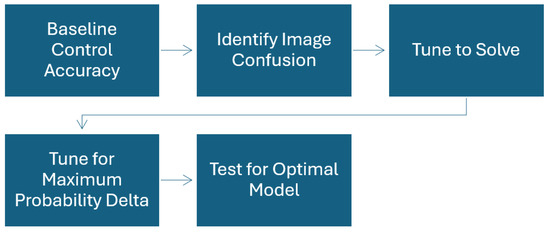
Scheme 1.
Methodology process.
4. Results
4.1. Image Confusion
As previously mentioned, the BNN method provides a unique method to investigate and solve image confusion, which is often a key component to both control and unknown classes having mixed probability results. This initial indication of the problem is sparked by the type of result seen in Figure 1, which shows the probability results of an early model for nine classes, of which one of them (0) was an unknown. The confidence level of the unknown (red) is low, which is desirable, but so is that of labels 6 and 7 to the point where there is not a useful threshold to progress with. The model here has not reached a point at which a significant confidence delta is achieved, but it provides a starting point for distribution investigation and tuning. The issue was isolated to examine the epistemic uncertainty.
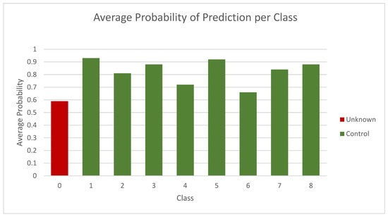
Figure 1.
Average probabilities for known (green) and unknown (red) classes for MNIST/FMNIST experiment.
The model struggles to differentiate between the figure “5” from the MNIST set and the sandal images from the FMIST set. A classic CNN could be trained to separate these fairly easily, but, when one is a complete unknown and the probability level is an essential metric, the task is more complex. When checked visually, both have similar line shapes and a large amount of negative space, both surrounding the shape and encircled within the lines as can be observed in Figure 2. This set of images was taken from the samples that the network was attempting to identify, i.e., the source of image confusion.
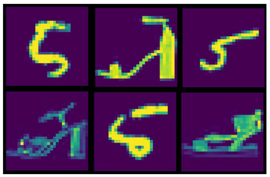
Figure 2.
Examples of the figure “5” and sandal images from the MNIST and FMNIST datasets.
For the lower confidence level predictions, i.e., under 50%, the label predicted was collected and visualized to see if there was a specific value that was being incorrectly assigned to a certain section of the data. This indicates if there were patterns to the inaccuracy or widely spread confusion. In the graph in Figure 3, the uncertain prediction is overwhelmingly the label “5”, which, in this instance, was the model attempting to classify the previously seen sandal image. This then confirmed the pattern of confusion in the model, allowing for targeted improvements in the tuning.
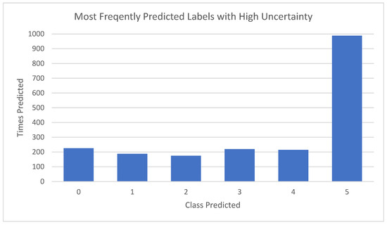
Figure 3.
Counts of predicted labels for a low confidence prediction.
Looking into the specifics, this way allows for closer investigation of not only particular images, often showing that there would be a mix of confidence levels, but also the effects of wider network alterations on predictions. For the distribution visuals, plotting code was adapted from a previous demonstration [17]. Figure 4 shows what the model estimated the labels to be for a “5” image where the sandal image had been assigned the label of 0.
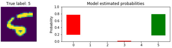
Figure 4.
Distributed predicted label probabilities showing model confusion. The red and green bars are incorrect and correct classifications respectively.
The epistemic uncertainties are represented by the stretch of the coloured bars, indicating the level of “consideration” given to the classification options available. The red bar, for instance, shows considerations between 20 and 76%. The long bars show that labels 0 and 5 gave the model significant pause. Both also have high probabilities assigned to them, as well as low. The Bayesian network allowed for this uncertainty to be visualized to determine that both the accuracy and confidence levels are too easily swayed at this stage for these datapoints; tuning while revisiting these graph types indicated the movement towards the metric ideals. From here, the network architecture was reworked and retested to account for this feedback, and fixing this level of confusion resulted in improved performance for dissimilar images as well. Layer configuration was found to have the most impactful changes. This clearly demonstrates how a BNN offers significant options for investigation and adaptation compared to other models used for open-set problems.
4.2. Maximising Probability Delta
Altering the model optimiser did not make any significant changes to any of the results, so layer structure was investigated along with the inclusion of dropout layers. Dropout layers prevent overfitting by randomly dropping a ratio of the units, providing a level of regularisation. This also assisted with the creeping overfitting inherent to this type of modelling. A notable occurrence during these trials was the effect of using such a dropout layer compared to employing batch normalisation in the network architecture. The dropout approach results in largely consistent confidence levels for both control and unknown data. Batch normalisation, however, led to unpredictable confidence levels all round and no clear pattern between control and unknowns. It is possible that the action of the dropout layer to prevent overfitting reduces confidence in the unseen images, as the random data exclusions give the model less to work with for the mixed unknowns. This is an idea that could be researched further.
It can be seen in Figure 5 that the inclusion of a dropout layer had a significant effect on the confidence delta; the addition of this to any number of layers greatly increased the difference between the known and unknown confidence levels, sometimes by several percentage points. When this phenomenon was further investigated down to the individual figures, it was discovered that the dropout layer results in a very slight confidence drop for the control data but a far more significant drop for the unknowns (1–3% and 7–8%). This resulted in a greater overall confidence delta for networks built with dropout configurations. The number of layers also demonstrates a gently rising trend, peaking at seven. The base data show that the increase in the difference comes from lower probability levels in the unseen classes, while the levels for control stay similar. The dropout approach is therefore decreasing unearned overconfidence in the model, an effect that may be worthy of further study. The seven-layer dropout configuration also had strong performance for accuracy and recall and so was used throughout this study. This optimal configuration proved true for both probabilistic and Bayesian model types, possibly due to the effects on aleatoric uncertainty.
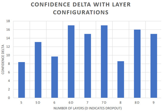
Figure 5.
Effect of layers and dropout on confidence delta.
As the changes were made, the lower and confused probabilities, as well as some of the individual datapoints, continued to be plotted to test the effects of the changes on the different uncertainty types. Figure 6 shows one such investigation when the ideal configuration had been neared; the previously unseen “5” was given to a model that had been trained on a set that included the F-MNIST sandal image. This time, little consideration was given to any of the labels, and there was low confidence in those selected. While the sandal label (5) was one of the ones predicted, the epistemic uncertainty is considerably lower with the probabilities just reaching 0.5. The small distributions and lack of wide class considerations indicate that the network was no longer confused by the unknown data and would assign low-level predictions rather than overconfident incorrect ones.
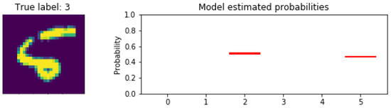
Figure 6.
Distributed predicted label probabilities showing reduced model confusion. The red bars indicate incorrect classifications.
Figure 7 and Figure 8 show the developing accuracy and recall for different layer configurations for control and unknown classes; while there are setups that have higher scores than 7D, the key metric remained the confidence delta, which was at its highest with this structure, and the levels are still strong for these secondary metrics. It can be seen that the addition of dropout layers had a noticeable effect on the total accuracies up to a point yet a less significant effect on the recall. For known data, the accuracy levels from six layers onwards are reasonable, approaching 85%+ after seven layers. For unknown data, it is desirable in this study that the accuracy is low as this does not pertain to the unknown datasets. Any “accurate” predictions would in reality be incorrect as they would reflect wrong or coincidental predictions or the reassigned label, and a high pattern of these would indicate a problem within the model. High accuracy levels returned here would therefore indicate low model performance overall. The same is true of the recall results. Again, all are promising, with the majority over 0.8 and approaching 0.9. As with the accuracy statistics, it is desirable that the unknown plots remain low in terms of recall for the same reasons. By continuing to return to the individual epistemic distributions as well as the overall probability and recall metrics, the BNN approach again delivers unique and effective methods of appraising and restructuring the network configuration.
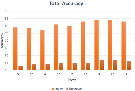
Figure 7.
Accuracy variation with layer configuration.
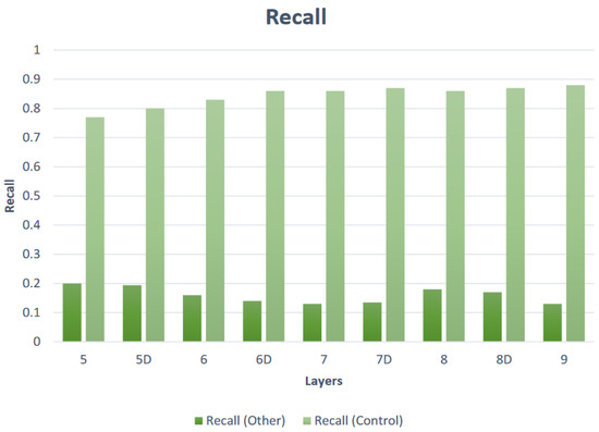
Figure 8.
Recall variation with layer configuration.
4.3. Optimized Model
The most promising model across all dataset experiments was the seven-layer dropout configuration, without other normalization techniques, training epochs below 10, and using ReLU activation function and an RMSProp optimizer. With these parameters, the model was able to not only correctly classify control data but also returned a clear and consistent confidence delta between control and unknown classes, firmly demonstrating that it can identify what it does not know. Figure 9 and Figure 10 show the class probabilities for control (green) and unknown (red) classes, the first for CIFAR-10 and K-49 experiments, respectively.
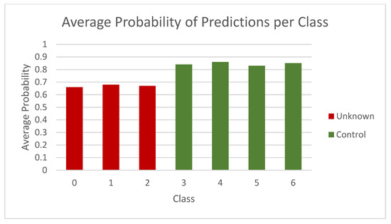
Figure 9.
Average probabilities for known (green) and unknown (red) classes, for CIFAR-10 experiment.
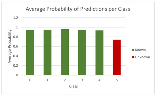
Figure 10.
Average probabilities for known and unknown classes for K-49.
The green bars show a high and uniform result, while the red bars are consistently lower and of similar value to each other. This creates a stable and useful delta, clearly observable in the visuals. When given a completely unknown datapoint, the model will return a confidence output well below that of control classes, meaning that a cut-off point for this can be easily assigned. For example, for any confidence result under 70% for CIFAR-10 in Figure 9, the network could highlight the datapoint as anomalous, suspicious, or generally unclassifiable. For the K49-MNIST selection in Figure 10, the confidence level on the unknown data is higher, but so is that of the control images, being well over 90% across the board. The model can therefore correctly classify expected data and recognize potential anomalies.
The experiment was repeated for the other aforementioned datasets, both independently and mixed, with a variety of image types. A useful delta was achievable in all cases, along with a strong recall for the known images. Delving deeper into individual datapoints, the attempted predictions for specific images can be observed, just as they were during model tuning. In Figure 11, the model has been presented with an image of a ship, which it has never previously encountered. The epistemic uncertainties bars are tall, indicating the consideration given to each potential label due to the lack of specific knowledge in the network. The probabilities reached all remain under 0.6. The model is extremely unsure of the classification of this image and “does not know” what the data is. In this instance, the “correct” label at (5) is a false positive from relabelling and encoding. This indicates that the model is performing as desired, refusing to assign any label with significant enough confidence.
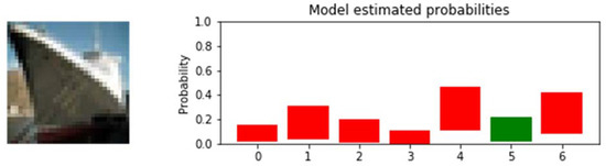
Figure 11.
Distributed label probabilities for unknown image (ship). Here, the green bar represents a false positive from relabelling, with the red bars indicating incorrect classification.
This is further seen in Figure 12, in which the model does not require much consideration to assign the correct label to a control test image of a frog. While other options are deliberated, this is brief, and the confidence in them is very low. The model selects the correct label (3) with high confidence, with the plot providing an insight into the inner workings of the classification process, i.e., contemplation against known possibilities.
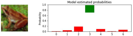
Figure 12.
Distributed label probabilities for control image (frog). The red and green bars represent incorrect and correct classifications respectively.
Another goal of this study was to maintain strong metrics across a variety of mixed sets and levels of openness. A range of levels was tested in experiments, and the results are presented in Figure 13 along with those from a study using Support Vector Machines in a probabilistic approach to OSR [23].
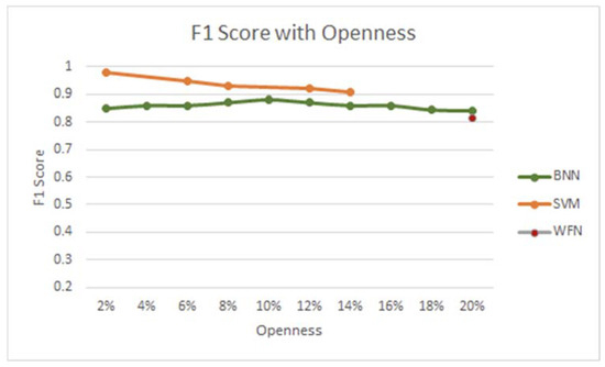
Figure 13.
F1 score change with dataset openness.
4.4. OSR Comparisons
As indicated in Table 1, the BNN method offers strong results alongside other approaches where the works are comparable, as well as offering insight into the model’s workings through distribution plotting and uncertainty analysis. This in turn leads to improved custom tuning, better generalization, and progress towards overcoming the openness problem experienced in other studies.

Table 1.
Comparison of older relevant studies to BNN results.
It is worth noting that the comparison study results focused only on a single grayscale dataset, rather than more complex custom ones, and the openness levels tested in this study went up to 14%. The scores for the BNN represent the averages for mixed colour and mixed grayscale sets. While the SVM results are higher for the levels tested, there is a noticeable descent compared to a steadier line formed by the BNN results. The openness levels seem to have less of an impact on the score for the Bayesian Neural Network approach; the SVM loses 0.8 from the score across a difference of 12%, compared to a 0.4 drop for the BNN across 18%. Specifics of the WildFishNet openness levels could not be determined outside of the 20% experiment, so this is featured alone in red, with the BNN result presenting a slightly higher score. This approach can therefore demonstrably compete with other methods in this regard.
The ODR accuracy of the BNN method is shown alongside recent novel approaches in Figure 14. There is a mix of data types: sound waves for GRU-CAE [25], colour images for WildFishNet [27], and generated nuclear industrial data for SVM-PMD [26]. All reach promising levels of accuracy, and the BNN results demonstrate that the methods proposed here can compete with other emerging ideas and experiments.
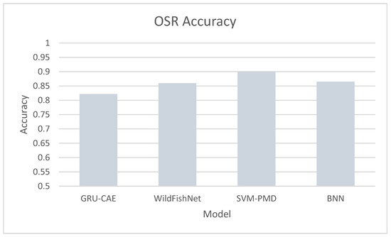
Figure 14.
Accuracy of different OSR techniques.
5. Conclusions and Further Work
This research has demonstrated that the proposed Bayesian Neural Network technique can be effective when used to build an agnostophilic AI system that recognizes the limits of its knowledge, returning unseen and unknown data that it finds unclassifiable based on probability distributions. Strong accuracy and reliability metrics are maintained, and the method works on a variety of image data. Further work would expand on the image data used as well as venturing into other data types for more impactful use cases. More investigation into openness levels would also be an area of exploration, as experiments so far suggest that the model reacts differently to this factor than do other approaches.
Author Contributions
S.M. performed the research and wrote the main paper. S.R. provided technical review and direction, and recommendations on language clarity and structure. V.R. provided technical review and recommendations for visuals. All authors have read and agreed to the published version of the manuscript.
Funding
This research received no external funding.
Institutional Review Board Statement
Not applicable to this study.
Data Availability Statement
All datasets used can be found in the References section. The Python code used for data preparation and experiments can be found at https://github.com/McBudner25/BNN_OSR/ (accessed on 31 March 2025).
Conflicts of Interest
The authors have no competing interests to declare that are relevant to the content of this article.
References
- Geng, C.; Huang, S.; Chen, S. Recent Advances in Open Set Recognition: A Survey. IEEE Trans. Pattern Anal. Mach. Intell. 2021, 43, 3614–3631. [Google Scholar] [CrossRef] [PubMed]
- MSalehi, M.; Mirzaei, H.; Hendrycks, D.; Li, Y.; Rohban, M.H.; Sabokrou, M. A Unified Survey on Anomaly, Novelty, Open-Set, and Out-of-Distribution Detection: Solutions and Future Challenges. arXiv 2021, arXiv:2110.14051. [Google Scholar]
- Pang, G.; Shen, C.; Hengel, A.; Cao, L. Toward Deep Supervised Anomaly Detection: Reinforcement Learning from Partially Labeled Anomaly Data. In Proceedings of the 27th ACM SIGKDD Conference on Knowledge Discovery and Data Mining, Singapore, 14–18 August 2021. [Google Scholar]
- Alloqmani, A.; Abushark, Y.; Khan, A.; Alsolami, F. Deep Learning based Anomaly Detection in Images: Insights, Challenges and Recommendations. Int. J. Adv. Comput. Sci. Appl. 2021, 12, 205–216. [Google Scholar] [CrossRef]
- Chopra, P. Bayesian NNs Using Pyro and PyTorch. TDS, 27 November 2018. Available online: https://medium.com/data-science/making-your-neural-network-say-i-dont-know-bayesian-nns-using-pyro-and-pytorch-b1c24e6ab8cd (accessed on 1 April 2025).
- Fan, W.; Miller, M.; Stolfo, S.; Lee, W.; Chan, P. Using Artificial Anomalies to Detect Unknown and Known Network Intrusions. In Proceedings of the 2001 IEEE International Conference on Data Mining, San Jose, CA, USA, 29 November–1 December 2001. [Google Scholar]
- Li, X.; Fei, J.; Xie, J.; Li, D.; Jiang, H.; Wang, R.; Qi, Z. Open Set Recognition for Malware Traffic via Predictive Uncertainty. Electronics 2023, 12, 323. [Google Scholar] [CrossRef]
- Nguyen, A.; Yosinski, J.; Clune, J. Deep neural networks are easily fooled: High confidence predictions for unrecognizable images. In Proceedings of the IEEE Conference on Computer Vision and Pattern Recognition, Boston, MA, USA, 7–12 June 2015; pp. 427–436. [Google Scholar]
- Chollet, F. Deep Learning with Python; Manning Publications: Shelter Island, NY, USA, 2018. [Google Scholar]
- Rosebrock, A. Anomaly Detection with Keras, TensorFlow, and Deep Learning. Pyimagesearch. 2 March 2020. Available online: https://pyimagesearch.com/2020/03/02/anomaly-detection-with-keras-tensorflow-and-deep-learning/ (accessed on 12 September 2024).
- Sermanet, P.; Eigen, D.; Zhang, X.; Mathieu, M.; Fergus, R.; LeCun, Y. OverFeat: Integrated Recognition, Localization and Detection using Convolutional Networks. In Proceedings of the 2nd International Conference on Learning Representations, Banff, AB, Canada, 12–14 April 2014. [Google Scholar]
- Chow, C. On optimum recognition error and reject tradeoff. IEEE Trans. Inf. Theory 1970, 16, 41–46. [Google Scholar] [CrossRef]
- Grandvalet, Y.; Rakotomamonjy, A.; Keshet, J.; Canu, S. Support vector machines with a reject option. In Advances in Neural Information Processing Systems; Morgan Kaufmann Publishers Inc.: San Francisco, CA, USA, 2009; pp. 537–544. [Google Scholar]
- Geifman, Y.; Ran, E.Y. Selective classification for deep neural networks. In Advances in Neural Information Processing Systems; Morgan Kaufmann Publishers Inc.: San Francisco, CA, USA, 2017; pp. 4872–4887. [Google Scholar]
- TensorFlow. mnist_corrupted. TensorFlow, 2022 (Updated). Available online: https://www.tensorflow.org/datasets/catalog/mnist_corrupted (accessed on 10 September 2024).
- Varga, D. Understanding How Image Quality Affects Transformer Neural Networks. Signals 2024, 5, 562–579. [Google Scholar] [CrossRef]
- Kang, C. Bayesian Convolutional Neural Network. Github, 26 August 2021. Available online: https://goodboychan.github.io/python/coursera/tensorflow_probability/icl/2021/08/26/01-Bayesian-Convolutional-Neural-Network.html (accessed on 10 September 2024).
- Cardoso, D.O.; Gama, J.; França, F.M.G. Weightless neural networks for open set recognition. Mach. Learn. 2017, 106, 1547–1567. [Google Scholar] [CrossRef]
- Bendale, A.; Boult, T.E. Towards open set deep networks. In Proceedings of the IEEE Conference on Computer Vision and Pattern Recognition, Las Vegas, NV, USA, 27–30 June 2016; pp. 1563–1572. [Google Scholar]
- Kardan, N.; Stanley, K. Fitted Learning: Models with Awareness of Their Limits; Department of Computer Science, University of Central Florida: Orlando, FL, USA, 2016. [Google Scholar]
- Zhang, W.; Huang, D.; Zhou, M.; Lin, J.; Wang, X. Open-Set Signal Recognition Based on Transformer and Wasserstein Distance. Appl. Sci. 2023, 13, 2151. [Google Scholar] [CrossRef]
- Xue, H.; Qin, J.; Quan, C.; Ren, W.; Gao, T.; Zhao, J. Open Set Sheep Face Recognition Based on Euclidean Space Metric. Math. Probl. Eng. 2021, 2021, 3375394. [Google Scholar] [CrossRef]
- Dhamija, A.R.; Gunther, M.; Boult, T. Reducing Network Agnostophobia. In Proceedings of the 32nd Conference on Neural Information Processing Systems, Montreal, QC, Canada, 2–8 December 2018. [Google Scholar]
- Scheirer, W.J.; Jain, L.P.; Boult, T.E. Probability Models for Open Set Recognition. IEEE Trans. Pattern Anal. Mach. Intell. 2014, 36, 2317–2324. [Google Scholar] [CrossRef] [PubMed]
- Yang, H.; Zheng, K.; Li, J. Open set recognition of underwater acoustic targets based on GRU-CAE collaborative deep learning network. Appl. Acoust. 2022, 193, 108774. [Google Scholar] [CrossRef]
- LLi, J.; Lin, M.; Wang, B.; Tian, R.; Tan, S.; Li, Y.; Chen, J. Open set recognition fault diagnosis framework based on convolutional prototype learning network for nuclear power plants. Energy 2024, 290, 130101. [Google Scholar] [CrossRef]
- Zhang, X.; Huang, B.; Chen, G.; Radenkovic, M.; Hou, G. WildFishNet: Open Set Wild Fish Recognition Deep Neural Network with Fusion Activation Pattern. IEEE J. Sel. Top. Appl. Earth Obs. Remote Sens. 2023, 16, 7303–7314. [Google Scholar] [CrossRef]
- Pavez, J.; Allende, H. A Hybrid System Based on Bayesian Networks and Deep Learning for Explainable Mental Health Diagnosis. Appl. Sci. 2024, 14, 8283. [Google Scholar] [CrossRef]
- Graves, A. Practical Variational Inference for Neural Networks. In Proceedings of the Conference on Neural Information Processing Systems, Granada, Spain, 12–15 December 2011. [Google Scholar]
- Varian, H.R. Big Data: New Tricks for Econometrics. J. Econ. Perspect. 2017, 28, 3–28. [Google Scholar] [CrossRef]
- Hüllermeier, E.; Waegeman, W. Aleatoric and epistemic uncertainty in machine learning: An introduction to concepts and methods. Mach. Learn. 2021, 110, 457–506. [Google Scholar] [CrossRef]
Disclaimer/Publisher’s Note: The statements, opinions and data contained in all publications are solely those of the individual author(s) and contributor(s) and not of MDPI and/or the editor(s). MDPI and/or the editor(s) disclaim responsibility for any injury to people or property resulting from any ideas, methods, instructions or products referred to in the content. |
© 2025 by the authors. Licensee MDPI, Basel, Switzerland. This article is an open access article distributed under the terms and conditions of the Creative Commons Attribution (CC BY) license (https://creativecommons.org/licenses/by/4.0/).