Uncertainty-Aware δ-GLMB Filtering for Multi-Target Tracking

Abstract

The $\delta$-GLMB filter is an analytic solution to the multi-target Bayes recursion used in multi-target tracking. It extends the Generalised Labelled Multi-Bernoulli (GLMB) framework by providing an efficient and scalable implementation while preserving track identities, making it a widely used approach in the field. Theoretically, the $\delta$-GLMB filter handles uncertainties in measurements in its filtering procedure. However, in practice, degeneration of the measurement quality affects the performance of this filter. In this paper, we discuss the effects of increasing measurement uncertainty on the $\delta$-GLMB filter and also propose two heuristic methods to improve the performance of the filter in such conditions. The base idea of the proposed methods is to utilise the information stored in the history of the filtering procedure, which can be used to decrease the measurement uncertainty effects on the filter. Since GLMB filters have shown good results in the field of multi-target tracking, an uncertainty-immune $\delta$-GLMB can serve as a strong tool in this area. In this study, the results indicate that the proposed heuristic ideas can improve the performance of filtering in the presence of uncertain observations. Experimental evaluations demonstrate that the proposed methods enhance track continuity and robustness, particularly in scenarios with low detection rates and high clutter, while maintaining computational feasibility.

1. Introduction

Multi-target tracking (MTT) is the procedure of estimating a time-varying number of targets and their states from a sequence of observations. The number of targets is usually unknown, and the observations are noisy due to the uncertainty of detection and presence of spurious targets (clutter) [1,2,3,4,5]. The trajectory of a target is another important outcome of MTT. Ref. [6] proposes a Bayesian multi-target tracking solution that also provides estimates of target trajectories. MTT suffers from the main challenges of detection uncertainty and clutter, which mislead the tracker and cause efficiency reduction in estimating the number of targets, their states, and their trajectories. However there are many approaches to MTT, and three paradigms are discussed as the main solutions. These are Multiple Hypotheses Tracking (MHT) [7,8,9], Joint Probabilistic Data Association (JPDA) [10,11,12], and Random Finite Set (RFS) [13,14,15,16]. Using the RFS approach in MTT provides a sophisticated Bayesian formulation for this problem in which a group of target states (multi-target states) are considered as a finite set [17,18]. This framework is a very popular method for estimating multi-targets, with applications in computer vision [19,20], robotics [21,22,23], sonar [24,25,26], monitoring and surveillance systems [27,28], sensor networks [29,30,31], cell biology [32,33], augmented reality [34,35], etc. In the RFS approach, the density of multi-target states is propagated recursively forward in time using the Bayes multi-target filter [36]. The Bayes filter is a multi-target tracker in which target specifications are incorporated into individual states (whereas in the RFS method, states of multi-targets in a unit of time are incorporated in a single set). Since the Bayes multi-target filter is intractable due to intense numerical complexity, the Probability Hypothesis Density (PHD) [37], Cardinalised PHD (CPHD) [38], and Multi-Bernoulli filters [39] were developed as approximations to the Bayes filter. In this work, we concentrate on an analytic solution to the Bayes MTT known as the $\delta$-Generalised Labelled Multi-Bernoulli ($\delta$-GLMB) framework, which uses the RFS notion of perceiving targets as distinguishable and unique entities. This filter is applicable to keeping trajectories, and it includes conjugate priors, which are closed under the Chapman–Kolmogrov equation. However, while results in [40,41,42] show promising performances of this filter, the performance of the filter decreases in situations where observation quality drops. The aim of this paper is to reduce the effect of a low detection rate and the existence of clutter on the $\delta$-GLMB filtering procedure. Consequent to the mentioned weakness, in particular, we propose two methods, N-scan $\delta$-GLMB and refined $\delta$-GLMB, to alleviate uncertainties in the observations using the information that is extracted from the history of filtering during a set time, which we believe to contain useful information that can be used to decrease uncertainties. The key innovation is to detect the components which are considered for truncation in the filtering procedure bur whose truncation may cause targets to get lost due to a low detection rate. Detecting such situations is verified from the aspect of considering the filtering history during the running time. The keyword N-scan is adopted from [43], and it is utilised in order to refer to the concept of using the history of information in a certain window with size N.

This paper is organised as follows. A brief overview of RFS, Bayesian multi-target filtering, and the GLMB filter is provided in Section 2. In Section 3, N-scan $\delta$-GLMB and refined $\delta$-GLMB are introduced and discussed. Results of numerical examples are discussed in Section 4, and concluding remarks and extensions are discussed in Section 5.

2. Background

This section gives a summary of the labelled RFS formulation of the MTT and the $\delta$-GLMB filter proposed in [41], along with implementation details from [40]. For clarity,

Table 1. Summary of notation.

Notation	Description
x	Single-target state
X	Multi-target state (set of targets)
$\mathbb{X}$	State space
Z	Multi-object measurement set
$\mathbb{L}$	Label space
ℓ	Unique label assigned to a target
${\delta }_Y\left(X\right)$	Generalised Kronecker delta function
$1_Y\left(X\right)$	Indicator function
$P_D(x,\ell )$	Probability of detection for target $(x,\ell )$
$g\left(z\right|x,\ell )$	Likelihood of measurement z given target $(x,\ell )$
$\pi \left(X\right)$	Multi-target probability density
$\Delta \left(X\right)$	Distinct label indicator function
$w^{(I,\xi )}$	Hypothesis weight
$p^{\left(\xi \right)}$	Probability density of target state

provides a summary of the notation used throughout this paper.

The standard inner product notation is shown as $\langle f,g\rangle \triangleq \int f\left(x\right)g\left(x\right)dx$. For a real valued function h, the notation of the multi-object exponential is shown as $h^X\triangleq {\Pi }_{x\in X}h\left(x\right)$, where $h^{\varnothing }=1$ by convention. For a given set X, the cardinality (element count) is denoted by $\left|X\right|$. The generalisation ${\delta }_Y\left(X\right)$ of the Kroneker delta allows the input argument to be in any arbitrary form, such as vectors, sets, etc. Similarly, the indicator function $1_Y\left(X\right)$ can be generalised such that it returns a value of 1 when $X\subseteq Y$.

2.1. Labelled Random Finite Sets (RFS)

The RFS is a random variable finite set which includes a random number of unordered points [14]. Since the number of points is random, it is possible to consider a cardinality distribution for the RFS. The collection of target states is treated as an RFS with a certain cardinality distribution which enables MTT without knowing the number of targets in the system. Labelled RFS is an extension of RFS, keeping track of each target identity. For this purpose, each target state $x\in \mathbb{X}$ is augmented with a unique unobserved label drawn from a discrete countable space $\ell \in \mathbb{L}=\{{\alpha }_i:i\in \mathbb{N}\}$, where the ${\alpha }_i$s are distinct and $\mathbb{N}$ denotes a positive integer set.

2.1.1. Bernoulli RFS

The probability density of a Bernoulli RFS X on $\mathbb{X}$ is denoted by [44]

$$\pi \left(X\right)=\left\{\begin{array}{cc}1-r,\hfill & X=\varnothing \hfill \\ r·p\left(x\right),\hfill & X=\left\{x\right\}.\hfill \end{array}\right.$$

(1)

where r is the probability that the RFS has only one element and $1-r$  is the probability that the RFS is empty. The elements inside the RFS (in the case of existence) are distributed according to the probability density $p(·)$. The Bernoulli RFS cardinality is itself Bernoulli distributed with parameter r.

2.1.2. Multi-Bernoulli RFS

A Multi-Bernoulli RFS X consists of the union of multiple independent Bernoulli RFS $X^{\left(i\right)}$ with existence probability $r^{\left(i\right)}\in (0,1)$ for $i=1,\cdots ,M$, i.e., $X={\cup }_{i=1}^M{X}^{\left(i\right)}·p(·)$. In [41], a Multi-Bernoulli RFS is described by $\pi ={\left\{(r^{\left(i\right)},p^{\left(i\right)})\right\}}_{i=1}^M$.

2.1.3. Labelled Multi-Bernoulli RFS

In [41], there is a derivation which shows that the following formulation is an alternative form of the LMB mentioned in Appendix A:

$$\pi \left(X\right)=\Delta \left(X\right)1_{\alpha (\Psi )}\left(\mathcal{L}\left(X\right)\right){[\Phi (X;·)]}^{\Psi }$$

(2)

where $\Delta \left(X\right)$ denotes the distinct label indicator ${\delta }_{\left|X\right|}\left(\right|\mathcal{L}\left(X\right)\left|\right)$ and $\mathcal{L}$ is a function defined on $\mathcal{L}:\mathbb{X}\times \mathbb{L}\to \mathbb{L}$ and a projection $\mathcal{L}\left(\right(x,\ell \left)\right)=\ell$; hence, $\mathcal{L}\left(X\right)=\left\{\mathcal{L}\right(x):x\in X\}$ is the X labels set. The parameter $\Phi (X;·)$ is defined as [41]

$${\displaystyle \Phi (X;\zeta )=\sum _{(x,\ell )\in X}{\delta }_{\alpha \left(\zeta \right)}(\ell )r^{\left(\zeta \right)}{p}^{\left(\zeta \right)}\left(x\right)+(1-1_{\mathcal{L}\left(X\right)}\left(\alpha \left(\zeta \right)\right))\left(1-r^{\left(\zeta \right)}\right)}$$

(3)

It is remarkable that a labelled RFS and its unlabelled version have the same cardinality distribution (proposition 2 in [41]).

2.2. Generalised Labelled Multi-Bernoulli RFS

The Generalised Labelled Multi-Bernoulli (GLMB) RFS is a family of labelled RFS distributions. GLMB is closed under the multi-object Chapman–Kolmogorov equation with respect to the multi-object transition kernel [41]. The probability density of a GLMB RFS X on $\mathbb{X}$ is denoted by

$${\displaystyle \pi \left(X\right)=\Delta \left(X\right)\sum _{\xi \in \Xi }{w}^{\left(\xi \right)}\left(\mathcal{L}\left(X\right)\right){\left[p^{\left(\xi \right)}\right]}^X}$$

(4)

where $\Xi$ is a discrete index set. The non-negative weight term $w^{\left(\xi \right)}\left(L\right)$ and the exponential term $p^{\left(\xi \right)}$ satisfy

$${\displaystyle \sum _{L\in \mathbb{L}}\sum _{\xi \in \Xi }{w}^{\left(\xi \right)}\left(L\right)=1,\int p^{\left(\xi \right)}(x,\ell )dx=1.}$$

(5)

A GLMB family can be understood as a mixture of multi-target exponentials for which its points are not statistically independent.

2.3. Bayesian Multi-Target Filtering

MTT is used to jointly estimate the number of targets and their states from measured observations. Due to the dynamic nature of the MTT problem, the number of targets changes over time. In MTT, the targets $X_k=\{x_{k,1},\cdots ,x_{k,N\left(k\right)}\}$ and observations $Z_k=\{z_{k,1},\cdots ,z_{k,M\left(k\right)}\}$ are considered as random finite sets, where k is the indicator of time, $N\left(k\right)$ is the number of targets, and $M\left(k\right)$ is the number of observations. Some observations may be clutter and others may be missed according to an underlying probability density. $g_k(·|·)$ is the multi-target likelihood function at time k which encapsulates the underlying models for clutter and detection. $f_{k|k-1}(·|·)$ is the multi-target transition density at time k which encapsulates the underlying models of births, spawns, deaths, and target motions. The multi-target Bayes filter propagates ${\pi }_k$ in time [44] according to the following update and prediction steps:

$${\pi }_k\left(X_k\right|Z_k)={\displaystyle \frac{g_k\left(Z_k\right|X_k){\pi }_{k|k-1}\left(X_k\right)}{\int g_k\left(Z_k\right|X){\pi }_{k|k-1}\left(X\right)\delta X}},$$

(6)

$${\pi }_{k+1|k}\left(X_{k+1}\right)=\int f_{k+1|k}\left(X_{k+1}\right|X_k){\pi }_k\left(X_k\right|Z_k)\delta X_k$$

(7)

2.4. Measurement Likelihood Function

The multi-object observation set $Z=\{z_1,\cdots ,z_{\left|Z\right|}\}$ is a union of detected states and clutter. Each state $(x,\ell )\in X$ is either detected with probability $P_D(x,\ell )$ or missed with $1-P_D(x,\ell )$. If the state is detected, it generates an observation point z with likelihood $g\left(z\right|x,\ell )$. Considering independent detection conditioned on X and independent clutter with a Poisson distribution with intensity $\kappa$, the multi-object likelihood function is denoted by

$${\displaystyle g\left(Z\right|X)=e^{-\langle \kappa ,1\rangle }{\kappa }^Z\sum _{\theta \in \Theta \left(\mathcal{L}\right(X\left)\right)}{\left[{\psi }_Z(·;\theta )\right]}^X}$$

(8)

where

$${\psi }_Z(x,\ell ;\theta )=\left\{\begin{array}{cc}{\displaystyle \frac{p_D(x,\ell )g\left(z_{{\theta }_{(\ell )}}\right|x,\ell )}{\kappa \left(z_{{\theta }_{(\ell )}}\right)}},\hfill & \mathrm{if}{\theta }_{(\ell )}>0\hfill \\ 1-p_D(x,\ell ),\hfill & \mathrm{if}{\theta }_{(\ell )}=0\hfill \end{array}\right.$$

(9)

2.5. Delta-Generalised Labelled Multi-Bernoulli

Delta-Generalised Labelled Multi-Bernoulli ($\delta$-GLMB) is an analytic solution to Bayes multi-target filtering. The numerical implementation of GLMB is ambiguous, so in order to address the ambiguity, $\delta$-GLMB offers an alternative form,

$${\displaystyle \pi \left(X\right)=\Delta \left(X\right)\sum _{(I,\xi )\in \mathcal{F}\left(\mathbb{L}\right)\times \Xi }{w}^{(I,\xi )}{\delta }_I\left(\mathcal{L}\left(X\right)\right){\left[p^{\left(\xi \right)}\right]}^X}$$

(10)

Substituting $w^{\left(\xi \right)}\left(I\right)$ with $w^{(I,\xi )}$ in Equation (4) simplifies the numerical implementation [40].

The $\delta$-GLMB filter, particularly the prediction step, is conditioned on measurements observed up to time k. The discrete space $\Xi$ contains the association map histories from the initial point of filtering history up to the present time of filtering [40]. ${\Theta }_t$ shows the association map space at time t; thus, $\Xi$ can be defined as ${\Theta }_{0:k}\triangleq {\Theta }_0\times \cdots \times {\Theta }_k$. Hence, the update and prediction densities of $\delta$-GLMB are denoted as

$${\displaystyle {\pi }_k\left(X\right|Z_k)=\Delta \left(X\right)\sum _{(I,\xi )\in \mathcal{F}\left({\mathbb{L}}_{0:k}\right)\times {\Theta }_{0:k}}{w}_k^{(I,\xi )}{\delta }_I\left(\mathcal{L}\left(X\right)\right){\left[p_k^{\left(\xi \right)}(·|Z_k)\right]}^X}$$

(11)

$${\displaystyle {\pi }_{k+1|k}\left(X\right)=\Delta \left(X\right)\sum _{(I,\xi )\in \mathcal{F}\left({\mathbb{L}}_{0:k+1}\right)\times {\Theta }_{0:k}}{w}_{k+1|k}^{(I,\xi )}{\delta }_I\left(\mathcal{L}\left(X\right)\right){\left[p_{k+1|k}^{\left(\xi \right)}\right]}^X}$$

(12)

where $\xi =({\theta }_0,\cdots ,{\theta }_k)$, ${\theta }_k\in {\Theta }_{0:k}$ is an association history map up to time k. Considering $I\in \mathcal{F}\left({\mathbb{L}}_{0:k}\right)$ as a representation of a track label at time k, the pair $(I,\xi )\in \mathcal{F}\left({\mathbb{L}}_{0:k}\right)\times {\Theta }_{0:k}$ is known as a hypothesis with weight $w_k^{(I,\xi )}$. $p^{\left(\xi \right)}$ is the density of the kinematic state of track ℓ for each $\xi$. Bayesian recursion is used to propagate the densities forward in time in a closed-form update step [40]:

$${\displaystyle \pi \left(X\right|Z)=\Delta \left(X\right)\sum _{(I,\xi )\in \mathcal{F}\left(\mathbb{L}\right)\times \Xi }\sum _{\theta \in \Theta \left(I\right)}{w}^{(I,\xi ,\theta )}\left(Z\right){\delta }_I\left(\mathcal{L}\left(X\right)\right){\left[p^{(\xi ,\theta )}(·|Z)\right]}^X}$$

(13)

where $\Theta \left(I\right)$ denotes association maps which are related to components with identity domain I,

$$w^{(I,\xi ,\theta )}\left(Z\right)\propto w^{(I,\xi )}{\left[{\eta }_Z^{(\xi ,\theta )}\right]}^I,$$

(14)

$${\eta }_Z^{(\xi ,\theta )}(\ell )=\langle p^{\xi }(·,\ell ),{\psi }_Z(·,\ell ;\theta )\rangle ,$$

(15)

$$p^{(\xi ,\theta )}(x,\ell |Z)={\displaystyle \frac{p^{\left(\xi \right)}(x,\ell )\psi (x,\ell ;\theta )}{{\eta }_Z^{(\xi ,\theta )}(\ell )}},$$

(16)

The prediction step is given by

$${\displaystyle {\pi }_{+}\left(X_{+}\right)=\Delta \left(X_{+}\right)\sum _{(I_{+},\xi )\in \mathcal{F}\left({\mathbb{L}}_{+}\right)\times \Xi }{w}_{+}^{(I_{+},\xi )}{\delta }_{I_{+}}\left(\mathcal{L}\left(X_{+}\right)\right){\left[p_{+}^{\left(\xi \right)}\right]}^{X_{+}}}$$

(17)

Considering S as a survival component indicator, B as newly born ones, ⊇ for the super set, and the subscript + for time $k+1$:

$$w_{+}^{(I_{+},\xi )}=w_S^{\left(\xi \right)}(I_{+}\cap \mathbb{L})w_B(I_{+}\cap \mathbb{B})$$

$${\displaystyle w_S^{\left(\xi \right)}\left(L\right)={\left[{\eta }_S^{\left(\xi \right)}\right]}^L\sum _{I\supseteq L}{[1-{\eta }_S^{\left(\xi \right)}]}^{I-L_{w^{(I,\xi )}}}}$$

$${\eta }_S^{\left(\xi \right)}(\ell )=\langle p_S(·,\ell ),p^{\left(\xi \right)})(·,\ell )\rangle$$

(18)

$$p_{+}^{\left(\xi \right)}(x,\ell )=1_{\mathbb{L}}(\ell )p_S^{\left(\xi \right)}(x,\ell )+1_{\mathbb{B}}(\ell )p_B(x,\ell )$$

$$p_S^{\left(\xi \right)}(x,\ell )={\displaystyle \frac{\langle p_S(·,\ell )f\left(x\right|·,\ell ),p^{\left(\xi \right)}(·,\ell )\rangle }{{\eta }_S^{\left(\xi \right)}(\ell )}}$$

2.6. N-Scan GM-PHD Filter

The GM-PHD filter was proposed [45] as a closed-form solution to the PHD filter [37]. The GM-PHD filter models each target with a Gaussian component with an associated weight ($w_K^i$), mean ($m_k^i$), and covariance ($S_k^i$). After performing the prediction and update, this filter extracts the Gaussian components whose weights are greater than a predefined threshold to estimate the multi-target states at each step and discards those components as non-informative [45]. This pruning is not always effective: if the measurement of the target is uncertain, the weight of the target is significantly decreased and the estimation of the target is lost. Ref. [43] proposes an N-scan approach which improves performance by benefiting from the last N target steps to avoid missing the estimation of the targets having different uncertainties. N-scan GM-PHD defines each Gaussian component with extra parameters to improve tracking performance: a binary confidence ${\theta }^i$, and weight history $W{H}^i$, containing the last N weights of $W{H}_k^i=[w_{k-N+1}^i,\cdots ,w_{k-1}^i,w_k^i]$. N-scan GM-PHD propagates parameter set $x_k^i=\langle w_K^i,m_k^i,S_k^i,{\theta }_k^i,W{H}_k^i\rangle$ in time, calculating the number of weights $W{H}_k^i$ which exceed a predefined threshold, and treats them with a new pruning policy which considers the whole N history window of weights [43].

3. Proposed Methods

Each iteration of the $\delta$-GLMB filter involves a prediction operation followed by an update operation. These operations generate multi-target exponential weighted sums [40], the number of terms of which are intractable due to super-exponential growth of the terms in time. It is not rational to exhaustively consider all the terms in computations; hence, it is obligatory to prune some terms. Multi-object densities are truncated by keeping the most informative terms with respect to their weights and discarding those deemed non-informative with respect to their insignificant weights (the components with a weight lower than a predefined threshold are truncated). This section analyses truncation in uncertain conditions and shows that the pruning phase of $\delta$-GLMB causes some terms to be truncated from the filtering procedure which are informative during a time window but whose weights have decreased at the moment due to uncertainty conditions like miss detection.

As a sequel to [46], which proposed the concept of N-scan $\delta$-GLMB, this section details the N-scan $\delta$-GLMB implementation and presents an enhanced update and prediction phase regarding the N-scan concept.

3.1. Uncertainty Effects on $\delta$-GLMB

In the $\delta$-GLMB filtering procedure, the pruning phase might cause weak performance in scenarios with a high uncertainty level (e.g., low detection probability, high clutter ratio, etc.). Suppose that one or more targets are not detected due to miss detection of these targets. Their associated hypotheses weight ($w^{(I,\xi )}$) will diminish; hence, the associated hypotheses of true tracks are removed from the filtering procedure and cause the filtering performance drop. Furthermore, from a mathematical point of view, as it is obvious in Equation (9), the low detection rate causes the parameter $\psi$ to decrease, and as a result, the multi-state target density decreases. In such conditions, losing true tracks produces a less informative approximation of the posterior distribution in Equation (11), which is clearly obviously inferred from Equations (13)–(15).

3.2. N-Scan $\delta$-GLMB

In the $\delta$-GLMB filtering procedure, there is a pruning operation that discards the hypotheses $(I,\xi )$ whose weights are lower than an empirical predefined threshold $W_{Th}$.

$${\Omega }_k=\{\forall (I,\xi )\in \mathcal{F}\left({\mathbb{L}}_k\right)\times {\Theta }_k|w_k^{(I,\xi )}\ge W_{Th}\}$$

(19)

where ${\Omega }_k$ is defined as the pool containing all hypotheses after pruning. All the hypotheses which exist in this pool continue in the filtering procedure, and those which do not exist anymore are discarded. As mentioned before, this operation occurs in order to prevent the hypotheses numbers from increasing exponentially during the set time and eventually making the filtering procedure intractable. This pruning and its sequel state extraction are not always effective, as pointed out in Section 3.1. Whenever the weight of a hypothesis degenerates below the threshold $W_{Th}$, the hypothesis is discarded; however, the weight devaluation of a hypothesis may be a sequence of miss detection or another uncertainty.

In this paper, a simple and effective N-scan approach [43,46] is used for truncating the hypotheses instead of discarding those with weights lower than an empirical, predefined threshold $W_{Th}$. Using the N-scan approach improves the performance of the previous methods, especially in scenarios with a lower SNR ratio which are considered to be uncertain conditions. The suggested method benefits from the N last history of the weights of hypotheses when faced with possible uncertainties. A $\delta$-GLMB is completely characterised by the set of parameters $\{(w^{(I,\xi )},p^{\left(\xi \right)}):(I,\xi )\in \mathcal{F}\left(\mathbb{L}\right)\times \Xi \}$. This paper follows [40], which considers the parameter set of $\delta$-GLMB as an enumeration of all hypotheses together with their weights and track densities. This assumption aims at easing the implementation procedure. Considering the mentioned assumption, the $\delta$-GLMB parameter set is shown as ${\{I_k^{\left(h\right)},{\xi }_k^{\left(h\right)},w_k^{\left(h\right)},p_k^{\left(h\right)}\}}_{h=1}^H$, where $w^{\left(h\right)}\triangleq w^{(I^{\left(h\right)},{\xi }^{\left(h\right)})}$ and $p^{\left(h\right)}\triangleq p^{\left({\xi }^{\left(h\right)}\right)}$. With respect to this presentation of the parameter set, the N-scan method adds two additional parameters, ${\gamma }^{\left(h\right)}$ and $W{H}^{\left(h\right)}$; therefore, the new parameter set is shown as follows:

$${\{I_k^{\left(h\right)},{\xi }_k^{\left(h\right)},w_k^{\left(h\right)},p_k^{\left(h\right)},{\gamma }_k^{\left(h\right)},W{H}_k^{\left(h\right)}\}}_{h=1}^H$$

(20)

where ${\gamma }^{\left(h\right)}$ is the binary confidence indicator for all hypotheses in $\mathbb{H}$. It determines whether a hypothesis h was discarded in previous iterations or not. The value of $\gamma$ for each hypothesis is initialised to zero at initiation of the hypotheses; whenever a hypothesis satisfies the extraction conditions, the value of ${\gamma }^{\left(h\right)}$ is changed to one. $W{H}^{\left(h\right)}$ is the weight history of each hypothesis $h\in \mathbb{H}$, which keeps the last N weights of a hypothesis h, i.e.,

$$W{H}_k^{\left(h\right)}=[w_{k-N+1}^{\left(h\right)},\cdots ,w_{k-1}^{\left(h\right)},w_k^{\left(h\right)}]$$

(21)

This extended version of the parameter set is propagated during the filtering procedure. The additional parameters are utilised to improve the tracking performance of the $\delta$-GLMB filter in more uncertain conditions. The overall steps of the proposed N-scan $\delta$-GLMB algorithm are summarised as follows.

3.2.1. Initialisation

In the $\delta$-GLMB filter, each hypothesis is initialised by a proper setting. In addition to that setting with regard to the new parameter set, ${\gamma }_0^{\left(h\right)}$ and $W{H}_0^{\left(h\right)}$ need to be initialised too. Since the newly born hypothesis has not been extracted before, the initial value for ${\gamma }_0^{\left(h\right)}$ is zero. All first $N-1$ elements of $W{H}_0^{\left(h\right)}$ are set to zero (no history is available before initialisation) and the $N^{th}$ element is set to the ordinary initialisation value of a hypothesis

$${\gamma }_0^{\left(h\right)}=1,$$

(22)

$$W{H}_0^{\left(h\right)}=[0,0,0,\cdots ,0,0,w_0^{\left(h\right)}]$$

(23)

where $|W{H}_k^{\left(h\right)}|=N$.

Note that the initialisation of a hypothesis may occur in the middle of the filtering time due to newborn targets or spawned targets. In this situation, the initialisation of $\gamma$ and $WH$ is the same as mentioned above.

3.2.2. Prediction

In the prediction step of the $\delta$-GLMB filter, the filtering density ${\pi }_{+}\left(X_{+}\right)$ is estimated as explained in Section 2.5. However, the estimation of the filtering density ${\pi }_{+}\left(X_{+}\right)$ in the N-scan method is not altered, and the newly defined parameters which are used in further steps propagate during this time. The following propagation schema is appended to the prediction step of the $\delta$-GLMB filter:

$${\gamma }_{k|k-1}^{\left(h\right)}={\gamma }_{k-1}^{\left(h\right)},$$

(24)

$$W{H}_{k|k-1}^{\left(h\right)}=W{H}_{k-1}^{\left(h\right)}$$

(25)

3.2.3. Update

In the update step of the $\delta$-GLMB filter, the filtering density $\pi \left(X\right|Z)$ is estimated by Equation (11). In addition to the estimation of $\pi \left(X\right|Z)$, which is in the presence of the observing measurements, the weight history of a hypothesis is updated too. The weight history updating procedure is denoted by

$$W{H}_k^{\left(h\right)}=[W{H}_{k|k-1}^{\left(h\right)}\left[2\right],W{H}_{k|k-1}^{\left(h\right)}\left[3\right],\cdots ,W{H}_{k|k-1}^{\left(h\right)}\left[N\right],w_k^{\left(h\right)}]$$

(26)

where $WH\left[\zeta \right]$ stands for the ${\zeta }^{th}$ element of vector WH. Intuitively, the update procedure of WH is equal to removing the first element of the vector WH (the oldest weight of hypothesis h) and adding the current weight of the hypothesis h to the weight history. Note that the order in the weight history matters, as it is an indicator of how old a weight is.

3.2.4. Pruning and Extraction

In $\delta$-GLMB filtering recursion, there is a pruning phase that intends to avoid exponential growth of the system by discarding hypotheses with insignificant weights. This paper benefits from new defined parameters $WH$ and $\gamma$ to alter the procedure of pruning. The N-scan version of $\delta$-GLMB does not discard the hypotheses whose weights are lower than $W_{Th}$ at iteration k because the degeneration of the hypotheses’ weight could be the result of a miss detection or another uncertainty in the observation. Similar to the idea in [43], utilising new parameters which are added to the hypothesis parameter set, this paper proposes a new discarding method, the results of which show that it outperforms the previous methods. The N-scan method tends to extract the hypotheses which satisfy either one of the following conditions and prune others:

Condition 1: ${\gamma }_k^{\left(h\right)}=0$ (i.e., the hypothesis h has not been extracted yet) and $N_{Tr}\ge N_{Init}$.

Condition 2: ${\gamma }_k^{\left(h\right)}=1$ (i.e., the hypothesis h has been extracted already) and $N_{Tr}\ge N_{Surv}$, where $N_{Tr}$ shows the number of weights in $W{H}_k^{\left(h\right)}$ which exceed $W_{Th}$, $N_{Init}$ shows the predefined threshold for extraction of newly born hypotheses, and $N_{Surv}$ is the threshold for surviving hypotheses.

Note that if the first condition is satisfied, then the value of ${\gamma }_k^{\left(h\right)}$ changes to one because the hypothesis h is now extracted. Algorithm 1 summarises the N-scan method.

Algorithm 1: Summary of N-scan pruning algorithm.

Intuitively, this method is proposed in order to give a second chance to hypotheses that are candidates for being discarded. Depending on the value of N, this chance may increase relatively. The idea behind giving a second chance to a hypothesis is to prevent truncation of informative hypotheses which belong to the true target; however, at the moment k, their observation is uncertain (e.g., due to miss detection); hence, their weights have dropped. However, when using the N-scan method for truncation, the hypotheses add a slight burden on the filtering procedure, and it helps to reduce missing valuable information due to uncertainties. In the following, the effect of the N-scan on the filtering is pointed out in more detail.

Intuitively, N-scan method treats hypotheses with a weight lower than $W_{Th}$ in an optimistic way. It considers the reduction of their weight as a result of an uncertainty. In a window with size N which contains the weight history of the hypotheses, if the elements exceed $W_{Th}$ at least $\vartheta$ times, then the hypothesis is extracted. Hence, the distribution of extraction is formulated following a form which is similar to a binomial trial:

$${\displaystyle {\pi }_{extraction}(x,\ell )=\sum _{i=0}^{N-\vartheta }\left(\genfrac{}{}{0pt}{}{N}{\vartheta +i}\right)p_{\hslash }^{\vartheta +i}(x,\ell ){(1-p_{\hslash }(x,\ell ))}^{N-\vartheta -i}}$$

(27)

where $p_{\hslash }(x,\ell )$ is the probability that $w^{(x,\ell )}$ is greater than $W_{Th}$, and this probability relates directly with $p_D(x,\ell )$, i.e., $p_{\hslash }(x,\ell )\propto p_D(x,\ell )$ (generally relates with uncertainty amount), $\vartheta =N_{Surv}$ for surviving hypotheses, and $\vartheta =N_{Init}$ for newly born hypotheses.

However, with the reduction of $P_D$, the $p_{\hslash }$ falls too at step k, and the other terms which are saved inside $WH$ are able to increase ${\pi }_{extraction}$; hence, the miss detection, or generally any reason that makes $p_{\hslash }$ degenerate, can be ignored for a restricted time period (relative to the size of $WH$). According to ${\pi }_{extraction}$, increasing the value of N makes the filtering procedure more immune to uncertainty in exchange for keeping more hypotheses, which complicates the system computations.

From another point of view, N-scan provides a super set of hypotheses as $\mathbb{H}=\mathbb{T}\cup \mathbb{C}$, where $\mathbb{H}$ is the space of all hypotheses, $\mathbb{T}$ is the space of the truncated hypotheses without using the N-scan method, and $\mathbb{C}$ is the space of hypotheses that the N-scan method considers as candidates for uncertain hypotheses. It is obvious that the space $\mathbb{C}$ is a super set of the two spaces ${\mathbb{C}}^T$ and ${\mathbb{C}}^F$, where ${\mathbb{C}}^T$ is the space of those hypotheses which are truly under a uncertain condition and N-scan is able to detect them (e.g., uncertainty in the observations lasts at most N iterations); hence, their weights are degenerated and ${\mathbb{C}}^F$ is the space of those hypotheses for which the degeneration in weight is not because of uncertainty (e.g., targets are dead and removed from observation permanently) or because the N-scan method, due to the value of parameter N, is not able to detect them as a member of ${\mathbb{C}}^T$. With regard to the definitions above, the N-scan method keeps $|C_k|$ extra hypotheses in iteration k, discards $|C_{i-(N-\vartheta )}^F|$ hypotheses, and detects $|C_{i-N-\vartheta }^T|$ as uncertain hypotheses in previous iterations which are now certain. Hence, the extracted hypotheses are $T\cup C^T$. However, in scenarios with certain observations, the N-scan method performs exactly like the traditional discarding method and adds an irrational overhead to the filtering procedure. This method is useful in uncertain conditions despite the overhead to the filtering procedure. It is a trade-off between better accuracy for MTT and a slight computation overhead. The $L_1$-error distance of the N-scan and traditional methods of discarding is investigated in Appendix B.

In the $\delta$-GLMB filtering, computing all the hypotheses first and then discarding them is an computationally intense process. Ref. [40] introduces methods to truncate hypotheses without propagating them. Ref. [40] utilises ranked assignment and K-shortest path algorithms incorporated with update and prediction processes to reach this goal. The following sections propose an alternative implementation of the update and prediction phases based on these tricks with regard to the N-scan concept, which tries to keep the hypotheses that are chosen wrongly as candidates for truncation due to a high uncertainty ratio. These enhanced update and prediction phases alleviate the implementation computation complexity of the $\delta$-GLMB filter and yet try to stay immune to the uncertainties.

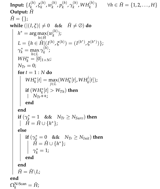
3.3. Enhanced Update Phase

Ref. [40] proposes a tractable implementation of the $\delta$-GLMB update which truncates the multi-target filtering density without computing all the hypotheses and their weights. This goal is achieved based on the idea which generates the association maps $\theta \in \Theta \left(I\right)$ in decreasing order of ${\left[{\eta }_Z^{(\xi ,\theta )}\right]}^I$ and selects the hypotheses with the highest weights. (As is clear in Equation (11), hypothesis $(I,\xi )$ generates a new set of hypotheses $(I,(\xi ,\theta ),\theta \in \Theta (I\left)\right)$ with weights $w^{(I,\xi ,\theta )}\left(Z\right)\propto w^{(I,\xi )}{\left[{\eta }_Z^{(\xi ,\theta )}\right]}^I$.) However, when using this idea, the highest weighted components are selected without computing all the possible hypotheses, and the chance of discarding hypotheses which have uncertainty in the current moment rises. In order to solve these problems simultaneously, the concept of scanning the history of the hypotheses’ condition in a certain N-sized windowing time is incorporated with the $\delta$-GLMB update method proposed in [40].

Let assignment matrix S be a representation for each association map $\theta \in \Theta \left(I\right)$ which has the dimension $\left|I\right|\times \left|Z\right|$ where $Z=\{z_1,\cdots ,z_{\left|Z\right|}\},$$I=\{{\ell }_1,\cdots ,{\ell }_{\left|I\right|}\}$. S consists of 0 or 1 entries where $S_{i,j}=1$ if and only if ${\theta }_{\left({\ell }_i\right)}=j$ (i.e., the jth measurement is assigned to track ${\ell }_i$), otherwise $S_{i,j}=0$. The optimal assignment cost matrix is denoted as a $\left|I\right|\times \left|Z\right|$ matrix [40]

$$C_Z^{(I,\xi )}=\left[\begin{array}{ccccc}{C}_{1,1}& C_{1,2}& C_{1,3}& \cdots & C_{1,\left|Z\right|}\\ C_{2,1}& C_{2,2}& C_{2,3}& \cdots & C_{2,\left|Z\right|}\\ ⋮& ⋮& ⋮& \ddots & ⋮\\ C_{\left|I\right|,1}& C_{\left|I\right|,2}& C_{\left|I\right|,3}& \cdots & C_{\left|I\right|,\left|Z\right|}\end{array}\right]$$

(28)

where

$$C_{i,j}=-ln\left({\displaystyle \frac{\langle p^{\left(\xi \right)}(·,{\ell }_i),p_D(·,{\ell }_i)g\left(z_j\right|·,{\ell }_i)\rangle }{\langle p^{\left(\xi \right)}(·,{\ell }_i),1-p_D(·,{\ell }_i)\rangle \kappa \left(z_j\right)}}\right)$$

(29)

when $i,j$ are both natural numbers, $1\le i\le \left|I\right|$ and $1\le j\le \left|Z\right|$.

The cost value above can be interpreted as the cost of assignment the jth measurement to track ${\ell }_i$. Then the cost of assignment of all the measurements to the tracks can be written as the Frobenius inner product of the cost matrix and assignment matrix

$${\displaystyle tr\left(S^T{C}_Z^{(I,\xi )}\right)=\sum _{i=1}^{\left|I\right|}\sum _{j=1}^{\left|Z\right|}{C}_{i,j}{S}_{i,j}}$$

(30)

In order to obtain an optimal assignment, an optimal assignment matrix ($S^{*}$) is needed which minimises the cost of $tr\left(S^{*T}{C}_Z^{(I,\xi )}\right)$. Note that each $S^{*}$ has a corresponding associate map ${\theta }^{*}$. For this purpose, the concept of the ranked assignment problem [47] is used. Such a problem tries to find an enumeration of the least cost assignment matrices in increasing order [48]. Hence, in the case of finding the optimal assignment for measurements to tracks in the $\delta$-GLMB filter for which the cost matrix is $C_Z^{(I,\xi )}$, the rank optimal assignment generates an enumeration of association maps $\theta$ in order of decreasing ${\left[{\eta }_Z^{(\xi ,\theta )}\right]}^I$. Since the optimal assignment is a combinatorial problem and also enumerates the least T cost assignment, the Murty [48] algorithm is used to solve this problem. Further details are available in [40].

Despite the effectiveness of the mentioned method for ease of implementation, the uncertainty of observations affects the cost value, which is the base of ranking algorithms used for truncation. As is obvious in Equation (34), the growth of uncertainty causes a $C_{i,j}$ increase. With the reduction of the detection rate, and consequently, a reduction in the measurement likelihood function $g\left(z_j\right|·,{\ell }_i)$ or/and in the growth of the clutter rate, the value inside the $-ln(·)$ drops, hence the cost value increase. Growth of the $C_{i,j}$ causes the corresponding hypothesis rank drops among the hypotheses ranks and consequently obtains a higher chance to be a candidate for truncation. This behaviour may cause an informative hypothesis to get truncated due to existence of the momentary uncertainties and the track of the object to get lost. From a different aspect, by substituting Equation (9) in Equation (15), another form of ${\left[{\eta }_Z^{(\xi ,\theta )}\right]}^I$ can be written as follows:

$${\displaystyle {\left[{\eta }_Z^{(\xi ,\theta )}\right]}^I=\exp \left(tr\left(S^T{C}_Z^{(I,\xi )}\right)\right)\prod _{\ell \in I}〈p^{\left(\xi \right)}(·,\ell ),1-p_{D(·,\ell )}〉}$$

(31)

which shows that the reduction of the cost matrix causes the value of ${\left[{\eta }_Z^{(\xi ,\theta )}\right]}^I$ to decrease, and consequently, the chance of discarding the corresponding hypothesis for track label I gets higher.

In order to increase the immunity of the update phase to uncertainties, we used the N-scan idea in the selection of the hypotheses according to the value of ${\left[{\eta }_Z^{(\xi ,\theta )}\right]}^I$ with slight differences, which is described in the following.

After sorting the association maps according to ${\left[{\eta }_Z^{(\xi ,\theta )}\right]}^I$ in decreasing order, the association maps with the highest value of ${\left[{\eta }_Z^{(\xi ,\theta )}\right]}^I$ (which is analogous to supposing that they are hypotheses that satisfy the condition ${\left[{\eta }_Z^{(\xi ,\theta )}\right]}^I\ge {\eta }^{Threshold}$) are considered as candidates for surviving. In contrast with the previously described update method, the rest of the association maps are not truncated.

Let M, T, and $T^{\prime }$ denote the set of all association maps, association maps which satisfy the condition ${\left[{\eta }_Z^{(\xi ,\theta )}\right]}^I\ge {\eta }^{Threshold}$, and the set of the rest of the association maps, respectively ($M=T\cup T^{\prime }$). The relevant hypotheses in the set T propagate into the next step (prediction step). Due to the uncertainty conditions, it is possible that the set $T^{\prime }$ contains association maps whose ${\left[{\eta }_Z^{(\xi ,\theta )}\right]}^I$ is decreased momentarily. The following schema is presented in order to find such association maps; however, their ${\left[{\eta }_Z^{(\xi ,\theta )}\right]}^I$ is under the ${\eta }^{Threshold}$. In the future of the filtering time, their ${\left[{\eta }_Z^{(\xi ,\theta )}\right]}^I$ will increase due to the annihilation of the uncertainties.

Considering a $\delta$-GLMB parameter set denoted by ${\{I_k^{\left(h\right)},{\xi }_k^{\left(h\right)},w_k^{\left(h\right)},p_k^{\left(h\right)}\}}_{h=1}^H$, the parameter ${\rm Y}$ is added in order to keep track of the value of

$${\displaystyle \frac{{\sum }_{j=1}^{T_k^{\left(h\right)}\cup T_k^{\prime \left(h\right)}}{\left[{\eta }_Z^{({\xi }_k^{\left(h\right)},{\theta }_k^{(h,j)})}\right]}^{I_k^{\left(h\right)}}}{|T_k^{\left(h\right)}\cup T_k^{\prime \left(h\right)}|}}$$

(32)

as an indicator for the amount of cumulative information stored in the hypotheses $(I,(\xi ,\theta \left)\right),\theta \in \Theta \left(I\right)$, which are generated by hypothesis $(I,\xi )$ during the filtering time. Therefore the parameter set is denoted by

$${\{I_k^{\left(h\right)},{\xi }_k^{\left(h\right)},w_k^{\left(h\right)},p_k^{\left(h\right)},{{\rm Y}}_k^{\left(h\right)}\}}_{h=1}^H$$

(33)

${{\rm Y}}^{\left(h\right)}$ is a history matrix which keeps the last N cumulative information stored in hypothesis $\left(h\right)$.

$${{\rm Y}}_k^{\left(h\right)}=[{\upsilon }_{k-N+1}^{\left(h\right)},\cdots ,{\upsilon }_{k-1}^{\left(h\right)},{\upsilon }_k^{\left(h\right)}]$$

(34)

where

$${\upsilon }_k^{\left(h\right)}={\displaystyle \frac{{\sum }_{j=1}^{T_k^{\left(h\right)}\cup T_k^{\prime \left(h\right)}}{\left[{\eta }_Z^{({\xi }_k^{\left(h\right)},{\theta }_k^{(h,j)})}\right]}^{I_k^{\left(h\right)}}}{|T_k^{\left(h\right)}\cup T_k^{\prime \left(h\right)}|}}.$$

(35)

In the rest of this section, according to the newly defined parameter ${\rm Y}$, a new truncation algorithm for the update phase of the $\delta$-GLMB filter is presented which is more immune to uncertain conditions.

The overall steps of the proposed truncation method are summarised as follows. The initialisation and ${\rm Y}$ propagation steps are almost the same as the N-scan method, with the history vector ${{\rm Y}}_0^{\left(h\right)}=[0,0,0,\cdots ,0,0,{\upsilon }_0^{\left(h\right)}]$, where $|{{\rm Y}}_k^{\left(h\right)}|=N$. An ordered enumeration of association maps $\theta$ is obtained after solving the ranked optimal assignment problem whose cost matrix is $C_Z^{(I,\xi )}$. This enumeration is sorted according to the value of ${\left[{\eta }_Z^{(\xi ,\theta )}\right]}^I$, which relates directly to the weight of a hypothesis $w^{(I,\xi ,\theta )}\left(Z\right)\propto w^{(I,\xi )}{\left[{\eta }_Z^{(\xi ,\theta )}\right]}^I$.

Analogous to [40], the hypotheses which satisfy the condition ${\left[{\eta }_Z^{(\xi ,\theta )}\right]}^I\ge {\eta }^{Threshold}$ (the set T) are chosen for being extracted in the next prediction step. Although the elements of the set T are selected, there might be hypotheses in the set $T^{\prime }$ whose value of ${\left[{\eta }_Z^{(\xi ,\theta )}\right]}^I$ is under a certain threshold; however, selecting them benefits the filtering procedure due to uncertainty reasons.

In the following, utilising the parameter ${\rm Y}$, a method is proposed for detecting some candidates $C\subseteq T^{\prime }$ which are probable victims of uncertainty reasons that cause the value ${\left[{\eta }_Z^{(\xi ,\theta )}\right]}^I$ of a hypothesis to decrease.

A hypothesis $\left(h\right)$ is added to the candidate set C if it satisfies either one of the following conditions:

Condition 1:

$${\displaystyle \sum _{i=0}^{|{{\rm Y}}_k^{\left(h\right)}|-1}\frac{{{\rm Y}}_k^{\left(h\right)}\left[i\right]}{|{{\rm Y}}_k^{\left(h\right)}|}\ge {\upsilon }_{Mean}}$$

(36)

and

$$\begin{array}{c}Var({{\rm Y}}_k^{\left(h\right)}[0:|{{\rm Y}}_k^{\left(h\right)}|-1])-\\ \\ Var({{\rm Y}}_k^{\left(h\right)}[0:|{{\rm Y}}_k^{\left(h\right)}|-2])\ge {\upsilon }_{Var}\end{array}$$

(37)

and

$${{\rm Y}}_k^{\left(h\right)}\left[\right|{{\rm Y}}_k^{\left(h\right)}|-2])\ge {{\rm Y}}_k^{\left(h\right)}\left[\right|{{\rm Y}}_k^{\left(h\right)}|-1])$$

(38)

and

$${\left[{\eta }_Z^{(\xi ,\theta )}\right]}^I\ge {\eta }^{Relaxed\_Threshold}$$

(39)

where ${\upsilon }_{Mean}$ is a threshold for the mean of the information indicator in the windowing size of ${\rm Y}$. $Var(·)$ is a variance operator, and ${\rm Y}[\zeta :{\zeta }^{\prime }]$ stands for a subset of ${\rm Y}$ whose elements consist of the ${\zeta }^{th}$ element of vector ${\rm Y}$ to the ${\zeta }^{\prime th}$ element. ${\upsilon }_{Var}$ is a threshold for the difference between the variance of the vector ${\rm Y}$ before and after adding the last element. ${\eta }^{Relaxed\_Threshold}$ is a threshold for the amount of the $\eta$ which ${\eta }^{Relaxed\_Threshold}\le {\eta }^{Threshold}$. Note that satisfying condition 1 means the hypothesis is suspected of being under an uncertain circumstance; from the point of experience, sometimes it is beneficial to select some random hypotheses from the set $T^{\prime }$ and put them in the set C.

If a hypothesis satisfies condition 1, then $C=C\cup h$ and ${\mho }^{\left(h\right)}=1$; this parameter can be stored among other parameters of a hypothesis. This parameter shows whether a hypothesis satisfied condition 1 or not. If a hypothesis does not satisfy condition 1 (even once), then $\mho =0$.

Condition 2:

$${\displaystyle \sum _{i=0}^{|{{\rm Y}}_k^{\left(h\right)}|-1}\frac{{{\rm Y}}_k^{\left(h\right)}\left[i\right]}{|{{\rm Y}}_k^{\left(h\right)}|}\ge {\upsilon }_{Mean}}$$

(40)

and

$${\mho }^{\left(h\right)}=1$$

(41)

and

$$\left|{{\rm Y}}_k^{\left(h\right)}\left[\right|{{\rm Y}}_k^{\left(h\right)}|-2])-{{\rm Y}}_k^{\left(h\right)}\left[\right|{{\rm Y}}_k^{\left(h\right)}|-1])\right|\le {\upsilon }_{Thresh}$$

(42)

and

$${\left[{\eta }_Z^{(\xi ,\theta )}\right]}^I\ge {\eta }^{Relaxed\_Threshold}$$

(43)

where $\left|\zeta \right|$ is the absolute value of $\zeta$ and ${\upsilon }_{Thresh}$ is a threshold for the difference between the values of the elements of vector ${\rm Y}$. If a hypothesis satisfies condition 2, then $C=C\cup h$ and ${\mho }^{\left(h\right)}=1$. The hypotheses inside the set C are considered as a set of candidates whose elements are possibly influenced by uncertainties. Intuitively, the above algorithm seeks those components whose ${\upsilon }_k^{\left(h\right)}$ drops momentarily. The obtained set C is given a second chance alongside the set T; hence, the truncated version of the prediction density is denoted in the following. Equation (12) can be written as

$${\displaystyle \pi \left(X\right|Z)=\sum _{h=1}^H{\pi }^{\left(h\right)}\left(X\right|Z)}$$

(44)

where

$${\displaystyle {\pi }^{\left(h\right)}\left(X\right|Z)=\Delta \left(X\right)\sum _{j=1}^{|\Theta (I^{\left(h\right)}\left)\right|}{w}^{(I^{\left(h\right)},{\xi }^{\left(h\right)},{\theta }^{(h,j)})}\left(Z\right){\delta }_{I^{\left(h\right)}}\left(\mathcal{L}\left(X\right)\right){\left[p^{({\xi }^{\left(h\right)},{\theta }^{(h,j)})}(·|Z)\right]}^X}$$

(45)

In order to keep the parallel ability of the truncation, the density of each hypothesis $\left(h\right)$ is truncated separately. Each hypothesis $\left(h\right)$ generates $|\Theta (I^{\left(h\right)}\left)\right|$ components for filtering density, which, considering solving the ranked optimal assignment with the mentioned cost matrix, yields ${\theta }^{(h,j)}$, $j=1,\cdots ,\left|T\right|$ (the hypotheses are sorted in decreasing order). Since the candidate set C also produces association maps ${\theta }^{(h,j)}$, $j\in \Im \left(C\right)$ (hypotheses in C are not ordered), then the truncated version of ${\pi }^{\left(h\right)}(·|Z)$ is

$${\displaystyle {\pi }^{\left(h\right)}\left(X\right|Z)=\Delta \left(X\right)\sum _{j\in \Im (T\cup C)}{w}^{(I^{\left(h\right)},{\xi }^{\left(h\right)},{\theta }^{(h,j)})}\left(Z\right){\delta }_{I^{\left(h\right)}}\left(\mathcal{L}\left(X\right)\right){\left[p^{({\xi }^{\left(h\right)},{\theta }^{(h,j)})}(·|Z)\right]}^X}$$

(46)

where ℑ is an operator which shows the association map indices of a set of hypotheses, i.e., $\Im \left(T\right)=\{1,\cdots ,|T\left|\right\}$.

3.4. Enhanced Predict Phase

Using the K-shortest path algorithm, Ref. [40] presents a $\delta$-GLMB prediction implementation which truncates predicted hypotheses without computing all of them and their weights. Analogous to the update, a hypothesis $(I,\xi )$ generates a set of hypotheses $\left(\right(J\cup L),\xi )$ of which J is a set of surviving labels and L is set of birth labels with weights $w_S^{(I,\xi )}\left(J\right)$ and $w_B\left(L\right)$, respectively.

For a hypothesis $(I,\xi )$, the weight of surviving label $J\subseteq I$ is denoted as follows:

$$w_S^{(I,\xi )}\left(J\right)=w^{(I,\xi )}{[1-{\eta }_S^{\left(\xi \right)}]}^I{\left[{\displaystyle \frac{{\eta }_S^{\left(\xi \right)}}{1-{\eta }_S^{\left(\xi \right)}}}\right]}^J$$

(47)

In order to avoid exhaustively computing all the surviving hypotheses’ weights, the surviving label set are generated in decreasing order of ${\left[{\displaystyle \frac{{\eta }_S^{\left(\xi \right)}}{1-{\eta }_S^{\left(\xi \right)}}}\right]}^J$ using the K-shortest path algorithm with a cost vector $C^{(I,\xi )}=[C^{(I,\xi )}\left({\ell }_1\right),\cdots ,C^{(I,\xi )}\left({\ell }_{\left|I\right|}\right)]$ (more details are available in [40]), where

$$C^{(I,\xi )}\left({\ell }_j\right)=-ln\left[{\displaystyle \frac{{\eta }_S^{\left(\xi \right)}\left({\ell }_j\right)}{1-{\eta }_S^{\left(\xi \right)}\left({\ell }_j\right)}}\right].$$

(48)

After sorting the hypotheses in decreasing order, the highest weighted survival for $(I,\xi )$ is selected. It is analogous to considering the selection of those for which ${\left[{\displaystyle \frac{{\eta }_S^{\left(\xi \right)}}{1-{\eta }_S^{\left(\xi \right)}}}\right]}^J\ge {\eta }^{\prime Threshold}$.

According to this setting, it is possible to truncate the prediction phase analogous to the update phase with slight differences. ${\upsilon }_k^{\left(h\right)}$, which is an indicator for the amount of information stored in a hypothesis, is altered as denoted below:

$${\upsilon }_k^{\left(h\right)}={\left[{\displaystyle \frac{{\eta }_S^{\left({\xi }^{\left(h\right)}\right)}}{1-{\eta }_S^{\left({\xi }^{\left(h\right)}\right)}}}\right]}^{J^{\left(h\right)}}$$

(49)

where $J^{\left(h\right)}\subseteq I^{\left(h\right)}$ is the set of surviving hypotheses from $I^{\left(h\right)}$. Satisfying the condition ${[{\eta }_S^{\left(\xi \right)}/(1-{\eta }_S^{\left(\xi \right)})]}^J\ge {\eta }^{Relaxed\_Threshold}$ is not essential.

Note that enhanced prediction does not interfere with newborn target truncation due to their small amount of weight and the difficulty of keeping their history.

3.5. Refined $\delta$-GLMB

Using a fixed value for probability of survival is a prevalent scenario in $\delta$-GLMB filters as it is used in [40,49]. Adopting the idea in [50], the following section introduces an adaptive probability of survival which is based on a predefined survival model which can be defined based on different scenarios; for example, the existence of a solid object in a scene can be defined for the filtering system (e.g., a wall, a door, or a window). Afterwards, this survival model is utilised to present a new method for detecting the hypotheses whose measurements are likely uncertain.

In this work, a simple survival model $\mathcal{S}(·)$ is defined which can be altered according to the existing conditions. $\mathcal{S}(·)$ is utilised to adaptively calculate the survival probability of a hypothesis according to its position and its direction of movement. The probability of survival for a hypothesis $\left(h\right)$ is shown by $P_{S,k}^{\left(h\right)}$, which is equal to $\mathcal{S}\left(x_k^{\left(h\right)}\right)$, where $x_k^{\left(h\right)}$ is an indicator for the position that a hypothesis $\left(h\right)$ presents and is calculated as follows:

$$x_k^{\left(h\right)}=\int y{p}^{(\widehat{h},\widehat{j})}(y,·)dy$$

(50)

$$(\widehat{h},\widehat{j})=argma{x}_{(\widehat{h},\widehat{j})}{w}^{(h,j)}{\delta }_{\widehat{N}}\left(\right|I^{(h,j)}\left|\right)$$

(51)

$$\widehat{N}=argmax\rho$$

(52)

$${\displaystyle \rho \left(n\right)=\sum _{j=1}^T{w}^{(h,j)}{\delta }_n\left(\right|I^{(h,j)}\left|\right);n=0,\cdots ,N_{Max}}$$

(53)

More details are available in [40] in the state estimation section.

Each survival model is constructed from a set of boundary lines (linear, quadratic, or any desired form) which are shown as $b^1,b^2,\cdots ,b^j,\cdots ,b^{N_B}$, where $N_B$ is the number of boundaries in a survival model. Hence, the probability of survival for a hypotheses can be rewritten as

$$P_{S,k}^{\left(h\right)}=\mathcal{S}\left(x_k^{\left(h\right)}\right)=\underset{j}{min}\left(P_{S,k}^{(h,j)}\right)$$

(54)

where $P_{S,k}^{(h,j)}$ is defined as

$$P_{S,k}^{(h,j)}=\left\{\begin{array}{cc}0,\hfill & dist(x_k^{\left(h\right)},b^j)<d_2\&D_h\left(b^j\right)>0\hfill \\ {\displaystyle \frac{dist(x_k^{\left(h\right)},b^j)+d_1}{d_1-d_2}},\hfill & d_2\le dist(x_k^{\left(h\right)},b^j)<d_1\&D_h\left(b^j\right)>0\hfill \\ P_{S_{Max}},\hfill & \mathrm{Otherwise}\hfill \end{array}\right.$$

(55)

where $D_h\left(b^j\right)$ is positive if the corresponding position of the h is moving toward the boundary $b^j$ and is negative otherwise.

Note that the movement direction of a hypothesis can be inferred from the intrinsic kinematic state vector (by checking the sign of the velocity stored in the state vector along any existing axis X, Y, or Z). $d_1$ and $d_2$ stand for distance thresholds, and $dist(·,·)$ shows the positional distance between its entrances. $P_{S_{Max}}$ is the maximum value considered for the survival portability, which is at most equal to 1.

In the $\delta$-GLMB filtering procedure, the weight $w^{\left(h\right)}$ denotes the probability of hypothesis $\left(h\right)$. In practice, missing the measurement of a target affects the weights of corresponding hypotheses, and therefore, the estimation might be lost. In this section, inspired by [50], a new parameter $PC$ (which is an abbreviation of Probability of Confirm) is added to the hypothesis parameter set. The parameter $PC$ is responsible for showing the amount of confidence of a hypothesis during the filtering period. $PC$ is an adaptive parameter which is calculated separately for each hypothesis based on a reward and punishment schema. The parameter $PC$ is then utilised in the truncation step in order to decrease the effect of miss detection and similar uncertainties by preventing the truncation of informative hypotheses whose measurements are uncertain momentarily.

Considering the parameter set (with regard to the newly defined parameter PC) as

$${\{I_k^{\left(h\right)},{\xi }_k^{\left(h\right)},w_k^{\left(h\right)},p_k^{\left(h\right)},P{C}_K^{\left(h\right)}\}}_{h=1}^H,$$

(56)

$P{C}_k^{\left(h\right)}$ shows the probability of confirming hypothesis $\left(h\right)$ at the kth step of filtering. At the birth time of each hypothesis, the value of $PC$ is set to a value less than the predefined threshold $P{C}_{Thresh}$, i.e.,

$$P{C}_0^{\left(h\right)}=P{C}_{Thresh}-ϵ.$$

(57)

where $ϵ>0$.

During the lifetime of each hypothesis $\left(h\right)$, whenever the weight of the corresponding hypothesis drops below $P{C}_{Thresh}$ (after performing the update/prediction phase), the hypothesis is considered as having a probable chance of being affected by an uncertain condition like miss detection; hence, the hypothesis is punished by means of penalising the $P{C}_k^{\left(h\right)}$. Penalising of the $PC$ occurs using a penalty coefficient ${\tau }_p$:

$$P{C}_k^{\left(h\right)}=P{C}_{k-1}^{\left(h\right)}\times {\tau }_p$$

(58)

where $0<{\tau }_p<1$. In contrast, if the weight of a hypothesis exceeds $P{C}_{Thresh}$, then the hypothesis is rewarded as

$$P{C}_k^{\left(h\right)}=min(1,P{C}_{k-1}^{\left(h\right)}\times {\tau }_r)$$

(59)

where ${\tau }_r>1$.

If the measurement uncertainties continues for a multi-consecutive period of time $(k-n,\cdots ,k+m)$ (e.g., a long time occlusion), most hypotheses relative to the corresponding target might perish cruelly. In order to alleviate this flaw, a hypothesis pool refinement method is proposed which utilises the concepts of adaptive probability of survival and adaptive probability of confirmation. The base idea of this method is that if a hypothesis exists in step $k-1$ and $P_{S,k}^{\left(h\right)}>0$, then the corresponding track is expected to survive at the next time step k. Therefore, in the truncation section, a refinement step is added. In the refinement step, the hypotheses whose probability of survival is a non-zero positive value and probability of confirmation exceeds a predefined threshold $P{C}_{Refine}$ are added to the hypotheses pool and given a second chance to confront the probable occurrence of uncertainty.

4. Experimental Results and Discussion

In this section, the performance and effectiveness of the proposed methods which intend to confront the measurement uncertainty drawback of $\delta$-GLMB filtering are verified using both simulated and real-world datasets. The example and scenarios are based on linear Gaussian methods, and hence, Gaussian mixture implementation is used. The experimental results on the simulated scenario utilises a Monte Carlo simulation with 100 runs. Some scenarios with different probabilities of detection and various subsequent miss-detection rates are employed to show the effectiveness of the proposed methods compared with the standard versions of the $\delta$-GLMB filter, GM-PHD filter, and N-scan GM-PHD filter [43] in order to compare them with methods of tracking which are designed to encounter uncertainties in measurements.

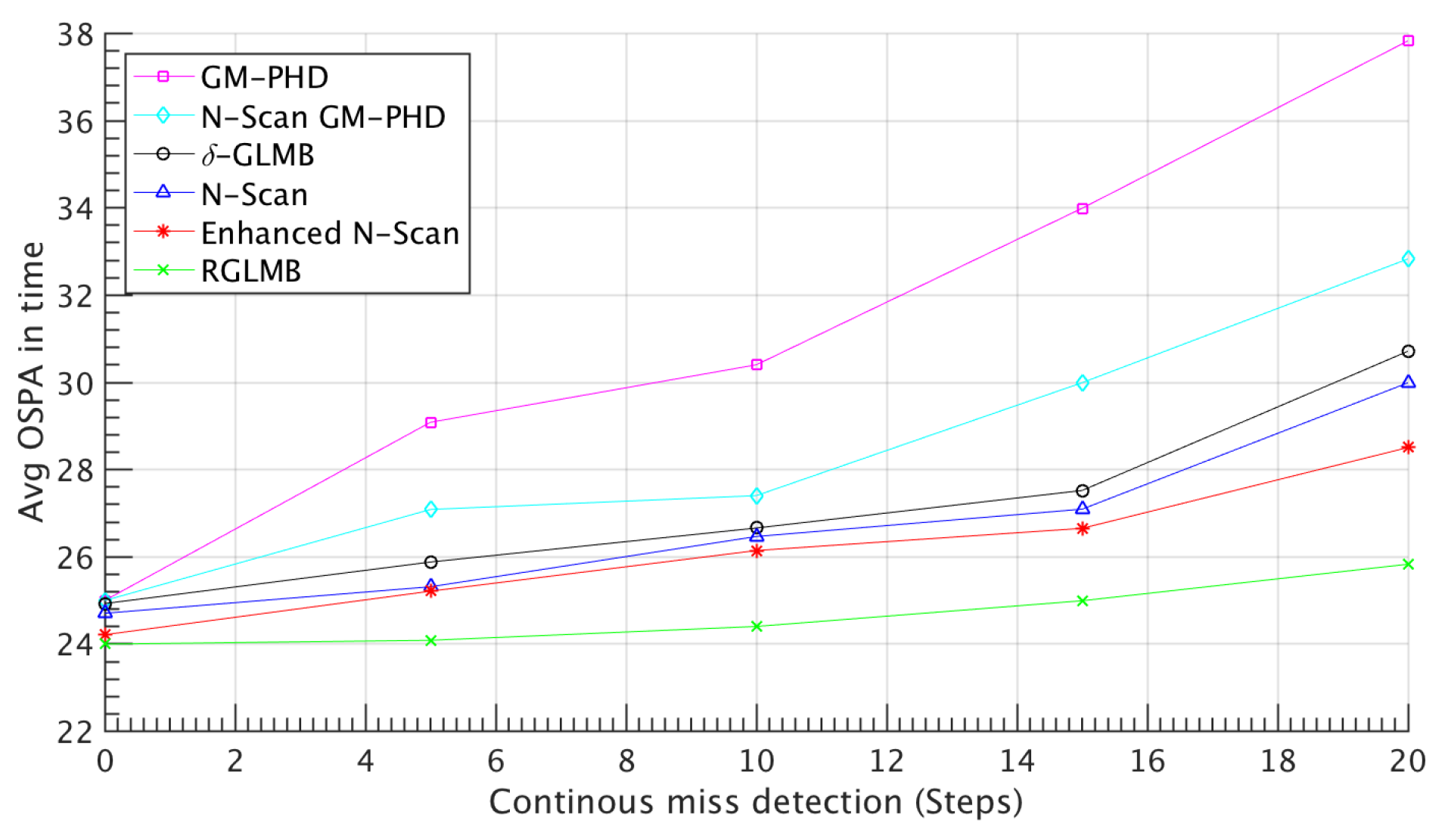
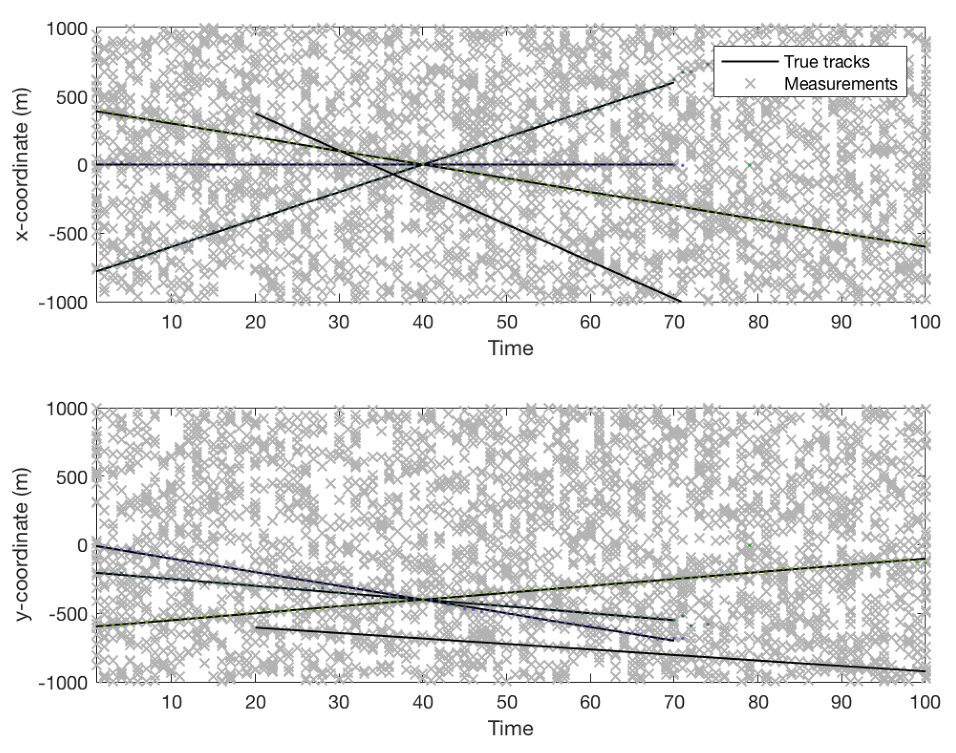
4.1. Simulated Dataset Results

A typical scenario is considered as a set of multi-target trajectories on a two-dimensional region [−1000,1000] m × [−1000,1000] m, as shown in Figure 1.

We begin with a duration of $K=100$ s. The number of targets may change during the time as an outcome of births and deaths. The kinematic target state is a 4D vector which contains planar position and constant velocity (target velocities are constant and may differ from each other) $x_k={[p_{x,k},p_{y,k},{\dot{p}}_{x,k},{\dot{p}}_{y,k}]}^T$. Noisy vectors of the 2D planar position $z_k={[z_{x,k},z_{y,k}]}^T$ show the measurements. The single-target state space model is linear Gaussian with $f_{k|k-1}\left(x_k\right|x_{k-1})=\mathcal{N}(x_k;F_k{x}_{k-1},Q_k)$ and a Gaussian likelihood $g_k\left(z_k\right|x_k)=\mathcal{N}(z_k;H_k{x}_k,R_k)$, where $F,H$ are state and observation transition matrices, respectively, and $R,Q$ are noise matrices which are represented by

$$F_k=\left[\begin{array}{cccc}1& 1& \Delta & \Delta \\ 1& 1& \Delta & \Delta \\ 0& 0& 1& 1\\ 0& 0& 1& 1\end{array}\right],H_k=\left[\begin{array}{cccc}1& 1& 0& 0\\ 1& 1& 0& 0\end{array}\right],Q_k={\sigma }_v^2\left[\begin{array}{cccc}{\displaystyle \frac{{\Delta }^4}{4}}& {\displaystyle \frac{{\Delta }^4}{4}}& {\displaystyle \frac{{\Delta }^3}{2}}& {\displaystyle \frac{{\Delta }^3}{2}}\\ {\displaystyle \frac{{\Delta }^4}{4}}& {\displaystyle \frac{{\Delta }^4}{4}}& {\displaystyle \frac{{\Delta }^3}{2}}& {\displaystyle \frac{{\Delta }^3}{2}}\\ {\displaystyle \frac{{\Delta }^3}{2}}& {\displaystyle \frac{{\Delta }^3}{2}}& {\Delta }^2& {\Delta }^2\\ {\displaystyle \frac{{\Delta }^3}{2}}& {\displaystyle \frac{{\Delta }^3}{2}}& {\Delta }^2& {\Delta }^2\end{array}\right],R_k={\sigma }_{ϵ}^2\left[\begin{array}{cc}1& 1\\ 1& 1\end{array}\right]$$

where $\Delta =1$ s is the sampling period, and ${\sigma }_v=5$ ${\mathrm{ms}}^2$ and ${\sigma }_{ϵ}=10$ m are standard deviations of the process and measurement noise. The survival probability is $P_{S,k}=0.97$ (except the RGM version, for which the probability of survival is adaptive), and the birth model is a Labelled Multi-Bernoulli RFS with parameters ${\pi }_B={\{r_B^{\left(i\right)},p_B^{\left(i\right)}\}}_{i=1}^4$, where $r_B^{\left(i\right)}=0.03$ and $p_B^{\left(i\right)}\left(x\right)=\mathcal{N}(x;m_B^{\left(i\right)},P_B)$ with $m_B^{\left(1\right)}={[0.1,0,0.1,0]}^T$, $m_B^{\left(2\right)}={[400,0,-600,0]}^T$, $m_B^{\left(3\right)}={[-800,0,-200,0]}^T$, $m_B^{\left(4\right)}={[-200,0,800,0]}^T$, $P_B=diag{\left({[10,10,10,10]}^T\right)}^2$. Clutter follows a Poisson RFS, giving an average of 65 false alarms per scan. The $\delta$-GLMB filter is capped at 12,000 components, and results are shown for 100 Monte Carlo trials. The comparison criteria for the methods are fromOptimal Sub-Pattern Assignment (OSPA) [51,52] with a cut-off of $c=100$ and order of $p=1$. The OSPA formulation is calculated as

$$OSP{A}^{c,p}(X_k,\widehat{X_k})={\left[{\displaystyle \frac{1}{|\widehat{X_k}|}}\left(\underset{\pi \in {\Pi }_{|\widehat{X_k}|}}{min}\sum _{i=1}^{|X_k|}{\left(d_c(x^i,{\widehat{x}}^{\pi \left(i\right)})\right)}^p+c^p\times \left(\right|\widehat{X_k}|-|X_k\left|\right)\right)\right]}^{{\displaystyle \frac{1}{p}}}$$

(60)

The results shown for the N-scan method are obtained considering fixed values for N-scan parameters. The length of the history window is $N=5,N_{Init}=3$ and $N_{Surv}=2$.

Figure 2 shows the results for the standard $\delta$-GLMB filter, N-scan $\delta$-GLMB filter, N-scan $\delta$-GLMB filter with enhanced update and prediction steps, and refined $\delta$-GLMB. These results are obtained with a detection rate of $80\%$, and the average OSPA in this situation is shown in

Table 2. AVG OSPA of different methods in 100 filtering iterations.

Method (${\mathit{P}}_{\mathit{D}}=0.8$)	OSPA (AVG) (# of Targets)
GM-PHD [53]	47.46 (5.17)
N-scan GM-PHD [43]	39.71 (5.88)
$\delta$-GLMB	33.4375 (6.13)
N-scan $\delta$-GLMB	31.1589 (6.71)
Enhanced N-scan $\delta$-GLMB	29.4330 (6.94)
Refined N-scan $\delta$-GLMB	27.0017 (7.26)

.

Figure 3 shows the result for different detection probability rates versus the average of OSPA in time. This result shows that the effects of miss detection are decreased using the proposed methods. Notice that in the higher rate of miss detection situation, the proposed methods diverge from the standard $\delta$-GLMB, which shows that the proposed methods operate better in uncertain conditions.

Figure 4 shows the analysis of the methods in different clutter rates, and Figure 5 shows the result in the scenario where some targets are forced to be miss-detected for a certain number of frames in a sequence. The results demonstrate that the proposed N-scan and refined $\delta$-GLMB method improved the estimation performance of the $\delta$-GLMB in uncertain conditions, since the OSPA of the proposed methods decreased compared to the other methods, especially when the uncertainty rate increased. For example, the OSPA distance between our proposed method and other methods obtains a higher value in lower rates of detection, which shows a better performance in uncertain conditions. The proposed refined method also outperforms other methods in the sequenced miss detection. Notice that some proposed methods, like Marginalised $\delta$-GLMB [54], which are recently proposed perform analogously to the $\delta$-GLMB from the aspect of estimation in uncertain conditions. The proposed methods of this paper focus on enhancing the performance of the $\delta$-GLMB filters family; hence, this idea and these methods can be used on other forms of the $\delta$-GLMB.

Figure 6 shows another scenario with a vivid, high amount of uncertainty in the measurements and also dense occlusion in both the X and Y axes. The discussed methods are performed on this scenario, and results are shown in

Table 3. Average OSPA of different methods in 100 filtering iterations for the scenario defined in Figure 6.

Method	OSPA (AVG)
GM-PHD [53]	39.03
N-scan GM-PHD [43]	34.51
$\delta$-GLMB [42]	32.28
N-scan $\delta$-GLMB (ours)	28.67
Enhanced N-scan $\delta$-GLMB (ours)	26.44
Refined N-scan $\delta$-GLMB (ours)	24.10

, which shows the effectiveness of our proposed methods in heavily uncertain conditions.

4.2. Visual Dataset Results

Here, the PETS09-S2L1 and GRAM-RTM [55] datasets are utilised in order to verify the functionality of the proposed methods. We chose PETS09-S2L1 as a dataset, which is crowded with people (presenting a proper multi-object tracking environment) and contains certain obstacles in the scene which cause momentary and continuous occlusions. The GRAM-RTM dataset is chosen because of loads of vehicles crossing in the scene and consequently, a high amount of occlusion. The GRAM-RTM dataset is low-quality, which also causes miss detection. Hence, it is possible to verify the proposed methods’ performance in a challenging environment with uncertainties in the measurement. Figure 7 shows the quality of different methods in sub-samples of the PETS09-S2L1 and GRAM-RTM datasets. As is clear in Figure 7, the $\delta$-GLMB fails to track the targets which are behind the obstacle in the middle of the scene; however, the three other proposed methods show progress in tracking. The scene shown in Figure 7 is a frame where two different objects move from different locations, come across each other, stay for moments (which is mostly miss-detected because of the presence of solid obstacles in the scene), and leave the scene in different directions. The qualitative results shown in Figure 7 show that the proposed methods are more successful in tracking targets than the original $\delta$-GLMB method since they track the targets in more frames and confront the miss-detection effect.

The quantitative results for PETS09-S2L1 and GRAM-RTM are shown in

Table 4. Results of different methods on PETS09-S2L1.

Method	MOTA	MOTP	ReR	FAR	MTR	MOR
GM-PHD [53]	42.62	54.02	0.45	0.12	0.57	0.71
N-scan GM-PHD [43]	46.78	58.49	0.51	0.10	0.46	0.57
$\delta$-GLMB [42]	51.05	63.62	0.57	0.10	0.42	0.64
N-scan $\delta$-GLMB (ours)	54.53	65.28	0.62	0.07	0.34	0.42
Enhanced N-scan $\delta$-GLMB (ours)	55.60	65.91	0.62	0.07	0.34	0.35
Refined N-scan $\delta$-GLMB (ours)	56.79	66.38	0.71	0.05	0.26	0.28

and

Table 5. Results of different methods on GRAM-RTM.

Method	MOTA	MOTP	ReR	FAR	MTR	MOR
GM-PHD [53]	27.91	32.59	0.31	0.17	0.68	0.78
N-scan GM-PHD [43]	31.20	36.17	0.46	0.12	0.56	0.66
$\delta$-GLMB [42]	30.83	37.55	0.48	0.14	0.53	0.64
N-scan $\delta$-GLMB (ours)	35.41	40.06	0.58	0.07	0.46	0.56
Enhanced N-scan $\delta$-GLMB (ours)	36.26	41.74	0.60	0.07	0.41	0.53
Refined N-scan $\delta$-GLMB (ours)	39.32	43.45	0.68	0.04	0.34	0.43

, respectively, where popular CLEAR MOT metrics are used to evaluate the performance of the trackers [56,57]. The MOT metrics used here are MOTA and MOTP. MOTA, or the Multiple Object Tracking Accuracy measure, combines three error sources, false positives, missed targets, and identity switches, calculated as

$$MOTA=1-{\displaystyle \frac{{\sum }_k(FalseNegativ{e}_k+FlasePositiv{e}_k+N{S}_k)}{{\sum }_{k}n{g}_k}}$$

(61)

where k is the frame number and $n{b}_k$ is the number of estimated bounding boxes at frame k. MOTP, or the Multiple Object Tracking Precision measure, is a criterion for how the tracker performs in a situation of misalignment between the annotated and predicted bounding boxes, calculated as

$${\displaystyle \left(\sum _{t\in targets,k}Area(groundTrut{h}_k^t\cap estimate{d}_k^t)/Area(groundTrut{h}_k^t\cup estimate{d}_k^t)\right)/\sum _{k}n{b}_k}$$

(62)

where $n{g}_k$ denotes the number of ground truths at frame k and $N{S}_k$ is the number of target identity switches. The results also contain four other numerical metrics. The Recall Rate (ReR) metric is brought to verify the ability of the filters for true estimations. The False Alarm Rate (FAR) is utilised to investigate the effect of the uncertainty. The Missed Trajectory Rate (MTR) and the Missed Occlusion Rate (MOR) evaluate the amount of improvement for handling occlusion. These criteria are calculated as

$$ReR={\displaystyle \frac{\# \mathrm{true} \mathrm{estimations}}{\# \mathrm{totoal} \mathrm{ground} \mathrm{truth} \mathrm{targets}}},FAR={\displaystyle \frac{\# \mathrm{false} \mathrm{estimations}}{\# \mathrm{total} \mathrm{estimations}}},$$

$$MTR={\displaystyle \frac{\# \mathrm{missed} \mathrm{trajectories}}{\# \mathrm{total} \mathrm{trajectories}}},MOR={\displaystyle \frac{\# \mathrm{missed} \mathrm{occlusions}}{\# \mathrm{total} \mathrm{occlusions}}}$$

As is clear from the results, our proposed methods improve the mentioned considered criteria. The criteria MOTA and MOTP are improved, which shows that the proposed methods improve the tracking accuracy and precision of the other discussed trackers. The criteria ReR, FAR, MTR, and MOR are improved, which are criteria for verifying the performance of the trackers in uncertain conditions. For example, decreasing MTR shows that the number of missed trajectories are significantly decreased in our proposed methods compared with the other verified methods. In total, these results show that utilising the information stored in the history of the filtering performance causes a better performance for trackers. For example, when a person detected in the scene is not detected for a while, knowing that this person existed and moved in a certain direction can help the tracker to expect that the person will be seen again in a rational (due to the history of appearance in the scene) area.

5. Conclusions

In practice, $\delta$-GLMB filter performance may decrease in uncertain conditions due to truncation of informative components which have lost information at the moment of the occurrence of an uncertainty. In this paper, we proposed methods that aim at improving the performance of the filtering via guessing which components occur under the mentioned circumstances and keeping them from being removed from the filtering procedure. The main idea is utilising the information stored in the history of the filtering procedure. We benefit from information stored in the last N iterations of filtering, using it to guess which components are truncating wrongly according to their behaviour during the time of their existence (with regard to the N value). Then we use a survival model and a reward-and-punishment scheme to make sure that a component is confirmed to be truncated or to survive. The performance of the proposed methods is verified via a simulated scenario and multiple conditions in terms of different probabilities of detection, different clutter rates, and a subsequent miss-detection scenario whose targets were forced to be miss-detected for coherent sequenced frames. The proposed methods were compared with the standard $\delta$-GLMB filter, and the results show that the proposed methods outperform it in the presence of random uncertainties.

References

1. Bar, S.Y.; Fortmann, T. Tracking and Data Association. Ph.D. Thesis, Academic Press, Cambridge, UK, 1988. [Google Scholar]
2. Blackman, S.; Popoli, R. Design and Analysis of Modern Tracking Systems (Artech House Radar Library); Artech House: London, UK, 1999. [Google Scholar]
3. Alhadhrami, E.; Seghrouchni, A.E.F.; Barbaresco, F.; Zitar, R.A. Testing Different Multi-Target/Multi-Sensor Drone Tracking Methods Under Complex Environment. In Proceedings of the 2024 International Radar Symposium (IRS), Wroclaw, Poland, 2–4 July 2024; IEEE: Piscataway, NJ, USA, 2024; pp. 352–357. [Google Scholar]
4. Hong, J.; Wang, T.; Han, Y.; Wei, T. Multi-Target Tracking for Satellite Videos Guided by Spatial-Temporal Proximity and Topological Relationships. IEEE Trans. Geosci. Remote Sens. 2025, 63, 5614020. [Google Scholar] [CrossRef]
5. Wang, X.; Li, D.; Wang, J.; Tong, D.; Zhao, R.; Ma, Z.; Li, J.; Song, B. Continuous multi-target tracking across disjoint camera views for field transport productivity analysis. Autom. Constr. 2025, 171, 105984. [Google Scholar] [CrossRef]
6. Reuter, S.; Vo, B.T.; Vo, B.N.; Dietmayer, K. The Labeled Multi-Bernoulli Filter. IEEE Trans. Signal Process. 2014, 62, 3246–3260. [Google Scholar] [CrossRef]
7. Blackman, S.S. Multiple hypothesis tracking for multiple target tracking. IEEE Aerosp. Electron. Syst. Mag. 2004, 19, 5–18. [Google Scholar] [CrossRef]
8. Yang, Y.; Yan, T.; Shen, J.; Sun, G.; Tian, Z.; Ju, W. Multi-Hypothesis Tracking Algorithm for Missile Group Targets. In Proceedings of the 2024 IEEE International Conference on Unmanned Systems (ICUS), Nanjing, China, 18–20 October 2024; IEEE: Piscataway, NJ, USA, 2024; pp. 745–750. [Google Scholar]
9. Yang, Z.; Nie, H.; Liu, Y.; Bian, C. Robust Tracking Method for Small and Weak Multiple Targets Under Dynamic Interference Based on Q-IMM-MHT. Sensors 2025, 25, 1058. [Google Scholar] [CrossRef]
10. Fortmann, T.; Bar-Shalom, Y.; Scheffe, M. Sonar tracking of multiple targets using joint probabilistic data association. IEEE J. Ocean. Eng. 1983, 8, 173–184. [Google Scholar] [CrossRef]
11. Chen, Q.; Wang, P.; Wei, H. An algorithm for multi-target tracking in low-signal-to-clutter-ratio underwater acoustic scenes. AIP Adv. 2024, 14, 105121. [Google Scholar] [CrossRef]
12. Gu, Z.; Cheng, S.; Wang, C.; Wang, R.; Zhao, Y. Robust Visual Localization System With HD Map Based on Joint Probabilistic Data Association. IEEE Robot. Autom. Lett. 2024, 9, 9415–9422. [Google Scholar] [CrossRef]
13. Mahler, R. Random set theory for target tracking and identification. In Data Fusion Hand Book; CRC Press: Boca Raton, FL, USA, 2001. [Google Scholar]
14. Daley, D.J.; Vere-Jones, D. An Introduction to the Theory of Point Processes: Volume II: General Theory and Structure; Springer Science & Business Media: Berlin/Heidelberg, Germany, 2007. [Google Scholar]
15. Forti, N.; Millefiori, L.M.; Braca, P.; Willett, P. Random finite set tracking for anomaly detection in the presence of clutter. In Proceedings of the 2020 IEEE Radar Conference (RadarConf20), Florence, Italy, 21–25 September 2020; IEEE: Piscataway, NJ, USA, 2020; pp. 1–6. [Google Scholar]
16. Yao, X.; Qi, B.; Wang, P.; Di, R.; Zhang, W. Novel Multi-Target Tracking Based on Poisson Multi-Bernoulli Mixture Filter for High-Clutter Maritime Communications. In Proceedings of the 2024 12th International Conference on Information Systems and Computing Technology (ISCTech), Xi’an, China, 8–11 November 2024; IEEE: Piscataway, NJ, USA, 2024; pp. 1–7. [Google Scholar]
17. Si, W.; Wang, L.; Qu, Z. Multi-target tracking using an improved Gaussian mixture CPHD Filter. Sensors 2016, 16, 1964. [Google Scholar] [CrossRef]
18. Li, C.; Bao, Q.; Pan, J. Multi-target Tracking Method of Non-cooperative Bistatic Radar System Based on Improved PHD Filter. In Proceedings of the 2024 Photonics & Electromagnetics Research Symposium (PIERS), Chengdu, China, 21–25 April 2024; IEEE: Piscataway, NJ, USA, 2024; pp. 1–7. [Google Scholar]
19. Hoseinnezhad, R.; Vo, B.N.; Vo, B.T. Visual tracking in background subtracted image sequences via multi-Bernoulli filtering. IEEE Trans. Signal Process. 2013, 61, 392–397. [Google Scholar] [CrossRef]
20. Wu, W.; Sun, H.; Zheng, M.; Huang, W. Target Tracking with Random Finite Sets; Springer: Berlin/Heidelberg, Germany, 2023. [Google Scholar]
21. Lee, C.S.; Clark, D.E.; Salvi, J. SLAM with dynamic targets via single-cluster PHD filtering. IEEE J. Sel. Top. Signal Process. 2013, 7, 543–552. [Google Scholar] [CrossRef]
22. Zhang, Y.; Li, Y.; Li, S.; Zeng, J.; Wang, Y.; Yan, S. Multi-target tracking in multi-static networks with autonomous underwater vehicles using a robust multi-sensor labeled multi-Bernoulli filter. J. Mar. Sci. Eng. 2023, 11, 875. [Google Scholar] [CrossRef]
23. Chen, J.; Xie, Z.; Dames, P. The semantic PHD filter for multi-class target tracking: From theory to practice. Robot. Auton. Syst. 2022, 149, 103947. [Google Scholar]
24. Jeong, T. Particle PHD filter multiple target tracking in sonar image. IEEE Trans. Aerosp. Electron. Syst. 2007, 43, 409–416. [Google Scholar]
25. Zeng, Y.; Wang, J.; Wei, S.; Zhang, C.; Zhou, X.; Lin, Y. Gaussian mixture probability hypothesis density filter for heterogeneous multi-sensor registration. Mathematics 2024, 12, 886. [Google Scholar] [CrossRef]
26. Liang, G.; Zhang, B.; Qi, B. An augmented state Gaussian mixture probability hypothesis density filter for multitarget tracking of autonomous underwater vehicles. Ocean Eng. 2023, 287, 115727. [Google Scholar]
27. Leach, M.J.; Sparks, E.P.; Robertson, N.M. Contextual anomaly detection in crowded surveillance scenes. Pattern Recognit. Lett. 2014, 44, 71–79. [Google Scholar]
28. Blair, A.; Gostar, A.K.; Bab-Hadiashar, A.; Li, X.; Hoseinnezhad, R. Enhanced Multi-Target Tracking in Dynamic Environments: Distributed Control Methods Within the Random Finite Set Framework. arXiv 2024, arXiv:2401.14085. [Google Scholar]
29. Meißner, D.A.; Reuter, S.; Strigel, E.; Dietmayer, K. Intersection-Based Road User Tracking Using a Classifying Multiple-Model PHD Filter. IEEE Intell. Transport. Syst. Mag. 2014, 6, 21–33. [Google Scholar]
30. Zhang, Y.; Zhang, B.; Shen, C.; Liu, H.; Huang, J.; Tian, K.; Tang, Z. Review of the field environmental sensing methods based on multi-sensor information fusion technology. Int. J. Agric. Biol. Eng. 2024, 17, 1–13. [Google Scholar]
31. Gruden, P.; White, P.R. Automated extraction of dolphin whistles—A sequential Monte Carlo probability hypothesis density approach. J. Acoust. Soc. Am. 2020, 148, 3014–3026. [Google Scholar] [CrossRef] [PubMed]
32. Rezatofighi, S.H.; Gould, S.; Vo, B.N.; Mele, K.; Hughes, W.E.; Hartley, R. A multiple model probability hypothesis density tracker for time-lapse cell microscopy sequences. In Proceedings of the International Conference on Information Processing in Medical Imaging, Asilomar, CA, USA, 28 June–3 July 2013; Springer: Berlin/Heidelberg, Germany, 2013; pp. 110–122. [Google Scholar]
33. Ben-Haim, T.; Raviv, T.R. Graph neural network for cell tracking in microscopy videos. In Proceedings of the European Conference on Computer Vision, Tel Aviv, Israel, 23–27 October 2022; Springer: Berlin/Heidelberg, Germany, 2022; pp. 610–626. [Google Scholar]
34. Kim, D.Y. Multi-Bernoulli filtering for keypoint-based visual tracking. In Proceedings of the 2016 International Conference on Control, Automation and Information Sciences (ICCAIS), Ansan, Republic of Korea, 27–29 October 2016; IEEE: Piscataway, NJ, USA, 2016; pp. 37–41. [Google Scholar]
35. Baker, L.; Ventura, J.; Langlotz, T.; Gul, S.; Mills, S.; Zollmann, S. Localization and tracking of stationary users for augmented reality. Vis. Comput. 2024, 40, 227–244. [Google Scholar] [CrossRef]
36. Mahler, R.P. Advances in Statistical Multisource-Multitarget Information Fusion; Artech House: London, UK, 2014. [Google Scholar]
37. Mahler, R.P. Multitarget Bayes filtering via first-order multitarget moments. IEEE Trans. Aerosp. Electron. Syst. 2003, 39, 1152–1178. [Google Scholar] [CrossRef]
38. Mahler, R. PHD filters of higher order in target number. IEEE Trans. Aerosp. Electron. Syst. 2007, 43, 1523–1543. [Google Scholar] [CrossRef]
39. Vo, B.N.; Vo, B.T.; Pham, N.T.; Suter, D. Joint detection and estimation of multiple objects from image observations. IEEE Trans. Signal Process. 2010, 58, 5129–5141. [Google Scholar] [CrossRef]
40. Vo, B.N.; Vo, B.T.; Phung, D. Labeled random finite sets and the Bayes multi-target tracking filter. IEEE Trans. Signal Process. 2014, 62, 6554–6567. [Google Scholar] [CrossRef]
41. Vo, B.T.; Vo, B.N. Labeled random finite sets and multi-object conjugate priors. IEEE Trans. Signal Process. 2013, 61, 3460–3475. [Google Scholar] [CrossRef]
42. Liu, Z.; Zheng, D.; Yuan, J.; Chen, A.; Li, H.; Zhou, C.; Chen, W.; Liu, Q. δ-GLMB Filter Based on Multiple Model Multiple Hypothesis Tracking. In Proceedings of the 2022 14th International Conference on Signal Processing Systems (ICSPS), online, 18–20 November 2022; IEEE: Piscataway, NJ, USA, 2022; pp. 249–258. [Google Scholar]
43. Yazdian-Dehkordi, M.; Azimifar, Z. Novel N-scan GM-PHD-based approach for multi-target tracking. IET Signal Process. 2016, 10, 493–503. [Google Scholar] [CrossRef]
44. Mahler, R.P. Statistical Multisource-Multitarget Information Fusion; Artech House, Inc.: London, UK, 2007. [Google Scholar]
45. Vo, B.N.; Ma, W.K. The Gaussian mixture probability hypothesis density filter. IEEE Trans. Signal Process. 2006, 54, 4091. [Google Scholar] [CrossRef]
46. Sepanj, M.H.; Azimifar, Z. N-scan δ-generalized labeled multi-bernoulli-based approach for multi-target tracking. In Proceedings of the Artificial Intelligence and Signal Processing Conference (AISP), Shiraz, Iran, 25–27 October 2017; IEEE: Piscataway, NJ, USA, 2017; pp. 103–106. [Google Scholar]
47. Miller, M.L.; Stone, H.S.; Cox, I.J. Optimizing Murty’s ranked assignment method. IEEE Trans. Aerosp. Electron. Syst. 1997, 33, 851–862. [Google Scholar] [CrossRef]
48. Murty, K.G. Letter to the editor—An algorithm for ranking all the assignments in order of increasing cost. Oper. Res. 1968, 16, 682–687. [Google Scholar]
49. Punchihewa, Y.G.; Vo, B.T.; Vo, B.N.; Kim, D.Y. Multiple Object Tracking in Unknown Backgrounds With Labeled Random Finite Sets. IEEE Trans. Signal Process. 2018, 66, 3040–3055. [Google Scholar] [CrossRef]
50. Yazdian-Dehkordi, M.; Azimifar, Z. Refined GM-PHD tracker for tracking targets in possible subsequent missed detections. Signal Process. 2015, 116, 112–126. [Google Scholar]
51. Schuhmacher, D.; Vo, B.T.; Vo, B.N. A consistent metric for performance evaluation of multi-object filters. IEEE Trans. Signal Process. 2008, 56, 3447–3457. [Google Scholar] [CrossRef]
52. Tang, T.; Wang, P.; Zhao, P.; Zeng, H.; Chen, J. A novel multi-target TBD scheme for GNSS-based passive bistatic radar. IET Radar Sonar Navig. 2024, 18, 2497–2512. [Google Scholar] [CrossRef]
53. Liu, J.; Wu, Z.; Zhao, J.; Han, X. Improved GM-PHD Filter for Multi-target Tracking with Dense Clutter and Low Detection Probability. In Proceedings of the 2024 43rd Chinese Control Conference (CCC), Kunming, China, 28–31 July 2024; IEEE: Piscataway, NJ, USA, 2024; pp. 3505–3510. [Google Scholar]
54. Vo, B.N.; Vo, B.T.; Hoang, H.G. An efficient implementation of the generalized labeled multi-Bernoulli filter. IEEE Trans. Signal Process. 2017, 65, 1975–1987. [Google Scholar] [CrossRef]
55. Guerrero-Gomez-Olmedo, R.; Lopez-Sastre, R.J.; Maldonado-Bascon, S.; Fernandez-Caballero, A. Vehicle Tracking by Simultaneous Detection and Viewpoint Estimation. In Proceedings of the IWINAC 2013, Mallorca, Spain, 10–14 June 2013; Part II, LNCS 7931. pp. 306–316. [Google Scholar]
56. Bernardin, K.; Stiefelhagen, R. Evaluating multiple object tracking performance: The CLEAR MOT metrics. J. Image Video Process. 2008, 2008, 246309. [Google Scholar] [CrossRef]
57. Putra, H.; Nuha, H.H.; Irsan, M.; Putrada, A.G.; Hisham, S.B.I. Object Tracking in Surveillance System Using Particle Filter and ACF Detection. In Proceedings of the 2024 International Conference on Decision Aid Sciences and Applications (DASA), Hybrid, Bahrain, 11–12 December 2024; IEEE: Piscataway, NJ, USA, 2024; pp. 1–7. [Google Scholar]
58. Sepanj, H.; Fieguth, P. Context-Aware Augmentation for Contrastive Self-Supervised Representation Learning. J. Comput. Vis. Imaging Syst. 2023, 9, 4–7. [Google Scholar]
59. Sepanj, H.; Fieguth, P. Aligning Feature Distributions in VICReg Using Maximum Mean Discrepancy for Enhanced Manifold Awareness in Self-Supervised Representation Learning. J. Comput. Vis. Imaging Syst. 2024, 10, 13–18. [Google Scholar]
60. Sepanj, M.H.; Fiegth, P. SinSim: Sinkhorn-Regularized SimCLR. arXiv 2025, arXiv:2502.10478. [Google Scholar]
61. Sepanj, M.H.; Ghojogh, B.; Fieguth, P. Self-Supervised Learning Using Nonlinear Dependence. arXiv 2025, arXiv:2501.18875. [Google Scholar]
Figure 1. Multiple trajectories on the XY plane which are inputs for tracking simulation procedure. Start/stop positions for each track are shown with o/ Δ . Notice that at the same time, there are at most 10 targets in the system according to different times of birth and death of targets. The targets are occluded, and they cross each other in certain locations shown in the figure.
Bdcc 09 00084 g001
Figure 2. The figure shows OSPA of different methods in 100 filtering iterations (100 Monte Carlo trials). P D = 0.80 , and 65 clutter per frame is used. As is clear in the figure, the areas under the lines of the proposed methods are lower than the δ -GLMB method, which results in a lower average of OSPA in time and consequently shows a better result obtained.
Bdcc 09 00084 g002
Figure 3. Different probabilities of detection (100 Monte Carlo trials). As is clear in the figure, the proposed methods outperform the δ -GLMB method in the presence of miss detection. With higher rates of miss detection (lower probability of detection), the divergence between different methods increases, which shows the power of the proposed method in more uncertain conditions like the presence of clutter.
Bdcc 09 00084 g003
Figure 4. Different clutter per frame rates with probability of detection of 0.95 (100 Monte Carlo trials). As is clear in the figure, the proposed methods outperform the δ -GLMB method in the presence of clutter. With higher rates of clutter, the divergence between different methods increases, which shows the power of the proposed method in more uncertain conditions like the presence of miss detection.
Bdcc 09 00084 g004
Figure 5. Different forced consequent miss detection rates with P D = 0.95 (100 Monte Carlo trials). This figure shows the examination of the proposed method in a condition where miss detection happens consequently; as is clear in the figure, the refined GLMB out performs the other methods.
Bdcc 09 00084 g005
Figure 6. Multiple trajectories in X-Time and Y-Time planes, which are highly occluded, and the amount of uncertainty in the measurements is clearly intense.
Bdcc 09 00084 g006
Figure 7. Results on PETS09-S2L1 (first row) and GRAM-RTM (Urban1) (second row). For simplicity, just two target trajectories are drawn in the pictures. (First column) Trajectory for δ -GLMB method. (Second column) Trajectory for N-scan method. (Third column) Trajectory for enhanced method. (Fourth column) Trajectory for refined δ -GLMB.
Bdcc 09 00084 g007