Article

Analysis of China’s High-Speed Railway Network Using Complex Network Theory and Graph Convolutional Networks

1
Centre for Computational Engineering Sciences, Cranfield University, Cranfield, Bedfordshire MK43 0AL, UK
2
Institute of Geographic Sciences and Natural Resources Research, Chinese Academy of Sciences, Beijing 100101, China
*
Author to whom correspondence should be addressed.
Big Data Cogn. Comput. 2025, 9(4), 101; https://doi.org/10.3390/bdcc9040101
Submission received: 11 March 2025 / Revised: 10 April 2025 / Accepted: 11 April 2025 / Published: 16 April 2025

Abstract

This study investigated the characteristics and functionalities of China’s High-Speed Railway (HSR) network based on Complex Network Theory (CNT) and Graph Convolutional Networks (GCN). First, complex network analysis was applied to provide insights into the network’s fundamental characteristics, such as small-world properties, efficiency, and robustness. Then, this research developed three novel GCN models to identify key nodes, detect community structures, and predict new links. Findings from the complex network analysis revealed that China’s HSR network exhibits a typical small-world property, with a degree distribution that follows a log-normal pattern rather than a power law. The global efficiency indicator suggested that stations are typically connected through direct routes, while the local efficiency indicator showed that the network performs effectively within local areas. The robustness study indicated that the network can quickly lose connectivity if key nodes fail, though it showed an ability initially to self-regulate and has partially restored its structure after disruption. The GCN model for key node identification revealed that the key nodes in the network were predominantly located in economically significant and densely populated cities, positively contributing to the network’s overall efficiency and robustness. The community structures identified by the integrated GCN model highlight the economic and social connections between official urban clusters and the communities. Results from the link prediction model suggest the necessity of improving the long-distance connectivity across regions. Future work will explore the network’s socio-economic dynamics and refine and generalise the GCN models.

1. Introduction

The complex network approach is recognised for its ability to uncover the statistical characteristics and measurements of networks, which are pivotal in assessing and enhancing railway systems, particularly in the analysis of intricate network datasets. For instance, a study of the Indian Railway Network [1] confirmed the presence of small-world characteristics and exponential distributions of node degrees and edge weights, which are commonly observed in railway networks. It also identified the most critical stations and explored the correlations between traffic and network topology. The work of [2] introduced the complex network method to the study of physical railway structures and operational strategies for analysing network efficiency. Its case study results indicate that the key stations identified in the railway network play a significant role in enhancing overall network efficiency. Additionally, the study of [3] proposed a multi-layer complex network-based approach for calculating key indicators to assess node importance and to identify critical track sections.
However, most existing studies focus on analysing the current, static features of a network and do not explore its dynamics, such as predicting link formations and network patterns [4,5,6,7]. While Complex Network Theory (CNT) provides a valuable insight into railway network analysis, its constraints are evident when confronted with extensive and varied network datasets [8,9]. The CNT methods often demand substantial computation and may be too generalised to effectively address the complexities of real-world scenarios.
To address these challenges, this study introduces a novel method that combines Graph Convolutional Network (GCN) models with traditional CNT to improve the analysis of railway network dynamics. This method considers both network structures and intrinsic characteristics, therefore enhancing the prediction accuracy and applicability. A case study on China’s High-Speed Railway (HSR) network was conducted to demonstrate the effectiveness of the approach. The primary objective of this study was to explore whether integrating GCN models with complex network indicators can effectively capture both the topological and functional characteristics of large-scale railway systems. By doing so, this approach aims to uncover critical patterns in node importance, community organisation, and potential connectivity, which are essential for improving transport planning, robustness, and adaptability. The broader contribution lies in demonstrating how modern deep learning techniques can complement traditional network science to support strategic analysis and inform the future development of national-scale transportation systems.
The remainder of this paper is structured as follows: Section 2 reviews state-of-the-art railway network analysis techniques. Section 3 describes the data and methodologies used for complex network analysis. Section 4 presents the research findings. Section 5 discusses the results and limitations, and Section 6 concludes the study.

2. Literature Review

2.1. Railway Network Analysis Based on CNT and GCNs

In the analysis of railway networks using Complex Network Theory (CNT), most studies have primarily focused on examining the network’s static features. For instance, in work [4], the authors highlighted the core–periphery structure and the small-world and scale-free characteristics of China’s railway network while overlooking the network dynamics. Similarly, research [5] did not consider the forecasting and optimisation of potential future connections, which are crucial for enhancing the network’s operational efficiency and resilience. The research in [6] analyses the structure of Iran’s railway network and emphasises the need for optimisation, while the study presented in [7] provides valuable insights into the socio-economic relationships within the railway network. Neither study explored potential performance improvements through predictive modelling of new connections.
Overall, these studies demonstrate the versatility and applicability of CNT in the analysis of railway systems, but limitations remain, particularly in network dynamics analysis and prediction. Moreover, robustness assessment can pinpoint existing risk areas in the network [10,11]. There remains a scarcity of systematic and methodological research on the robustness analysis of railway networks. Given its effectiveness and adaptability, GCNs [12] have the potential to overcome these constraints. Compared to traditional machine learning methods, such as random forest [13], support vector machines (SVM) [14], and conventional artificial neural networks (ANNs) [15], GCNs are particularly suitable for analysing complex networks like railway systems. Unlike traditional approaches that typically treat observations as independent and identically distributed, GCNs inherently leverage graph structures by propagating node-level information through edges, effectively capturing the interdependencies among nodes and enhancing performance in node classification, community detection, and link prediction tasks. Moreover, GCNs offer more accurate analysis and forecasting of railway network dynamics and patterns.
The work in [16] presented a replicable Graph Neural Network benchmarking framework, demonstrating its efficiency in handling complex datasets. The authors in [17] introduced two metrics to predict the potential performance advantages of graph-aware models. The framework proposed in [18] aims to identify the most suitable Graph Neural Network architecture. The GNNLens tool, introduced in [19], focuses on identifying incorrect predictions. GNNExplainer, which was developed in [20], provides both predictions and explanations. In relation to railway analysis, the HetGNN model introduced by [21] is employed to examine train delays, demonstrating the capability of Graph Neural Networks in addressing practical operations. A graphical long short-term memory neural network (G-LSTM) was developed in [22] to assess and forecast the health status of the railway station equipment, enhancing the effectiveness and accuracy of railway equipment management. A multi-view graph attention network model was proposed in [23], achieving high accuracy in forecasting railway traffic. The use of Graph Neural Networks complements CNT in analysing railway systems, providing comprehensive support for optimising railway networks and managing risks.

2.2. The Two Key Topics

In research [24], two specific functions based on CNT—community detection and link prediction—were proposed. The community detection function identifies potential sub-networks within a complex network, while the findings in [25] show that sub-networks enhance comprehension of a network and help identify the characteristics of different network types. Various techniques are available for detecting railway network communities, such as betweenness centrality and modularity maximisation algorithms [26]. The betweenness centrality algorithm detects communities by iteratively removing edges based on centrality values, while the modularity maximisation algorithm partitions communities using the modularity metric to assess effectiveness.
Link prediction methods generally fall into two categories, i.e., learning-based prediction and similarity-based prediction. Learning-based methods employ classification techniques, such as decision trees, Adaboost, and Markov chains [27,28] to forecast the likelihood of links based on node properties. However, feature selection and accuracy evaluation pose significant challenges in practice. Similarity-based methods, including the Jaccard coefficient [29], the Adamic–Adar index [30], and preferential attachment [31], predict links based on node similarity. Relying solely on node similarity is yet insufficient for accurate railway network link prediction. The Graph Neural Network approach addresses these limitations by aggregating the information from nodes, edges, and their neighbours through message passing.
This study aims to develop Graph Convolutional Network models, a variant of Graph Neural Networks, for community detection and link prediction of China’s railway network, to provide a deeper understanding of network features and structure, and to offer a general approach for railway network analysis.

3. Methodology

This study analyses China’s High-Speed Railway (HSR) network using Complex Network Theory (CNT) and Graph Convolutional Networks (GCN). First, the datasets, including train schedules, station information, connections, and timetables, are scraped from the China Railway website. Stations within the same city are consolidated into a single node. The direction of railway connections was not considered due to the bidirectional nature of China’s HSR travel. The key characteristics of the HSR network were summarised, as shown in Table 1, after preprocessing.
Figure 1 presents the structural layout of China’s High-Speed Railway (HSR) network that was used in this study. Each node denotes a city with at least one HSR station, and each edge represents a direct rail connection. Several representative cities across different regions (e.g., Beijing, Shanghai, Guangzhou, Chengdu, Wuhan, Shenzhen, Urumqi, and Harbin) are highlighted to illustrate the network’s geographical coverage and complexity.
Then, complex network indicators (which are defined in Appendix A) were computed to provide insights into the network’s fundamental characteristics. Here, global efficiency and local efficiency were used to measure the network’s transmission capacity, while the assortativity coefficient and network density revealed connectivity patterns and growth potential. The network’s robustness was analysed using the largest strongly connected component proportion, largest weakly connected component proportion, average clustering coefficient, and global efficiency metrics as 10 % , 20 % , 40 % , 50 % , 60 % , and 80 % nodes were gradually removed. Next, a Graph Convolutional Network (GCN) model with a three-layer structure, modulated by the ReLU activation function [12,32], was developed to identify key nodes. The model takes, as input, a node vector with features that include the node degree, betweenness centrality, closeness centrality, and node elasticity, which are then convolved into sixteen hidden features before outputting the node importance. Finally, two additional novel GCN models (which are detailed in the following sections) were developed for community detection and link prediction, respectively.

3.1. Community Detection

GCNs can capture intricate connections and extract the crucial information between network nodes [33]. This research develops an integrated model based on GCNs and clustering algorithms for community detection. A GCN model was developed to generate latent node features and encode the node location and role within a network, which are then used by K-Means [34] and X-Means [35] algorithms for clustering. The GCN model has a three-layer structure, with the Dropout technique being applied to prevent overfitting. Dropout randomly deactivates a subset of neurons during training, which prevents the model from becoming overly reliant on specific features and encourages the learning of more generalisable and robust representations.
Input Feature Construction. Each node is represented by a four-dimensional vector composed of degree centrality, betweenness centrality, closeness centrality, and the clustering coefficient. These features reflect each node’s structural role and importance, and they also serve as the input to the GCN. This approach enables the model to capture both the structural representation and node-level properties of the network.
GCN Architecture. The GCN consists of three graph convolutional layers, each of which are followed by a ReLU activation. The hidden representation has a dimension of 16. Dropout with a rate of 0.5 is applied between layers to prevent overfitting. The propagation rule is as follows:
H ( l + 1 ) = σ ( D ˜ 1 / 2 A ˜ D ˜ 1 / 2 H ( l ) W ( l ) ) ,
where A ˜ = A + I is the adjacency matrix with self-loops, D ˜ is its degree matrix, H ( 0 ) is the input feature matrix, and σ denotes the ReLU activation function.
Optimisation Objective. The loss function Φ ( C ) is computed based on community conductance, which measures the cohesion of a community by a ratio between the number of edges within a community, e intra ( C ) , and the number of edges from other communities to the community, e inter ( C ) :
Φ ( C ) = e inter ( C ) 2 · e intra ( C ) + e inter ( C ) .
In this context, Φ ( C ) evaluates the quality of community C, where a lower value indicates tighter intra-community connectivity and fewer inter-community connections. The final objective is to minimise the total loss L, which is defined as the sum of conductance across all communities C :
L = C C Φ ( C ) .
The loss function reinforces the connectivity within a community while disregarding the inter-communities.
Training and Clustering. The model is trained using the Adam optimiser with a learning rate of 0.01 for 200 epochs. Upon convergence, node embeddings are clustered using the K-Means algorithm. The number of communities is empirically set to 19 based on modularity maximisation and geographic interpretability. This setting balances modularity optimisation with the number of meaningful regional clusters, as community counts below or above this value either under-cluster or fragment core regions excessively.

3.2. Link Prediction

This study developed a novel link prediction model by integrating Graph Attention Networks (GATs) [36] and Variational Graph Autoencoder (VGAE) [37]. In this model, the GAT layer generates the means and log-variances of node representations, which are then used in the reparameterisation process of the VGAE model. In the VGAE model, its original GCN component is replaced with a GAT encoder, which is then combined with an inner product decoder, to capture the latent features of nodes and improve link prediction accuracy.
Model Overview. The model consists of a GAT-based encoder, a reparametrisation module, and an inner-product decoder. The encoder produces two node-level representations, the mean vector μ and the log-variance vector log σ 2 , from which latent variables z are sampled using the reparametrisation trick. The latent variable z refers to a node-level vector representation in the latent space.
Latent Representation Learning. We used two layers of GATs to extract local structural representations. These layers learn the attention coefficients between connected nodes, yielding μ and log σ 2 . The latent embedding z is then obtained by sampling from a Gaussian distribution:
z = μ + ϵ · σ , ϵ N ( 0 , I ) ,
where σ = exp ( 0.5 · log σ 2 ) . This allows for stochastic learning while maintaining backpropagation compatibility.
Edge Probability Decoding. The decoder computes the probability of an edge between a node pair ( i , j ) using an inner product decoder: p i j = σ ( z i T z j ) , where σ is the sigmoid function. Here, z i and z j denote the latent vectors of nodes i and j, and their inner product reflects their similarity in the latent space. A higher inner product corresponds to a higher likelihood of an edge.
Its loss function combines Kullback–Leibler (KL) divergence and binary cross (BC) entropy to balance model overfitting and accuracy, as shown below:
L = K L + B C ,
K L = 1 2 i = 1 N 1 + log ( σ i 2 ) μ i 2 σ i 2 ,
B C = [ y log ( p ) + ( 1 y ) log ( 1 p ) ] ,
where μ , log ( σ i 2 ) , N, y, and p refer to the node mean, node log-variance, number of nodes in the network, observed edge label, and predicted edge probability, respectively. The KL divergence ensures that the distribution of nodes learned does not deviate excessively from the prior distribution, while the BC term compares the observed edge labels (0 or 1) with the predicted probabilities p.
Training Strategy. The model is trained for 200 epochs using the Adam optimiser with a learning rate of 0.01. In each epoch, we sample an equal number of negative links as positive ones to form balanced mini-batches. Early stopping is applied with a patience of 10 epochs to prevent overfitting.
Post-processing and Filtering. After training, all of the unobserved links were ranked by predicted probability. To ensure practical and interpretable recommendations, we applied a filtering process that excludes links within the same existing railway route and those connecting isolated low-degree nodes. Additionally, a Random Forest classifier was trained using topological features (e.g., the node degree and clustering coefficient) to further refine predicted links. Only links with predicted probability above 0.5 and deemed to be informative by the classifier were visualised in the final results.

4. Results

4.1. The Complex Network Characteristics of China’s HSR Network

Table 1 shows that China’s HSR network is a typical small-world network with C > > C R a n d o m and L L Random , where the nodes are closely connected with relatively short distances. In a high-speed railway network, this structure allows geographically distant cities to be connected with only a few transits, boosting the network’s functional efficiency and fostering economic and social connections. Table 2 highlights the top 20 key nodes by degree in China’s HSR network, while Figure 2a,b compare the spatial distribution of the key nodes with economically and demographically dense cities on the Chinese map. This comparison illustrates the urban development patterns and the impact of the railway network on urban growth.
The degree distribution is shown in Figure 3a with a mean degree of 4.8. Figure 3b,c show the cumulative degree distribution and its log–log scale, indicating that the degree distribution does not follow a power law but rather a log-normal distribution. This implies that the network exhibits a hierarchical arrangement, with most cities having moderate connections, while only a few hub cities possess significantly higher connectivity.
Table 3 presents the measured network efficiencies. The global efficiency indicates that the stations are typically connected through direct routes, reducing travel times and costs. This aligns with China’s HSR system, which provides fast connections between economic hubs in the eastern and western regions. The high local efficiency implies that the network performs effectively within local areas or city clusters, demonstrating high redundancy and robustness. This underscores the effective optimisation of the HSR network at the regional level, ensuring the continuity of service even during local disruptions. The assortativity coefficient indicates a tendency for nodes within the network to connect with other nodes of similar degrees. This uniformity in node connectivity, simplifying the network structure and improving operational efficiency, is essential for network stability. The low network density reveals that the HSR network is widespread but has limited connections, suggesting that the network has considerable capacity for future expansion.
Resilience in complex networks refers to the system’s capacity to maintain connectivity and functionality under node failures or external disruptions. In this study, we adopted random node removal (i.e., random attacks) to evaluate the baseline robustness of the HSR network. This approach mimics unpredictable events, such as natural disasters, technical failures, or random malfunctions, which occur without strategic targeting. Although targeted attacks on critical nodes can offer complementary insights, our focus is to simulate generalised disturbances that may arise in real-world scenarios. This methodology follows standard practices in robustness analysis [38,39]. The resilience of the network is studied by simulating random attacks on nodes. Three metrics, i.e., the largest connected component proportion, average clustering coefficient, and global efficiency, were used to evaluate the resulting changes in the network, as shown in Figure 4.
The above figure shows that the largest connected component proportion diminished rapidly as more nodes were removed, suggesting that the network can quickly lose connectivity if key nodes fail. The initial variation in the clustering coefficient indicates the network’s ability to self-regulate and partially restore its structure following a disruption. Interestingly, the global efficiency of the network initially improves as more nodes are removed, reflecting a temporary increase in efficiency due to the removal of peripheral nodes, which reduces the average shortest path lengths among remaining hubs. Overall, China’s HSR network exhibits resilience and adaptation in response to disruptions. Implementing effective improvement strategies and contingency plans is crucial for maintaining network stability.

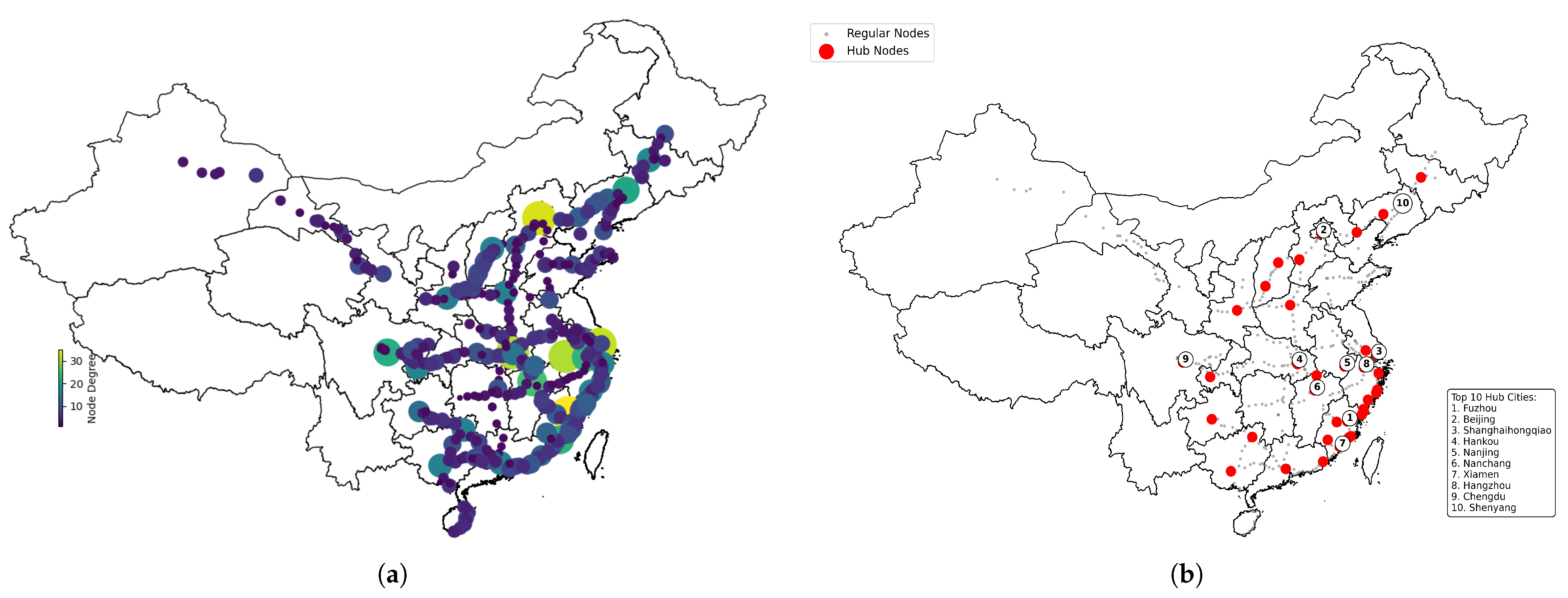
4.2. Key Node Detection

The importance score for each station is predicted by the GCN model, which is listed by rank in Table 4 and mapped onto the Chinese map in Figure 5.
From the table, Fuzhou, Shanghai Hongqiao, and Beijing emerged as the most pivotal nodes, which is consistent with their geographical positions and economic roles in China, while nodes such as Nanjing, Hangzhou, and Xiamen were important as capital cities or local economic hubs. Figure 5 shows that the primary nodes are mainly located in the eastern and central regions of China, especially in the Yangtze River Basin and the Pearl River Delta. These areas are the most vibrant economically in China, and they are characterised by significant urbanisation and economic operations that require well-functioning transportation systems. There are only a limited number of nodes in the western region, which may be due to the region’s economic underdevelopment and low population density. However, this does not imply that well-functioning systems are unnecessary in these regions. On the contrary, improving railway accessibility in the western region is essential for promoting national cohesion and reducing development disparities. The sparse distribution of key nodes in these areas may reflect insufficient infrastructure rather than a lack of necessity. This distribution also highlights the disparity in China’s HSR network development, which should be addressed through targeted policies and investments.
Compared to the conventional hub cities in Figure 2b, which are predominantly clustered in the eastern and central regions of China (which is in line with the country’s economic dynamics and population distribution), the key nodes identified by the GCN model underscore their importance in improving the resilience and effectiveness of the network. Beijing, Shanghai (Hongqiao), and Guangzhou are included in both perspectives, indicating that these urban areas serve not only as major economic and demographic hubs, but also as key structural nodes within the network. Conversely, the cities, including Fuzhou and Nanchang, ranked high by the GCN model and degree distribution did not appear among the conventional hub cities.

4.3. Community Detection and Analysis

The integrated model, which combines GCNs and clustering algorithms, identifies 19 communities, as shown in Figure 6. These communities were identified using the K-Means clustering algorithm applied to the node embeddings produced by the trained GCN model. The number of clusters was set to k = 19 based on empirical observations that align with regional and functional divisions in China’s railway system. This setting provides well-separated community structures that facilitate both visualisation and interpretability.
The figures show clusters of varying sizes and density distributions, reflecting differences in interconnectedness and efficiency. The communities represented by Beijing, Shanghai, and Guangzhou are positioned at the core of the network, which is consistent with their status as major urban hubs. These key urban areas are visually highlighted with red circles in Figure 6 to emphasise their central role. In contrast, communities in the mid-west region exhibited a smaller and more dispersed distribution, highlighting disparities in transportation development, economic status, and population density across the regions. Despite the presence of several hub nodes, the HSR network as a whole exhibits a decentralised structure, with numerous small- and medium-sized cities playing a significant role.
The nodes in communities are then classified by degree, i.e., those with 20 or more degree as core nodes (Type 1), 15–20 as gateway (Type 2), and the remaining as peripheral nodes (specifically, 10–15 as Type 3 and the rest as Type 4), as shown in Figure 7. The core nodes, which are typically located at the centre of a community, have a high level of connectivity, while the gateway bridges the characteristics between communities. The peripheral nodes, often situated on the community’s outskirts, are less interconnected. As shown in Figure 7, these communities consist of a mix of node types. Communities 1, 3, and 5 are characterised by a significant proportion of core nodes, indicating a robust internal structure, whereas Communities 2 and 4 are dominated by peripheral nodes, suggesting lower connectivity and potential vulnerability to network disruptions. This internal structure pattern also implies that, in the event of targeted attacks or node failures, communities with fewer core and gateway nodes (e.g., 2 and 4) may suffer from rapid fragmentation or isolation, highlighting the importance of improving their external connectivity.
Moreover, a heat map in Appendix B further compares various characteristics, such as the node count and average degree, among the communities. An edge density analysis, as shown in Appendix C, showed that Community 16 has a high edge density, indicating it is highly connected and likely serves as a central hub with potential strategic economic or geographic significance. Moreover, by analysing the node types and density metrics across communities, the proposed framework also enables the identification of structural weaknesses and supports targeted enhancements in network planning.
Community connectivity can be studied based on node density and important pathways among communities. Figure 8 shows the node density by community, where communities with high node density, such as Community 7, exhibit a concentrated connectivity pattern, which is indicative of urbanised regions. In contrast, communities with low node density, such as Community 3, suggest geographical isolation and economic underdevelopment. This was found to primarily occur in western China, highlighting the need for improvements in internal and external transport connections. Figure 9 depicts the important pathways (in purple) connecting communities through key nodes in China’s HSR network. These inter-community links, converging on central hubs such as Zhengzhou and Changsha, illustrate the structural role of these nodes in bridging regions and supporting overall network cohesion.
The connectivity within and between communities offers insight into the overall characteristics of China’s HSR network. It highlights disparities in infrastructure and economic development across regions. Policymakers should focus on improving both intra- and inter-community connectivity to stimulate economic and social growth and achieve more balanced regional development.
The communities detected by the GCN model and China’s officially designated urban agglomerations were then compared. Four communities, i.e., 3, 5, 12, and 15, were chosen and displayed on the map of China, as shown in Figure 10. Community 3 is a cluster of interconnected nodes located primarily in eastern China. This formation likely represents the urban concentration in the Yangtze River Delta, which is known for its robust economic and transportation connections among capital cities and is consistent with the established urban groups in China. However, it did not appear to encompass all of the key cities within the urban agglomeration, highlighting a discrepancy between the connectivity of the HSR network and the strength of economic ties. Similar patterns are observed in Communities 5, 12, and 15. The selection of Communities 3, 5, 12, and 15 was based on both geographical coverage and structural diversity. Specifically, these communities were chosen to represent different regional characteristics (eastern, central, and northeastern China), network densities, and functional roles. For instance, Community 3 exhibits the dense connections among core cities, while Community 15 reflects a more fragmented structure. This selection enables meaningful comparisons across structurally and regionally diverse communities, revealing both representative connectivity patterns and structurally marginal cases within China’s High-Speed Railway network.

4.4. Potential Links in the Network

Figure 11 shows the results of the link prediction model, which integrates GAT and VGAE, to forecast the potential connections within China’s HSR network. The black lines depict existing railway connections between cities, while the red dashed lines show the predicted connections. The predicted connections cover extensive distances, demonstrating the model’s ability to identify inter-regional transport demand. Establishing these connections could enhance inter-regional accessibility and promote the integration of regional economies. Furthermore, some predicted connection points are located on the network’s periphery, highlighting the need for development in remote regions. Notably, the predicted connections were derived solely from the topological structure of the network, without incorporating external factors, such as geographic proximity, economic ties, or population distribution. Despite this, the results reveal plausible inter-regional links and underserved peripheral regions. This suggests that the structural properties alone capture meaningful latent patterns. In future studies, additional contextual information could be integrated to further refine these predictions.

5. Discussions

This research provides a comprehensive analysis of China’s HSR network using Complex Network Theory (CNT) and Graph Convolutional Network (GCN) techniques. The complex network analysis confirms the network’s small-world properties and highlights variability in the degree distribution. By developing three distinct GCN models, this study effectively identified the key nodes that significantly influence the network’s robustness and effectiveness, revealed the communities and their organisation, and critically compared these communities with hub cities and urban agglomerations. Additionally, the novel link prediction GCN model revealed potential connections within the network, offering new insights and methodologies for future planning of China’s HSR network.
The small-world nature of China’s HSR network suggests its strong connectivity, short paths, and efficient transmission, which may play a crucial role in both national economic growth and regional integration. Moreover, the network’s heterogeneity, as indicated by the degree distribution, reveals disparities in network development. The key nodes predicted by a GCN model only partially align with the official hub cities in the network, which could have significant implications for future regional development strategies. Furthermore, the observed differences in node distribution and internal composition among communities suggest that the methodology can be extended to assess structural robustness, detect potential vulnerabilities, and guide the improvement of external transport links.
The integrated community detection model, based on GCN and clustering algorithms, identifies diverse communities that differ from currently established urban agglomerations. This disparity may stem from several factors. First, the community detection model focuses on transport network connectivity, whereas the formation of urban agglomerations involves various factors, such as policies, industrial distribution, and transportation accessibility. Second, the construction of the HSR network likely prioritised economically developed regions, making the community detection results more reflective of connectivity in these areas. Furthermore, the HSR system may have facilitated the emergence of new economic connections, potentially diverging from traditional definitions. The novel GCN model provides new insights for China’s HSR network planning and regional development. It identifies patterns pinpointing potential areas for economic collaboration and cohesion. The model can be enhanced by incorporating economic and social data, such as GDP and population mobility, to better align with official urban clusters.
This study also developed a novel link prediction model based on Graph Attention Networks (GATs) and Variational Graph Autoencoder (VGAE), with a well-defined loss function to balance model overfitting and accuracy. The results highlight the need to enhance the long-distance railway construction connecting different economic regions, aligning with China’s current economic growth and population mobility needs. However, while the predicted links are reasonable, practical factors, like terrain, environmental regulations, and construction costs, must be considered. The model also requires validation and improvement through backtesting and expert evaluation.
Overall, the research findings suggest the following strategies for the future development of China’s HSR network: enhancing balanced network development across regions, developing long-distance railways between developed and underdeveloped regions, strengthening key nodes, and planning railway construction according to community structure. In particular, enhancing rail connectivity in western regions—despite their lower current population density—is crucial for fostering inclusive growth and ensuring equitable access to national infrastructure. Future work includes incorporating additional socioeconomic indicators, such as population mobility and GDP, to assess the societal impact of the network and integrating real-time data for dynamic monitoring and management. The results can also be improved by refining and optimising the GCN models.

6. Conclusions and Future Work

This research analysed China’s High-Speed Railway (HSR) network using Complex Network Theory and Graph Convolutional Network (GCN) techniques, focusing on network characteristics, key node and community detection, and link prediction. First, complex network indicators were computed to reveal China’s HSR network characteristics. Then, three novel GCN models were developed to identify key nodes, communities, and potential links within the network.
The research findings show that China’s HSR network has a typical small-world property, allowing geographically distant cities to connect with just a few transits. Key nodes are mainly located in economically significant and densely populated cities, enhancing the network’s efficiency and robustness. The efficiency study reveals high local efficiency and low network density, while robustness analysis indicates moderate resilience and adaptability to disruptions. The identified community structures reflect the economic and social ties between official urban clusters and the network’s communities. Link prediction results highlight the need to improve long-distance connectivity across regions to support regional economic integration and population mobility. However, practical factors, such as topography and economic feasibility, should also be considered in construction decisions.
This research provides a fresh perspective on understanding and improving China’s HSR system. Future work will focus on generalising the GCN models, enhancing their accuracy, and exploring the evolving relationship between network characteristics and broader socio-economic factors.

Author Contributions

Conceptualization, J.L. and Z.X.; methodology, Z.X. and J.L.; software, Z.X.; validation, J.L. and F.N.; formal analysis, Z.X.; investigation, Z.X.; resources, F.N.; data curation, Z.X.; writing—original draft preparation, Z.X.; writing—review and editing, J.L. and F.N.; visualization, Z.X.; supervision, J.L. and I.M.; project administration, J.L. and I.M. All authors have read and agreed to the published version of the manuscript.

Funding

This research received no external funding.

Data Availability Statement

The data supporting the conclusions of this article will be made available by the authors on request.

Conflicts of Interest

The authors declare no conflict of interest.

Appendix A. Complex Network Indices

Table A1. Complex network indices used in this study.
IndexEquationDefinition
Degree Distribution p ( k ) = n k n , where n k and n refer to the number of edges of node k and total number of nodes, respectively.The probability distribution of the degrees of its nodes [40].
Global Efficiency E g l o b = 1 N ( N 1 ) i , j V i j 1 d ( i , j ) , where d ( i , j ) is the shortest path length between node i and node j.Measures the directness of information or resource transfer between pairs of nodes in a network.
Local Efficiency E l o c ( i ) = 1 k i ( k i 1 ) j , h N i 1 d j h , where k i is the number of neighbours of node i, N i is the set of neighbouring nodes, and d j h is the shortest path between node j and node h.Evaluates the efficiency of a subgraph formed by a node and its direct neighbours.
Assortativity Coefficient r = i ( j i k ¯ ) ( k i k ¯ ) i ( j i k ¯ ) 2 , where j i and k i are the degrees of the nodes at the end of the i-th edge, and k ¯ is the average degree of the network.The correlation coefficient of the degree of nodes; measures the level of preference of nodes in a network connecting to their similar nodes. r is in the range of [−1, +1], indicating a spectrum from perfect disassortativity to perfect assortativity.
Network Density D = 2 e n ( n 1 ) .Ratio of the number of edges e to its maximum possible number of edges n, reflecting the degree of saturation of the network.
Small World Effect L R a n d o m = 1 n ( n 1 ) i j d ( i , j ) , C R a n d o m = k ¯ n , where n is the number of nodes, d ( i , j ) is the shortest path length (e.g., number of edges) between node i and node j, and k ¯ is the average of degrees in a network.A small world network has a short characteristic path length L L Random , and a significantly large clustering coefficient C > > C Random .
Node Elasticity (Key Nodes) E = ( p ) / ( ( N 1 ) * ( N 2 ) ) , where p is a node pair matrix representing the number of paths between each two nodes, and N is the total number of nodes.Evaluates how node failures affect a network’s connectivity. The failure of a node with high elasticity may lead to network fragmentation or blockage of information dissemination.
Degree Centrality D C ( v ) = | v | .Measures the number of direct connections (edges) a node v has. In a directed network, this can be split into in-degree (incoming edges) and out-degree (outgoing edges). It reflects a node’s immediate influence or connectivity.
Betweenness Centrality B C ( v ) = s v t σ s t ( v ) σ s t , where σ s t is the total number of shortest paths from node s to node t, and σ s t ( v ) is the number of those paths passing through node v.Measures the extent to which a node lies on the shortest paths between other nodes in the network. A high value indicates the node acting as a key “bridge” in the network.
Closeness Centrality C C ( v ) = 1 u v d ( v , u ) , where d ( v , u ) is the shortest path distance between v and u.Measures how close a node is to all other nodes in the network, calculated as the reciprocal of the average shortest path distance from node v to all other nodes u. A higher value means the node reaches others more quickly.
Clustering Coefficient C ( v ) = 2 T ( v ) degree ( v ) ( degree ( v ) 1 ) , where T ( v ) is the number of edges (triangles) between the neighbors of v, and degree ( v ) ( degree ( v ) 1 ) / 2 is the maximum possible number of such edges.Measures the degree to which the neighbors of a node v are connected to each other. A high value indicates a tightly knit local group.
Average Clustering Coefficient ACC = 1 N v C ( v ) , where C ( v ) is the clustering coefficients of node v and N is the total number of nodesMeasures the average of clustering coefficients across all nodes in a network. It reflects the overall tendency of nodes to form clustered groups, often used to identify small-world properties.
Node CountNThe total number of nodes in a network, representing the stations or cities in a railway system.
Average Degree k ¯ = 1 N i = 1 N k i , where k i is the degree of node i, and N is the total number of nodes.The average number of connections (edges) per node in a network, indicating the overall connectivity level.
Average Path Length L = 1 N ( N 1 ) i j d ( i , j ) , where d ( i , j ) is the shortest path length between node i and node j, and N is the total number of nodes.The average shortest path length between all pairs of nodes in the network, reflecting the efficiency of information or resource transfer.
Density D = 2 E N ( N 1 ) , where E is the number of edges, and N is the total number of nodes.The ratio of the actual number of edges to the maximum possible number of edges in the network, indicating how densely connected a network is.
Node Density N D = N A , where N is the number of nodes, and A is the area of the geographical region covered by the network.The number of nodes per unit area, reflecting the spatial distribution and concentration of nodes in a network.
Crucial Pathways among Communities/The most important connections (edges) that link different communities in the network, often determined by their role in maintaining inter-community connectivity or facilitating information flow between communities.
Largest Strongly Connected Component Proportion L S C C P = | m a x ( S C C ) | N , where | m a x ( S C C ) | is the number of nodes in the largest strongly connected component and N is the total number of nodes in a network.An SCC is a subset of nodes where every node is reachable from every other node following directed edges. A higher proportion indicates stronger overall connectivity in a directed network.
Largest Weakly Connected Component Proportion L W C C P = | m a x ( W C C ) | N , where | m a x ( W C C ) | is the number of nodes in the largest weakly connected component (WCC) and N is the total number of nodes in a network.A WCC is a subset of nodes where every node is reachable from every other node when ignoring edge directions. A higher proportion indicates better basic connectivity.

Appendix B. Heat Map by Community and Feature

The heat map below provides a comparison of various community characteristics using the node count, average degree, average clustering coefficient, average path length, and density (which are defined in Appendix A). For instance, Communities 3 and 5 showed elevated node and average degree counts, indicating their large size and strong connectivity. These communities also demonstrated high average clustering coefficients, suggesting a tightly knit structure, which is likely influenced by the geographical proximity of cities and economic zones. Furthermore, they exhibited notably higher densities, highlighting their robustness and resilience.
Figure A1. Heat Map by community and feature.
Bdcc 09 00101 g0a1

Appendix C. Edge Density by Community

The edge density within a community is determined as the proportion of edges to nodes. Communities with greater edge density exhibit higher connections, implying frequent interactions. The figure below shows the edge densities of the 19 communities. While most communities exhibited relatively low edge densities, Community 16 had a high edge density, indicating it is highly connected and likely serves as a central hub within the network, thereby potentially holding strategic economic or geographic significance.
Figure A2. Edge density distribution by community.
Bdcc 09 00101 g0a2

References

  1. Ghosh, S.; Banerjee, A.; Sharma, N.; Agarwal, S.; Ganguly, N.; Bhattacharya, S.; Mukherjee, A. Statistical analysis of the Indian railway network: A complex networkapproach. Acta Phys. Pol. Proc. Suppl. 2011, 4, 123–138. [Google Scholar] [CrossRef]
  2. Wang, L.; An, M.; Jia, L.; Qin, Y. Application of complex network principles to key stationidentification in railway network efficiency analysis. J. Adv. Transp. 2019, 2019, 1574136. [Google Scholar] [CrossRef]
  3. Gao, P.; Zheng, W.; Liu, J.; Wu, D. Research on Modeling and Analysis Methods of Railway Station YardDiagrams Based on Multi-Layer Complex Networks. Appl. Sci. 2025, 15, 2324. [Google Scholar] [CrossRef]
  4. Wang, W.; Cai, K.; Du, W.; Wu, X.; Tong, L.C.; Zhu, X.; Cao, X. Analysis of the Chinese railway system as a complex network. Chaos Solitons Fractals 2020, 130, 109408. [Google Scholar] [CrossRef]
  5. Cao, W.; Feng, X.; Zhang, H. The structural and spatial properties of the high-speed railwaynetwork in China: A complex network perspective. J. Rail Transp. Plan. Manag. 2019, 9, 46–56. [Google Scholar] [CrossRef]
  6. Mosayyebi, M.; Shakibian, H.; Azmi, R. Structural Analysis of Iran Railway Network based on Complex NetworkTheory. In Proceedings of the 2022 8th International Conference on Web Research (ICWR), Tehran, Iran, 11–12 May 2022; pp. 121–125. [Google Scholar] [CrossRef]
  7. Li, M.; Guo, W.; Guo, R.; He, B.; Li, Z.; Li, X.; Liu, W.; Fan, Y. Urban Network Spatial Connection and Structure in China Based onRailway Passenger Flow Big Data. Land 2022, 11, 225. [Google Scholar] [CrossRef]
  8. Xu, Z.; Zhang, Q.; Chen, D.; He, Y. Characterizing the Connectivity of Railway Networks. IEEE Trans. Intell. Transp. Syst. 2020, 21, 1491–1502. [Google Scholar] [CrossRef]
  9. Feng, X.; He, S.; Li, Y.B. Temporal characteristics and reliability analysis of railwaytransportation networks. Transp. A Transp. Sci. 2019, 15, 1825–1847. [Google Scholar] [CrossRef]
  10. Feng, F.; Jia, J.; Liang, A.; Liu, C. Bayesian network-based risk evaluation model for the operationalrequirements of the China Railway Express under the Belt and Road initiative. Transp. Saf. Environ. 2022, 4, tdac019. [Google Scholar] [CrossRef]
  11. Hussein, A. Robustness Assessment of Urban Rail Transit Network Based on theInterdependency Analysis: Chongqing Rail Transit in Jiangbei and Yuzhong asan Example. J. Manag. Humanit. Res. 2022, 7, 61–76. [Google Scholar] [CrossRef]
  12. Kipf, T.N.; Welling, M. Semi-Supervised Classification with Graph Convolutional Networks. arXiv 2017, arXiv:1609.02907. [Google Scholar]
  13. Breiman, L. Random forests. Mach. Learn. 2001, 45, 5–32. [Google Scholar] [CrossRef]
  14. Cortes, C.; Vapnik, V. Support-vector networks. Mach. Learn. 1995, 20, 273–297. [Google Scholar] [CrossRef]
  15. LeCun, Y.; Bengio, Y.; Hinton, G. Deep learning. Nature 2015, 521, 436–444. [Google Scholar] [CrossRef] [PubMed]
  16. Dwivedi, V.P.; Joshi, C.K.; Laurent, T.; Bengio, Y.; Bresson, X. Benchmarking Graph Neural Networks. J. Mach. Learn. Res. 2023, 24, 43:1–43:48. [Google Scholar]
  17. Luan, S.; Hua, C.; Lu, Q.; Zhu, J.; Chang, X.; Precup, D. When Do We Need GNN for Node Classification? arXiv 2022, arXiv:2210.16979. [Google Scholar] [CrossRef]
  18. Zhou, K.; Song, Q.; Huang, X.; Hu, X. Auto-GNN: Neural architecture search of graph neural networks. Front. Big Data 2019, 5, 1029307. [Google Scholar] [CrossRef]
  19. Jin, Z.; Wang, Y.; Wang, Q.; Ming, Y.; Ma, T.; Qu, H. GNNLens: A Visual Analytics Approach for Prediction Error Diagnosis of Graph Neural Networks. IEEE Trans. Vis. Comput. Graph. 2023, 29, 3024–3038. [Google Scholar] [CrossRef]
  20. Ying, R.; Bourgeois, D.; You, J.; Zitnik, M.; Leskovec, J. GNNExplainer: Generating Explanations for Graph Neural Networks. arXiv 2019, arXiv:1903.03894. [Google Scholar]
  21. Li, Z.; Huang, P.; Wen, C.; Rodrigues, F. Railway Network Delay Evolution: A Heterogeneous Graph Neural NetworkApproach. arXiv 2023, arXiv:2303.15489. [Google Scholar] [CrossRef]
  22. Yao, J.; Bai, W.; Yang, G.; Meng, Z.; Su, K. Assessment and prediction of railway station equipment health statusbased on graph neural network. Front. Phys. 2022, 10, 1080972. [Google Scholar] [CrossRef]
  23. Wang, L.; Wang, X.; Wang, J. Rail Transit Prediction Based on Multi-View Graph Attention Networks. J. Adv. Transp. 2022, 2022, 4672617. [Google Scholar] [CrossRef]
  24. Silva, T.C.; Zhao, L. Machine Learning in Complex Networks, 1st ed.; Springer Publishing Company, Incorporated: Cham, Switzerland, 2016. [Google Scholar]
  25. Danon, L.; Díaz-Guilera, A.; Duch, J.; Arenas, A. Comparing community structure identification. J. Stat. Mech. Theory Exp. 2005, 2005, P09008. [Google Scholar] [CrossRef]
  26. Newman, M.E.J. Modularity and community structure in networks. Proc. Natl. Acad. Sci. USA 2006, 103, 8577–8582. [Google Scholar] [CrossRef]
  27. Benchettara, N.; Kanawati, R.; Rouveirol, C. Supervised Machine Learning Applied to Link Prediction in BipartiteSocial Networks. In Proceedings of the 2010 International Conference on Advances inSocial Networks Analysis and Mining, Odense, Denmark, 9–11 August 2010; pp. 326–330. [Google Scholar] [CrossRef]
  28. O’Madadhain, J.; Hutchins, J.; Smyth, P. Prediction and ranking algorithms for event-based network data. SIGKDD Explor. Newsl. 2005, 7, 23–30. [Google Scholar] [CrossRef]
  29. Niwattanakul, S.; Singthongchai, J.; Naenudorn, E.; Wanapu, S. Using of Jaccard coefficient for keywords similarity. In Proceedings of the International MultiConference of Engineers and Computer Scientists, Hong Kong, China, 13–15 March 2013; Volume 1, pp. 380–384. [Google Scholar]
  30. Hesamipour, S.; Balafar, M.A. A new method for detecting communities and their centers using theAdamic/Adar Index and game theory. Phys. A Stat. Mech. Its Appl. 2019, 535, 122354. [Google Scholar] [CrossRef]
  31. Newman, M.E.J. Clustering and preferential attachment in growing networks. Phys. Rev. E 2001, 64, 025102(R). [Google Scholar] [CrossRef]
  32. Yu, E.Y.; Wang, Y.P.; Fu, Y.; Chen, D.B.; Xie, M. Identifying critical nodes in complex networks via graphconvolutional networks. Knowl.-Based Syst. 2020, 198, 105893. [Google Scholar] [CrossRef]
  33. Fortunato, S.; Hric, D. Community detection in networks: A user guide. Phys. Rep. 2016, 659, 1–44. [Google Scholar] [CrossRef]
  34. Hamerly, G.; Elkan, C. Learning the k in k-means. Adv. Neural Inf. Process. Syst. 2003, 16, 281–288. [Google Scholar]
  35. Pelleg, D.; Moore, A.W. X-means: Extending K-means with Efficient Estimation of the Number ofClusters. In Proceedings of the Seventeenth InternationalConference on Machine Learning (ICML’00), San Francisco, CA, USA, 29 June–2 July 2000; pp. 727–734. [Google Scholar] [CrossRef]
  36. Veličković, P.; Cucurull, G.; Casanova, A.; Romero, A.; Liò, P.; Bengio, Y. Graph Attention Networks. arXiv 2018, arXiv:1710.10903. [Google Scholar]
  37. Kipf, T.N.; Welling, M. Variational Graph Auto-Encoders. arXiv 2016, arXiv:1611.07308. [Google Scholar]
  38. Albert, R.; Jeong, H.; Barabási, A.L. Error and attack tolerance of complex networks. Nature 2000, 406, 378–382. [Google Scholar] [CrossRef] [PubMed]
  39. Callaway, D.S.; Newman, M.E.J.; Strogatz, S.H.; Watts, D.J. Network robustness and fragility: Percolation on random graphs. Phys. Rev. Lett. 2000, 85, 5468. [Google Scholar] [CrossRef]
  40. Lawyer, G. Understanding the influence of all nodes in a network. Sci. Rep. 2015, 5, 8665. [Google Scholar] [CrossRef]
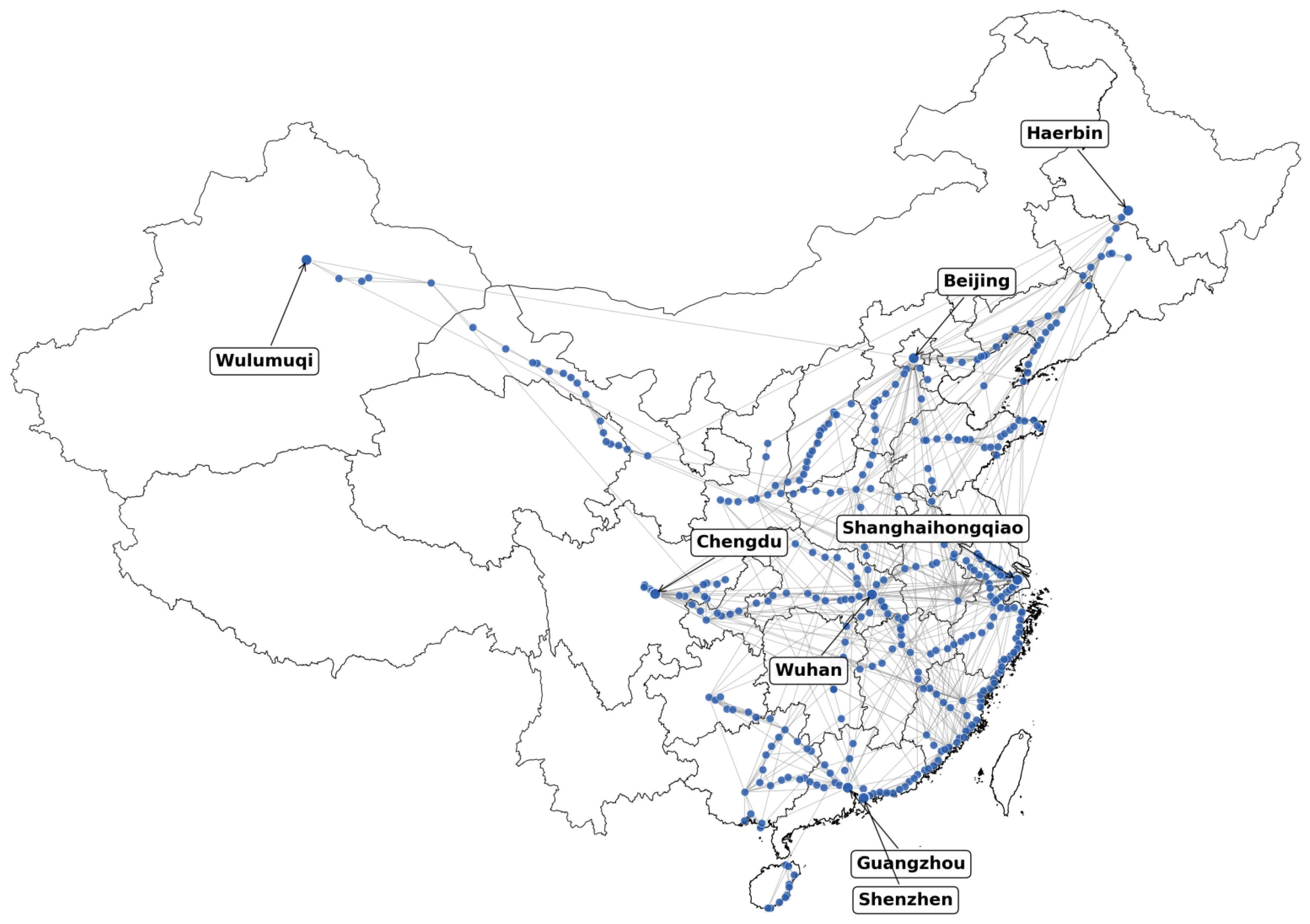
Figure 1. China’s High-Speed Railway network structure.
Bdcc 09 00101 g001
Figure 2. The spatial distributions of key nodes (a) and hub cities (b).
Bdcc 09 00101 g002
Figure 3. Degree distributions of China’s HSR network.
Bdcc 09 00101 g003
Figure 4. Robustness of China’s HSR network.
Bdcc 09 00101 g004
Figure 5. Key node distribution on a map of China.
Bdcc 09 00101 g005
Figure 6. Communities in China’s HSR network.
Bdcc 09 00101 g006
Figure 7. Node distribution by community and type.
Bdcc 09 00101 g007
Figure 8. The node density degrees of communities.
Bdcc 09 00101 g008
Figure 9. Important pathways among communities in China’s HSR network.
Bdcc 09 00101 g009
Figure 10. Distributions of sample communities.
Bdcc 09 00101 g010
Figure 11. Potential links in the HSR network.
Bdcc 09 00101 g011
Table 1. The key characteristics of China’s HSR network.
Number of nodes379Number of edges1096
Max degree35Min degree1
Average clustering coefficient (C)0.5786Average shortest path length (L)4.2145
Random network clustering coefficient ( C Random )0.0104Random network characteristic path length ( L Random )3.5940
Table 2. Top 20 key nodes by degree.
RankNameDegreeRankNameDegree
1Fuzhou3511Wuhan20
2Beijing3312Changchun17
3(SH) Hongqiao3213Guangzhou16
4Hankou3114Chongqing16
5Nanjing3115Nanning16
6Nanchang2516Ningbo16
7Xiamen2317Guilin16
8Hangzhou2318Zhengzhou16
9Chengdu2219Wenzhou16
10Shenyang2120Taiyuan16
Table 3. Efficiency measures of China’s HSR network.
Global Efficiency ( E glob )0.2720Assortativity Coefficient (r)0.1688
Local Efficiency ( E loc )0.6663Network Density (D)0.0153
Table 4. Key nodes by importance score.
RankNameScoreRankNameScore
1Fuzhou6.51688911Wuhan4.5285864
2(SH) Hongqiao6.161404612Changchun3.893515
3Beijing6.09468713Wenzhou3.7896342
4Haikou5.953695314Chongqing3.7215261
5Nanjing5.9108815Ningbo3.6994753
6Nanchang5.14537816Nanning3.6439276
7Xiamen5.067480617Guangzhou3.639298
8Hangzhou4.76842918Suzhou3.611753
9Chengdu4.630962419Taiyuan3.5928736
10Shenyang4.54469720Guilin3.5588112
Disclaimer/Publisher’s Note: The statements, opinions and data contained in all publications are solely those of the individual author(s) and contributor(s) and not of MDPI and/or the editor(s). MDPI and/or the editor(s) disclaim responsibility for any injury to people or property resulting from any ideas, methods, instructions or products referred to in the content.

