Article

Metadata Suffices: Optimizer-Aware Fake Account Detection with Minimal Multimodal Input

1
Department of Computer Engineering, Istanbul Medipol University, 34810 Istanbul, Turkey
2
Department of Electrical and Electronics Engineering, Istanbul Medipol University, 34810 Istanbul, Turkey
3
Department of Computer Science, University of Calgary, 2500 University Drive NW, Calgary, AB T2N 1N4, Canada
4
Department of Health Informatics, University of Southern Denmark, 5230 Odense, Denmark
*
Authors to whom correspondence should be addressed.
Big Data Cogn. Comput. 2025, 9(12), 298; https://doi.org/10.3390/bdcc9120298
Submission received: 28 September 2025 / Revised: 13 November 2025 / Accepted: 15 November 2025 / Published: 21 November 2025

Abstract

Social media platforms are currently confronted with a substantial problem concerning the presence of fake accounts, which pose a threat by spreading harmful content, spam, and misinformation. This study aims to address the problem by differentiating between fake and real X accounts (formerly Twitter). The need to mitigate the negative impact of fake accounts on online communities serves as the driving force for this work, with the goal of developing an effective method for identifying fake accounts and their fraudulent activities, such as posting harmful links, engaging in spamming behaviors, and disrupting online communities. The scope of this work focuses specifically on fake Twitter account detection. A comprehensive approach is taken, leveraging user information and tweets to discern between genuine and fake accounts. Various deep learning architectures are proposed and implemented, utilizing different optimizers and evaluating performance metrics. The models are trained and tested using a collected dataset, augmented to cover diverse real-life scenarios. The results show promising progress in distinguishing between fake and real accounts, revealing that the inclusion of tweet content along with user metadata does not significantly improve the classification of fake accounts. It also highlights the importance of selecting appropriate optimizers. The implications of this study are relevant to social media platforms, users, and researchers. The findings provide insights into combating fake accounts and their fraudulent activities, contributing to the enhancement of online community safety. While the research is specific to Twitter, the methodology and insights gained may be potentially generalizable to other social media platforms.

1. Introduction

Social Media affects all aspects of human lives; the way they think, act, talk, and behave, and what they buy, dress, and eat. It transcends boundaries, connecting diverse global audiences and cultures [1]. Social media usage spans across various demographics and is expected to grow to new users over time. While it has brought numerous benefits and opportunities, it has also raised concerns about privacy, misinformation, addiction, and other psychological impacts [1]. As social media evolves and shapes society, it is crucial to understand its effects and implications. Like any tool, social media can be used for both constructive and harmful purposes, such as sharing useful information, saving people’s time and money, or manipulation and scamming others for personal gains [2].
Like any enterprise striving to flourish and surpass competitors in its industry, social media platforms are constantly experimenting with various algorithms and techniques to determine which content should be prioritized and promoted to attract more users and generate greater profits, while burying and concealing other content. The primary measure for this is the level of engagement a user receives on their content, which can manifest in various forms and names, contingent on the platform. These may include actions such as “like,” “dislike,” “love,” “angry,” “comment,” “share,” “retweet,” “report,” “follow,” and “unfollow,” among others. A prevalent method for gauging a user’s popularity is by tallying their number of followers, as well as the amount of likes or retweets their content receives. Malicious actors can exploit this fact through various ways to reach people, spread their poisons and achieve their goals [3].
In the real world, a person can be easily identified and verified through some unique official documents that are issued only to him and hard to forfeit (ID, driving license, and passport). These documents contain a set of identifiers that cannot be duplicated by any means, such as name, fingerprints, photograph, birth date, and blood type, etc. The situation is much different on social media, where each user is identified by a profile, including some basic information about him, such as his name, photo, and birth date, with no real authority to check and validate this data. To create an account, most of the platforms require only one unique email. So, with no real unified checking authority, it has become a very easy task to forge or fake your identity on social media [4].
The identity of a person on social media can be either real, false, or fake. A real identity, having only one unique account that is created using his information and being used solely and freely by the person himself. In the case of a false identity, a user would use someone else’s (mostly a celebrity, famous figure, or organization) identity and information to create an account and disguise himself as the celebrity. In case of a fake identity, a person would create accounts using invented names and information that may coincide with real persons [5]. Detecting false identities is relatively easier than detecting fake identities. The focus of this study is to capture these fake accounts on Twitter created using some invented identities for various malicious causes such as sharing fake news, misleading web ratings, and spam.

Problem Definition and Motivation

Social media has brought an overwhelming influx of news and information spanning across every corner of the globe. With a diverse range of individuals behind these posts, each driven by their own unique intentions and agendas, it becomes increasingly challenging, and sometimes even impossible, to ensure that every piece of content shared on these platforms is both ethical and reliable. Hence, it is important to have an automated process capable of differentiating fake from real content. This includes identifying accounts that are dedicated to broadcasting false information, known as fake accounts. This study aims to address the significant threat posed by fake accounts on social media, which can propagate various forms of harmful content, spam, and misinformation. Examples of fraudulent activities that fake accounts can engage in include posting harmful links, spamming mass follow/unfollow requests, repeatedly sharing unrelated links and ads, stealing personal information, as well as disrupting online communities by ways of trolling, hate speech, and harassment. The goal of this study is to differentiate between fake and real accounts on X (formerly Twitter) by leveraging user information and tweets.

2. Related Work

Social media researchers and platforms use various methods and techniques to detect fraudulent accounts.  [3] broadly categorized these methods into two types:
  • Techniques that focus on analyzing the traits and relationships of individual accounts (profile-based and graph-based methods);
  • Techniques that aim to detect organized activity by large groups of accounts (e.g.,crowdturfing).
In [4], with an accuracy of 84.5%, the authors have recognized 23 characteristics for categorizing Twitter spammer/non spammer accounts. Ref. [6] utilized a smaller set of 10 features, with less promising results. The work described in [7] employs an SVM to classify fake profiles in a Facebook game. To do so, they extract 13 features for each game user. Instead of using some individual profile-based features, other approaches relied on graph-based features in this classification task [8,9]. The work described in [10] relies on the observation that fake profiles tend to establish connections predominantly with other fake profiles rather than legitimate ones. As a result, a distinct separation exists between the subgraphs comprising fake and non-fake accounts in the graph. While on the other hand, the authors of [11] claim the opposite; fake accounts do not exclusively associate with other fake accounts, and present a new detection methodology centered around the analysis of features exhibited by victims’ accounts. Another approach used by researchers in this context is the study of the change of user behavior, which may happen in cases like the exploitation of a legitimate account that temporally acts maliciously. For example, anomalous behavior can be detected by monitoring some features such as timing and the origin of messages, language, and message topic, URLs, use of direct interaction, geographical proximity [12].
In the approaches trying to capture coordinated activities of large groups of accounts, the black market and fake accounts online sellers play a major role, with a large segment of customers that may vary from celebrities, politicians, to cyber criminals. Ref. [13] describes the characteristics of the Twitter follower market, arguing that there are two major types of accounts that may follow a customer: either fake accounts or compromised accounts. The work described in [14] shows the danger of crowdturfing, in which workers are paid to express a false digital impression. They start first by describing the operational structure of such systems and how it can be used to build a whole fake campaign. The authors build a benign campaign on their own to show how easy and dangerous the process can be. Ref. [15] conducted research on the feasibility of using machine learning techniques to identify crowdturfing campaigns, as well as the resilience of these methods against potential evasive tactics employed by malicious actors. According to their findings, traditional machine learning methods can effectively detect crowdturfing workers with an accuracy rate of 95–99%. However, these detection mechanisms can be circumvented if the workers modify their behavior.
Most of the works mentioned earlier require historical data as they heavily depend on extensive content or behavior. Therefore, they encounter a significant drawback of time delay, whereby the fake user may have already executed numerous malicious activities before being identified and eliminated. To address this concern, Ref. [16] developed a system to detect fake accounts directly after registration. Their approach involves analyzing both user behavior and content to identify any suspicious patterns or activities. The methodology includes the extraction of synchronization-based and anomaly-based features. The authors in [17,18] present a method for detecting social spammers by using social honeypots and machine learning. Initially, multiple honeypots were deployed to lure social spammers, and then an ML model is trained using features derived from the gathered data of these honeypots. The work described in [19] examines various features used in detecting Twitter accounts, creating a dataset comprising both human and fake follower accounts. They then evaluate several machine learning classifiers using this dataset and introduce their own classifier. The authors found that features based on the friends and followers of the account being investigated yielded the best results among all the analyzed features .
Another approach to tackling the issue of detecting spam on Twitter is to concentrate on the tweet itself instead of user information. Ref. [20] proposed a method in which features were extracted from the content of the tweet, such as the presence of particular keywords, URLs, and hashtags, as well as tweet structure (e.g., length, capitalization, and punctuation usage). Additionally, the temporal pattern of tweets was analyzed as a feature, with the authors discovering that spam tweets are frequently posted in bursts, while genuine tweets are more evenly distributed over time. The authors utilized machine learning algorithms to discover patterns in these features and differentiate between spam and genuine tweets. In [21], the authors suggest a method for performing sentiment analysis on Twitter data by utilizing the Naïve Bayes classifier. Using a dataset of 10,000 tweets collected from Twitter and manually categorized as positive, negative, or neutral. Various features are extracted from the preprocessed data, such as specific words or phrases, and used to train the Naïve Bayes classifier. The results of the study indicated an accuracy of 80.5% for sentiment classification of Twitter data using this approach. To tackle evasion techniques used by spammers, some works try to use more robust features; Refs. [22,23] propose some hybrid frameworks; Ref. [22] exploits users’metadata, graph-based and text-based features, and found that Random Forest gives the best performance. Similarly, Ref. [23] use four sets of features in theirclassification, including account-based, text-based, graph-based, and automation-based features. Other approaches rely on DL techniques, e.g., Ref. [24] uses Word2Vec deep learning technique to preprocess their dataset and then assign a multi-dimensional vector to a tweet. Ref. [25] developed two classifiers: a text-based classifier that only considers user tweet text, and a combined classifier that uses CNNs to identify relevant features from high-dimensional vector representations of tweet text and applies Dense layers on users’ metadata information. Overall, the combined model shows better results.
Recent works utilize more complex architectures and hybrid approaches to enhance fake account detection on platforms like X. For instance, Ref. [26] introduced BotMoE, a mixture-of-experts model using community-aware features for Twitter bots, achieving high precision via modal-specific experts. Ref. [27] developed Twibot-22, a graph benchmark integrating profiles, text, and networks for scalable detection. Ref. [28] proposed BotArtist, a semi-automatic pipeline on profile features across nine datasets, outperforming 35 baselines (F1: 83.19%) with low API costs. Recent multimodal works align with our hybrid approach. For instance, the work described in [29] presented TMTM, combining RoBERTa text embeddings, user features (46 attributes), and relational graph neural networks (R-GCN) on Twibot-22, improving F1 by 5.48% via enriched features, highlighting text’s marginal gains, echoing our findings. The work described in [30] used CNNs on Twitter profile images/metadata, reaching 92% accuracy for bots/cyborgs, but noted real-world drops due to dynamic behaviors. Ref. [31] offered an unsupervised Sliding Histogram for coordinated fake-follower campaigns, detecting anomalies in follow patterns without labels, scalable for large-scale analysis. Ref. [32] explored human-bot detection psychology, finding feature overlaps challenge simple classifiers. Globally, the work described in [33] compared bot/human traits, revealing 20% bot chatter with distinct patterns. Ref. [34] characterized spam prevalence, linking 22% of news links to top bots.
Our work will build on these as a baseline, Simple Dense and LSTM hybrids for reproducibility, focusing on optimizer impacts amid evolving platforms [34]. Unlike transformer-heavy models [26,29], we prioritize scalability over complexity.
To contextualize our approach, Table 1 summarizes and compares key characteristics of some representative recent fake account detection works, including methods, datasets, and reported performance metrics.
Shortcomings of the related work may be enumerated as follows:
  • Narrow Focus: Many of the works discussed in the literature review target specific types of fake users or spammers within a narrow domain. This limited focus may not capture the full range of fraudulent activities on social media platforms.
  • Dependency on Historical Data: Several approaches heavily rely on historical data, either content-based or behavior-based, which poses a significant drawback of time delay. By  the time the fake user is identified and eliminated, they may have already executed numerous malicious activities.
  • Limited Robustness: Some of the detection methods can be evaded or circumvented if the fraudulent actors modify their behavior or tactics. This undermines the robustness of the detection mechanisms and raises concerns about their effectiveness in real-world scenarios.
  • Costly Implementation: Certain approaches, such as graph-based methods, can be computationally expensive and require extensive resources for implementation. This can limit their applicability in large-scale settings.
  • Lack of Comprehensive Features: Some studies focus on a limited set of features, either profile-based or tweet-based, without considering a comprehensive range of indicators. This may result in incomplete detection and overlook certain patterns or characteristics of fake accounts.
  • Limited Generalizability: The performance of some detection methods may be limited to specific datasets or contexts, making it challenging to generalize their effectiveness to different social media platforms or scenarios.
  • Lack of Comparative Analysis: Some works present results without a comparative analysis of different methods, making it difficult to assess the relative performance and strengths of each approach.
  • Incomplete Coverage of Spam Detection: While some studies concentrate on fake user detection, there is a lack of comprehensive coverage of spam detection in the context of Twitter, with limited focus on analyzing tweet content and sentiment analysis.
Overall, the shortcomings of the related work include limited scope, dependency on historical data, potential evasion by fraudulent actors, costly implementation, lack of comprehensive features, limited generalizability, lack of comparative analysis, and incomplete coverage of spam detection. Addressing these limitations would contribute to more effective and robust methods for detecting fraudulent accounts and spam on social media platforms.

3. Objectives and Contributions

The objectives and contributions of this work can be concisely summarized in the following key points:
  • The main objective of this work is to identify fake X(Twitter) accounts using user metadata, such as followers and following numbers, and the tweets posted over time.
  • Combining Numeric and Text Data: The proposed approach combines both numeric and text data to detect fake Twitter accounts. This integration of different types of data provides a more comprehensive analysis.
  • Two-Branch Deep Learning Model: To achieve this objective, a two-branch deep learning model is implemented. One branch utilizes dense layers, while the other branch employs LSTM (Long Short-Term Memory) layers. This architecture permits the model to discover relevant patterns and features from the mixed data.
  • Evaluation of Traditional and Simpler Models: We initially explore some traditional and simpler models to assess their performance on the given type of data. This step helps establish a baseline and provides a comparison point for the effectiveness of the proposed approach.
  • Data Generation and Augmentation: In order to train and evaluate the two-branch DL model, two real-world Twitter datasets are collected, merged, and augmented. This step ensures a diverse and representative dataset for model training and testing.
  • Model Comparison: To ensure a comprehensive comparison, all implemented and trained models underwent evaluation and testing on unseen data using various metrics and indicators. These metrics include model accuracy and loss, confusion matrix(CM), precision, recall, F1 and F2 scores, and Matthews Correlation Coefficient (MCC). By considering these metrics, a thorough assessment of the models’ performance can be obtained.
In summary, this study contributes by using a novel approach that combines numeric and text data for identifying fake Twitter accounts. It also explores the effectiveness of a two-branch deep learning model in handling mixed data and achieving moderate success in detecting fake accounts. The utilization of real-world Twitter datasets and the evaluation of traditional models provide valuable insights into the challenges and potential solutions in this domain.

4. Methodology

4.1. Components of the Developed Methodology

The methodology developed for this study involves trialing various models, as illustrated in Figure 1, which shows all the components of the methodology. The process consists of several stages, including analysis, data collection, data preprocessing, data augmentation, model implementation and training, model evaluation, and result comparison. During analysis, similar works and models are observed, and a few of them are selected for implementation and testing. Labelled data is then collected from different resources and organized during data collection. Data preprocessing involves performing all the necessary operations to format and shape the data for use in the model, including dividing the dataset into test and train sets. Data augmentation is used to generate new data points that do not exist in the original dataset and can simulate real-world data from various scenarios. The model implementation and training stage involves setting up the environment, importing the necessary libraries and frameworks, and defining the model. Hyperparameters are selected, and the training process is initiated using the training set. Model evaluation is then conducted to assess the model’s performance on data that it has not been trained on before (the test set). Finally, if the model fits, achieved results and scores are recorded and compared with other implementations.

4.2. Data Sets

While two public datasets serve as the foundation for this study, all models were trained and evaluated exclusively on a derived, balanced, and augmented dataset (Table 2), constructed by merging, cleaning, and synthetically expanding samples from these sources as detailed in Section 4.2.1Section 4.2.3.
Data utilized in this study were gathered from multiple sources, including some that were augmented based on the obtained ones.
This work utilized two Main types of datasets for model training:
  • unbalanced dataset: consists of 2,614,000 real users labelled as 0 and 187,329 fake users labelled as 1. This dataset was obtained before any balancing process was applied. While it is generally not advisable to use such a dataset with a significant disparity in the number of instances per class, as it may result in subpar performance, it can be utilized in certain situations to study the influence of utilizing both balanced and unbalanced datasets on the same model.
  • A balanced dataset (used in this work): containing 374,658 records, with 187,329 instances in each class. This dataset was divided into train and test sets of 299,726 and 74,932 records, respectively. Following that, the dataset was augmented into a larger one with a final balanced dataset of 474,658 records divided into 369,726 training instances, and 104,932 test records. Table 2 demonstrates the distribution of the final utilized dataset in this study.

4.2.1. Data Collection

To encompass a wide range of subjects and locations, multiple sources were utilized in compiling these datasets. The following is a selection of the datasets incorporated, along with their corresponding contexts.
Dataset 1 Fame for Sale: Efficient Detection of Fake Twitter Followers [19]
A dataset of both verified humans and Fake followers accounts, consisting of 5 subfolders, each of which contains 4 CSV files: ‘followers.csv’, ‘tweets.csv’, ‘friends.csv’, and ‘users.csv’.
This dataset is available at: “http://mib.projects.iit.cnr.it/dataset.html, accessed on 11 November 2025”. TFP and E13 represent real human accounts, while the other three datasets, TWT, INT, and FSF, represent fake followers. Table 3 shows some statistics about this dataset.
  • The Fake Project(TFP)
    TheFakeProject is a research initiative started in 2012 by IIT-CNR researchers, who created a Twitter account @TheFakeProject and collected public information using Twitter APIs. They obtained 616,193 tweets and 971,649 relationships. resulting in 469 “certified humans.” The dataset is called TFP.
  • Elezioni2013 dataset(E13)
    The #elezioni2013 dataset was created for a sociological study on the changes in Italian politics from 2013 to 2015. A total of 84,033 unique Twitter accounts that utilized the hashtag were identified, and accounts belonging to politicians, parties, journalists, and bloggers were discarded, leaving about 40k accounts classified as citizens. A sample of 1488 accounts was manually verified by analyzing profile pictures, biographies, and  timelines, and 1481 accounts were included in the dataset.
  • Intertwitter dataset (INT)
    In April 2013, 1337 fake accounts were bought and crawled from “http://intertwitter.com, accessed on 11 November 2025”, to build the intertwitter dataset labelled as INT.
  • Fastfollowerz dataset (FSF)
    In April 2013, 1169 fake accounts were bought and crawled from “http://fastfollowerz.com, accessed on 11 November 2025”, to build the fastfollowerz dataset labelled FSF.
  • Twittertechnology dataset (TWT)
    In April 2013, 1000 fake accounts were bought from “https://web.archive.org/web/20130821031300/, accessed on 11 November 2025”. Almost instantly, 155 of them were suspended, and the remaining 845 were crawled in order to build the twittertechnology dataset labelled as TWT.
As mentioned, each subfolder contains four CSV files, and each dataset contains the same file architecture and attributes. For instance; in Twittertechnology dataset (TWT), the attributes in each file are as follows:
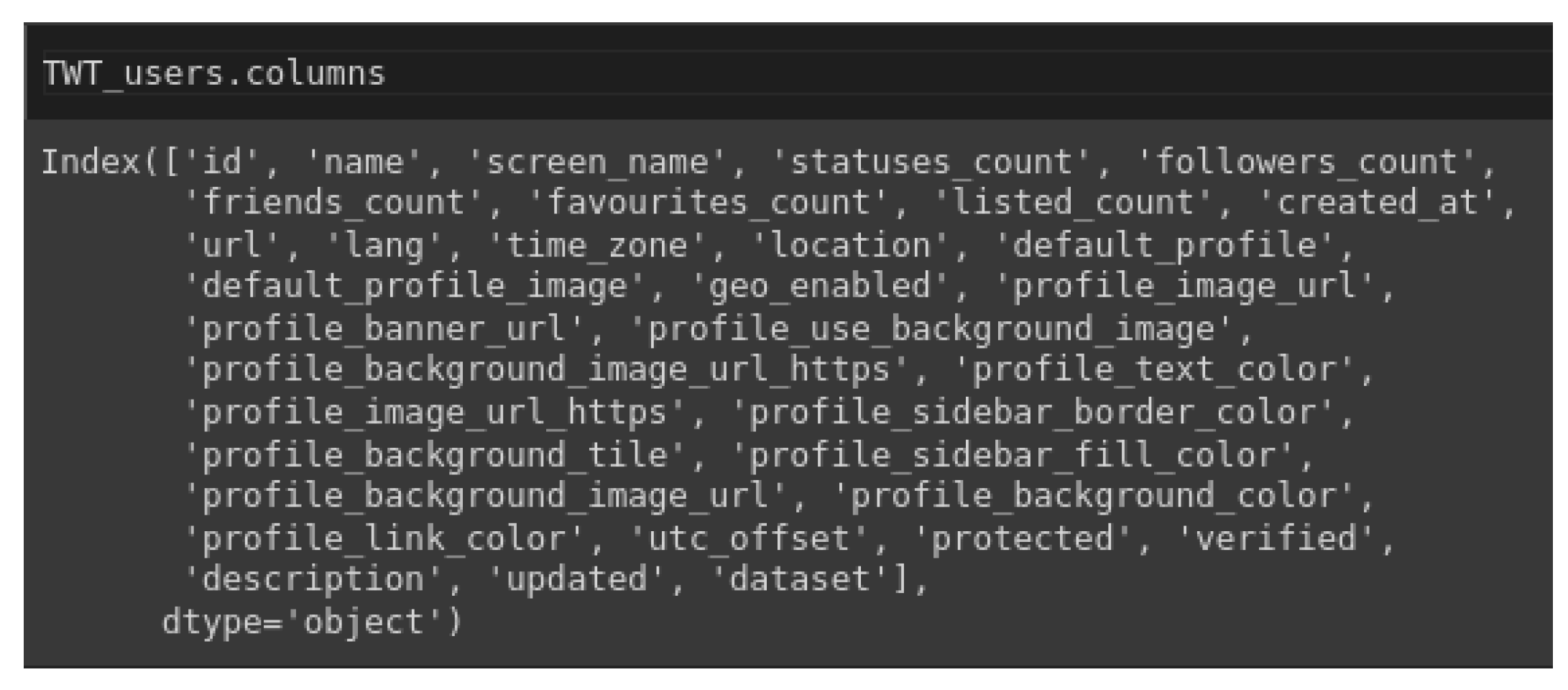
  • users.csv: contains 34 attributes listed in Figure 2
  • followers.csv: contains two attributes, which are source id and target id, as shown in Figure 3
  • tweets.csv: contains 19 attributes that are listed in Figure 4
  • friends.csv: contains 2 attributes as shown in Figure 5 which are source id and target id
dataset2: Social Honeypot Dataset [18]
A dataset of social honeypots, gathered from Twitter over a period of seven months and used in a study called “Seven Months with the Devils: A Long-Term Study of Content Polluters on Twitter” [18]. The dataset includes 22,223 content polluters and their followers numbers, 2,353,473 tweets, and 19,276 legitimate users and their number of followers, along with 3,259,693 tweets. As mentioned in the dataset Readme File, it consists of six text files:
  • content polluters.txt
  • content polluters followings.txt
  • content polluters tweets.txt
  • legitimate users.txt
  • legitimate users followings.txt
  • legitimate users tweets.txt
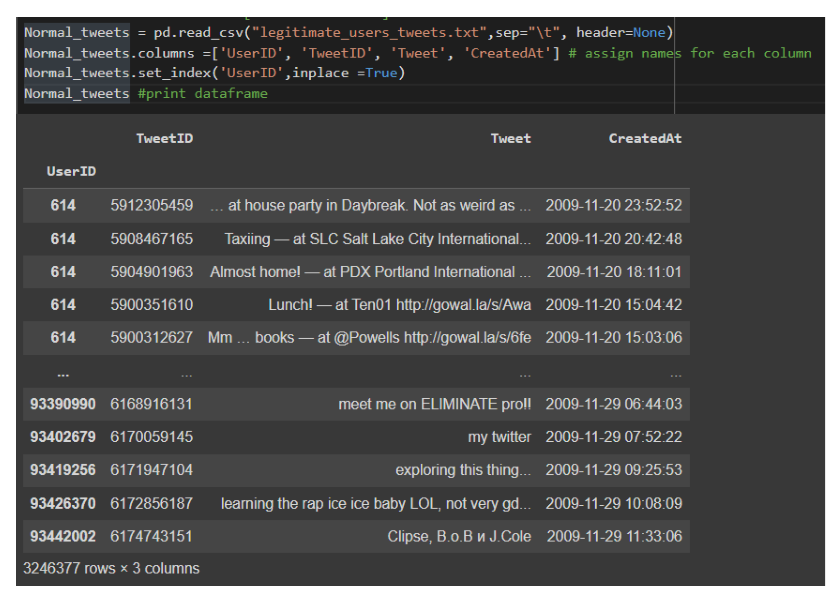
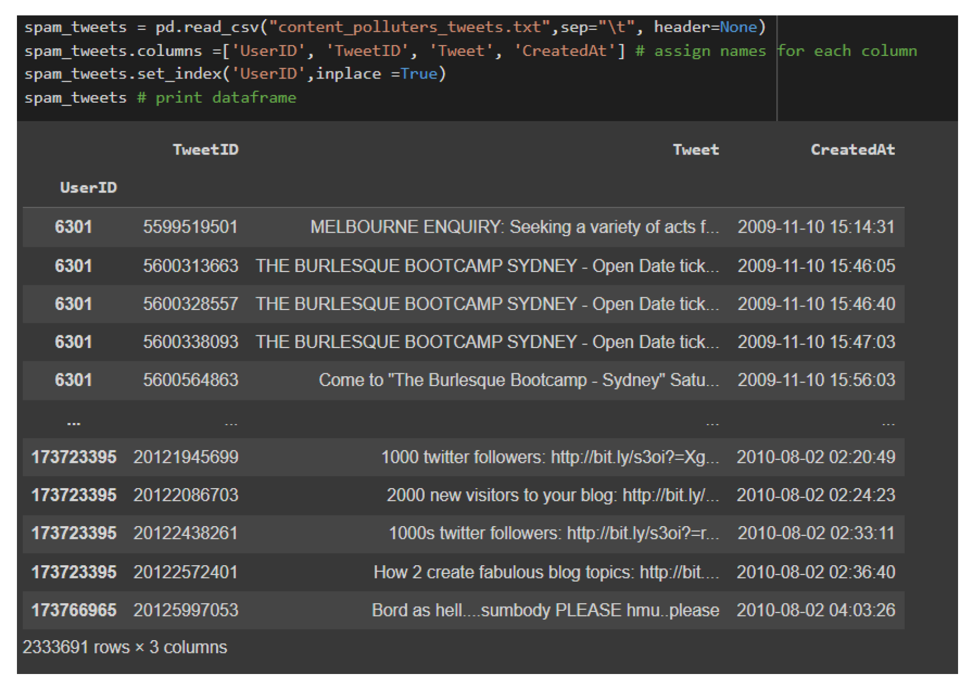
As the dataset’s features differ from the first one, only the tweets from this dataset will be utilized. “legitimate users tweets.txt” and “content polluters tweets.txt” are the two essential files for the augmentation process, as they contain the tweets to be employed in the process. Figure 6 and Figure 7 are samples of both files after being imported into python notebook.

4.2.2. Data Preprocessing

As various models were utilized and evaluated, the approach to data preparation differed. For instance, certain models solely required an 8-dimensional vector of user metadata as input, whereas another model necessitated a 308-dimensional vector combining tweet and text representations. As a result, two distinct formats were created.
Format 1: user meta data
For models that require only some user information (metadata), and based on the feature analysis made by [19], seven features were selected, and one extra feature was extracted from them. These features include the following: statuses count, followers count, friends count, favorites count, listed count, URL, and time zone. The last feature that was extracted from them is “user score”. Equation (1) shows how user score “score” is calculated for each record in the dataset
s c o r e = f 1 [ i ] f 1 · max f 2 [ i ] f 2 · max + f 3 [ i ] f 3 · max .
Such that:
  • score: user score
  • i: record number inside the Pandas DataFrame
  • max: maximum value of a feature in the whole DataFrame
  • f1: followers count
  • f2: friends count
  • f3: number of tweets
Note that Format 1 is essentially a subset of Format 2 described in the following section. Therefore, once the data is formatted as Format 2, it is sliced to extract only the first eight pieces of user data and the corresponding record label, while eliminating any duplicates.
Format 2: user meta data + user tweet
For models that require both user information and tweet text, the same eight previous features are utilized, along with an added vector representation for each tweet. To vectorize the tweets, a pre-trained NLP library (Spacy [41]) is utilized to obtain a 300-dimensional vector representation for each tweet. Note that the dataset was prepared in batches, owing to constraints on memory and disk space.
The data preprocessing pipeline begins by loading the raw users.csv and tweets.csv files from both datasets, and importing all necessary libraries. A new DataFrame is initialized to store the processed records, containing the following user metadata fields (from users.csv): statuses_count, followers_count, friends_count, favourites_count, listed_count, URL, time_zone and dataset, and a derived user_score(computed via Equation (1)). Using the user ID, a loop is executed to search for matches in the user ID column in Tweets.csv. Each time a match is found, the previous nine values of the record are duplicated into a new record, followed by the tweet, which is vectorized into a 300-dimensional embedding using the pre-trained SpaCy English language model. Categorical features (URL and time_zone) are mapped to numeric values, and all numeric columns are normalized to the [0, 1] range using min-max scaling. Missing values are removed by dropping empty rows, and any remaining NaN entries are imputed as zero. Duplicate records are eliminated to ensure sample uniqueness. Finally, labels are assigned such that real accounts are marked as 0 and fake accounts as 1, and the dataset is balanced via random undersampling to contain equal numbers of both classes before being split into training (80%) and test (20%) sets. The full preprocessing workflow is summarized in Algorithm 1.
Algorithm 1 Data Preprocessing Pipeline
Require: Raw users.csv, tweets.csv from Cresci [19] and Social Honeypot [18]
Ensure: Balanced, normalized dataset with labels
  1:
Load users.csv and tweets.csv
  2:
Merge on user_id; keep first tweet per user
  3:
Map categorical features (URL, time_zone) to numeric values
  4:
Compute user_score using Equation (1):
     score = followers max ( followers ) friends max ( friends ) + statuses max ( statuses )
  5:
Vectorize tweet text using SpaCy 300-d pre-trained model
  6:
Normalize all numeric features to [ 0 , 1 ]
  7:
Remove rows with missing values
  8:
Deduplicate by user_id
  9:
Assign label: 0 = real, 1 = fake
10:
Balance classes via random undersampling
11:
Split into train (80%) and test (20%) sets
12:
return Preprocessed dataset

4.2.3. Data Augmentation

To develop a comprehensive model capable of detecting diverse types of spammers and fraudulent accounts, it is imperative to train it on a broad spectrum of data that encompasses various real-world contexts and scenarios. This approach contrasts with datasets such as E13, which was tailored exclusively for political contexts. To accomplish this, a new dataset was constructed to simulate real-world variability by incorporating not only the original dataset [19] but also randomly selected tweets from the Social Honeypot Dataset [20]. For each class, we employed a baseline random sampling within observed minimum and maximum ranges for non-text features [42], ensuring reproducibility without advanced simulation, a practice commonly observed in profile-based studies [30]. The augmentation process commenced with an analysis of each class in the dataset, resulting in an augmented dataset comprising 100,000 records (50,000 for each label). Specifically, for each label, the minimum and maximum values for every feature were determined, followed by the generation of random values within these bounds; for binary features restricted to 0 or 1, random selection between these values was applied. Regarding text vector representation, the identical transformation process to produce 300-dimensional vectors was utilized on selected tweets from dataset 2 [18].
While data augmentation enhanced dataset size and diversity, we acknowledge the potential risk of overfitting or data leakage due to the mixing of original and augmented samples during the train/validation split. Although a formal control using only unaugmented data was not conducted due to resource constraints, preliminary trials with simpler architectures suggested improved generalization with augmentation. To mitigate risks, we monitored convergence behavior closely and applied strict early stopping on validation loss.

4.2.4. Ethical Considerations

All data used in this study were obtained from publicly available and anonymized datasets -namely, the Fame for Sale dataset [19] and the Social Honeypot dataset [18], which were originally collected and shared by researchers for academic purposes. These datasets contain no personally identifiable information (PII) beyond what is publicly visible on Twitter/X user profiles (e.g., follower count, tweet text, time zone), and all user identifiers have been anonymized or removed in the published versions.
This research adheres to ethical guidelines for the use of public social media data. It does not attempt to re-identify users, does not collect new data from live platforms, and is conducted solely for non-commercial, academic purposes aimed at improving online safety. No human subjects were involved, and no institutional ethics approval was required under applicable regulations for the use of fully anonymized, publicly archived data.

4.3. Details of the Proposed Method

Different models and implementations were experimented with and adjusted. The approach was influenced by the methodology described in reference [25]. The objective was to determine which approach would yield superior results in the classification task: utilizing only user metadata or incorporating both metadata and the text of user tweets. To accomplish this, the dataset was gathered and preprocessed. Next, models inspired by relevant prior research were developed and trained on the dataset. Finally, the performance of the models was compared and evaluated based on accuracy and confusion matrix metrics. 2 main types of architectures were used:

4.3.1. One Branched Models

These models follow a single-branch architecture where all the data undergoes sequential layer processing. Such models can perform classification tasks by taking inputs such as user information or tweet text. In this study, only user data was utilized in the one-branch models.

4.3.2. Two Branched Models

This refers to models that employ two parallel branches of layers, with each branch receiving only a specific segment of data per record. One branch is responsible for processing user metadata, while the other processes the user’s tweet text representation. Before the output layer, these two branches are merged together. In Section 5, every implemented model architecture will be showcased in detail, along with various applied variations and their training process. Following that, Section 6 will present the results obtained for each of them.

5. Train and Test Plan

Data preprocessing was performed on a high-memory virtual machine (96 GB RAM, 24-core Intel Xeon E5-2699 v4 @ 2.20 GHz), while all model training and evaluation were conducted using Google Colab notebooks with GPU/TPU support [43]. This environment provides pre-installed deep learning libraries (TensorFlow, Keras, PyTorch, Pandas, NumPy) and can be integrated with Weights and Biases (WandB) for experiment tracking [44].
A total of seven model architectures were implemented: four one-branch models (F-1 to F-4) using only user metadata, and three two-branch models (2B1 to 2B3) combining metadata with tweet embeddings. Each model was trained with four optimizers: Stochastic Gradient Descent (SGD) [45], RMSprop [46], Adam [47], and Adadelta [48]. Additionally, two variants per architecture used SGD with a learning rate reducer (ReduceLROnPlateau, factor = 0.1, patience = 5 on validation loss) [49].
All models were trained for up to 200 epochs with a batch size of 64 and an initial learning rate of 0.015 (or 0.001 for learning rate reducer variants). Early stopping (patience = 7 epochs on validation loss) [50] was applied universally to prevent overfitting. Hyperparameters were initialized based on values commonly used in prior social media classification studies and refined through iterative validation to ensure stable convergence under resource-constrained settings.
Hyperparameter configurations were evaluated through independent training runs for each optimizer and learning rate setting, with model selection guided by early-stopped validation performance and final comparison on the held-out test set. All experiments were tracked using Weights and Biases (WandB), ensuring full traceability of configurations, metrics, and training dynamics across all trials. The complete logs, including loss curves, confusion matrices, and epoch-level metrics for all models, are archived and accessible through the Python notebook and this https://drive.google.com/drive/folders/1-AaK8v68WeYvw8KqpOd1TMINqLS3fCIT, accessed on 11 November 2025.
The naming convention follows:
  • One-branch: F-number-optimizer (e.g., F1-SGD)
  • Two-branch: 2Bnumber-optimizer (e.g., 2B1-Adam)
  • With reducer: …-SGD-lr (0.015)
Performance was evaluated on the test set using a comprehensive set of metrics: accuracy, loss, AUC, precision, recall, specificity, F1/F2 scores, and Matthews Correlation Coefficient (MCC) [51,52].

5.1. Models

This section details the seven deep learning architectures evaluated in this study, categorized into one-branch (F-1 to F-4) and two-branch (2B1 to 2B3) models. Each model is described with its structure, layer configuration, and design rationale. For full architectural transparency, the complete Keras model summary -including layer types, output shapes, and parameter counts for each variant is provided in Appendix C.

5.1.1. F-1 Model

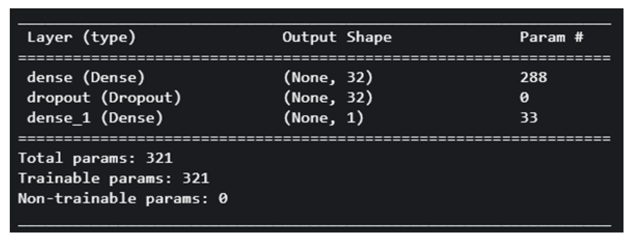
The implemented model described here is the simplest one in this work, comprising only two Dense layers and Dropout. Dense layers, also known as fully connected layers, connect every neuron to all neurons in the previous and subsequent layers, allowing for the learning of non-linear relationships in data [53,54]. Dropout is a technique that randomly selects and deactivates nodes in the network during each training iteration. The selected nodes’ outputs are set to zero, which helps prevent overfitting and promotes a more robust and generalized model [55]. The F-1 model has a total of 321 trainable parameters. Figure 8 demonstrate the architecture of the model.

5.1.2. F-2 Model

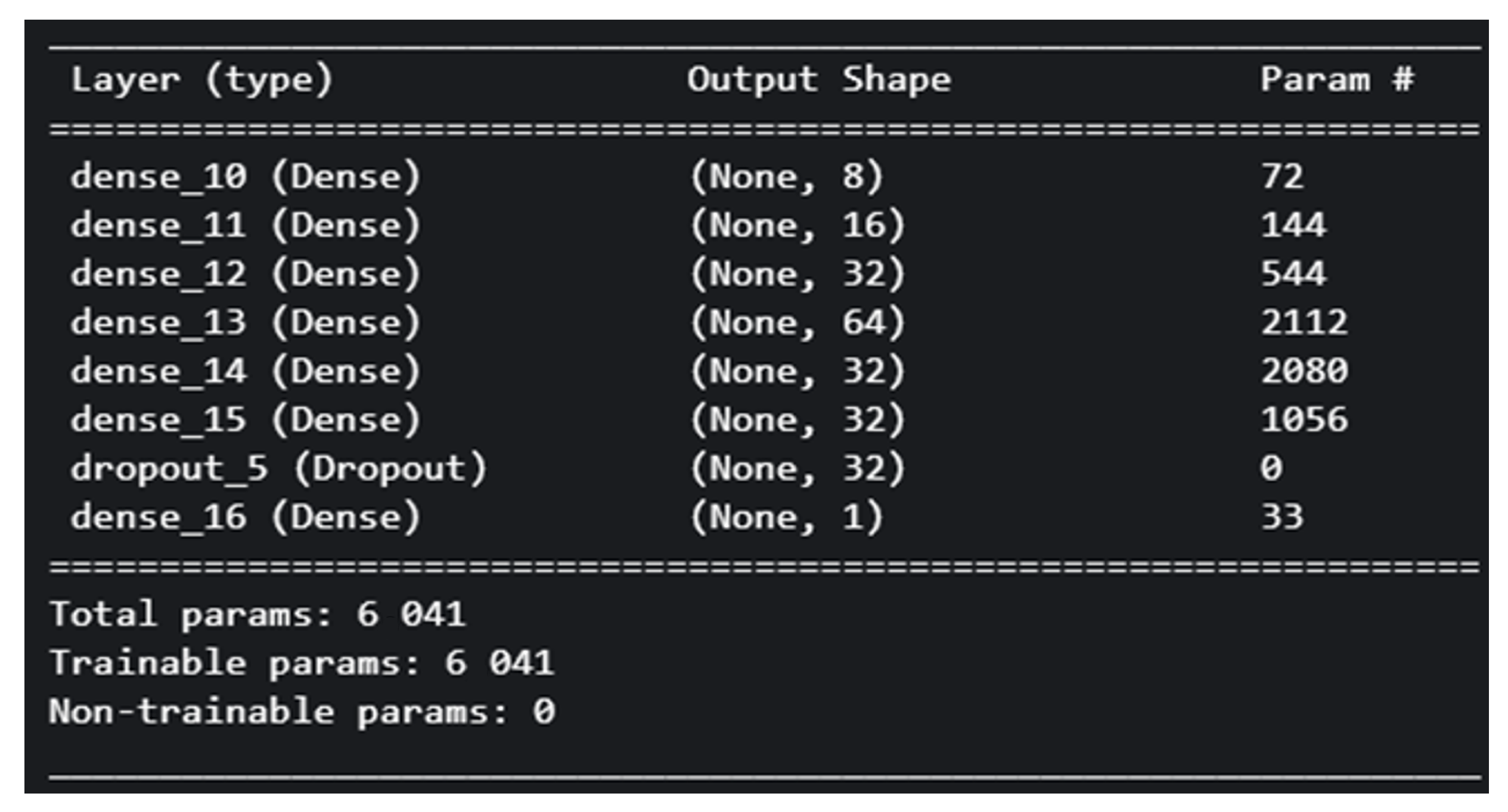
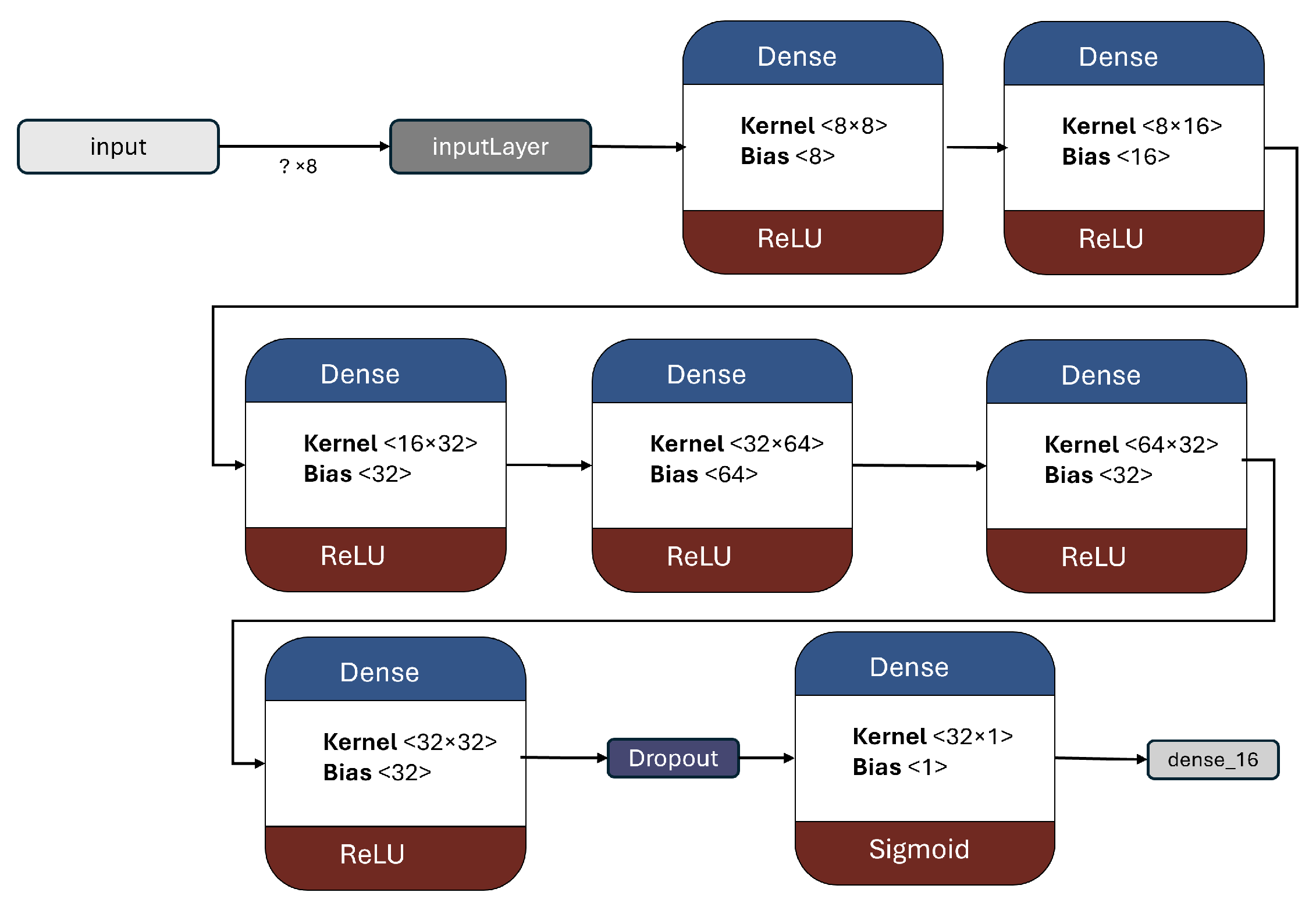
This model is slightly more complex, featuring 7 Dense layers with a greater number of nodes. Having 6041 trainable parameters. Figure 9 showcase the architecture of the model and provide a summary of its key components.

5.1.3. F-3 Model

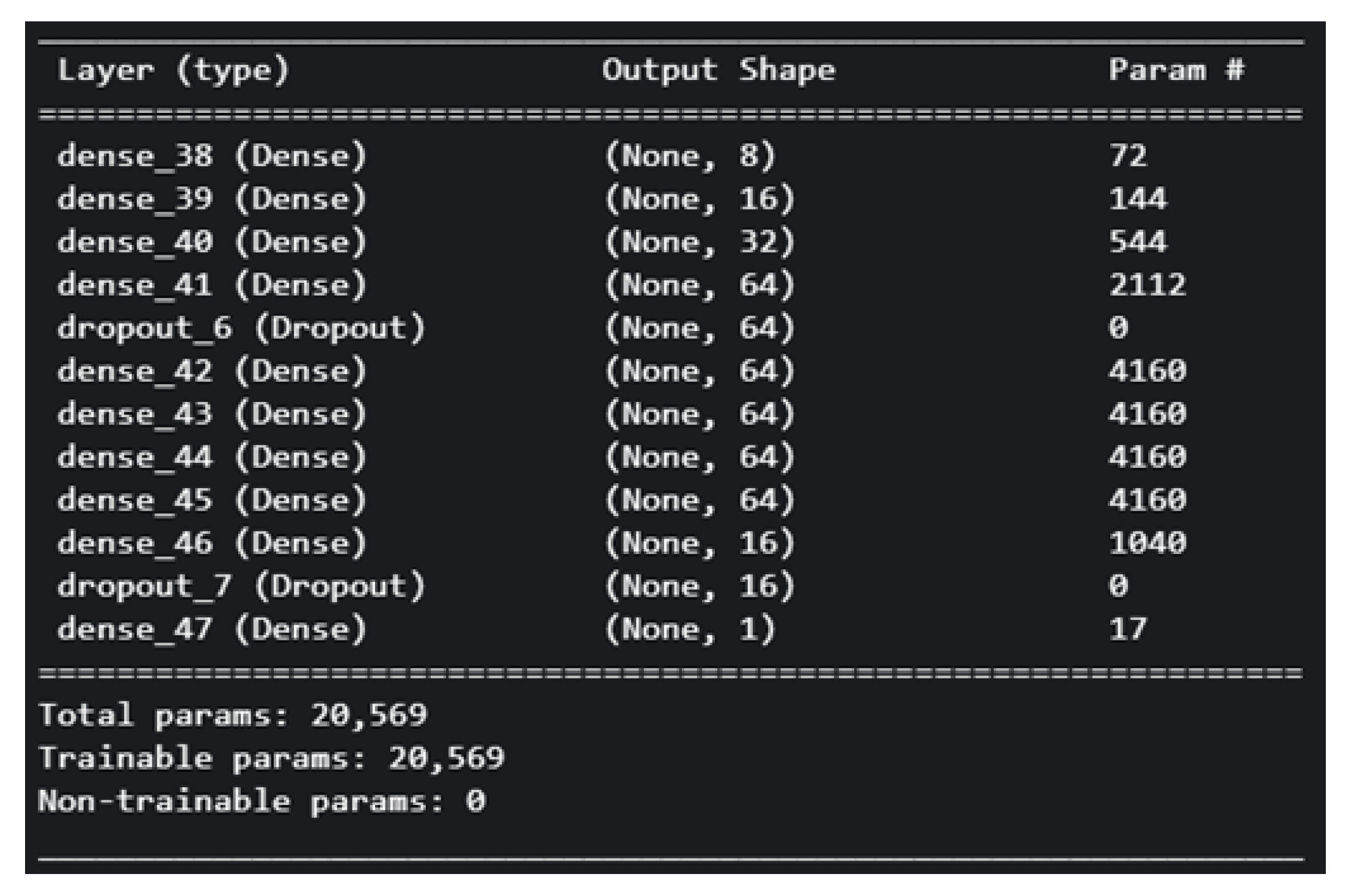
With approximately 3.5 times the number of parameters as F-2, this model boasts a total of 20,569 trainable parameters. Additional layers were incorporated, and the dropout rate was slightly reduced. Figure 10 visually represent the architecture of the model.

5.1.4. F-4 Model

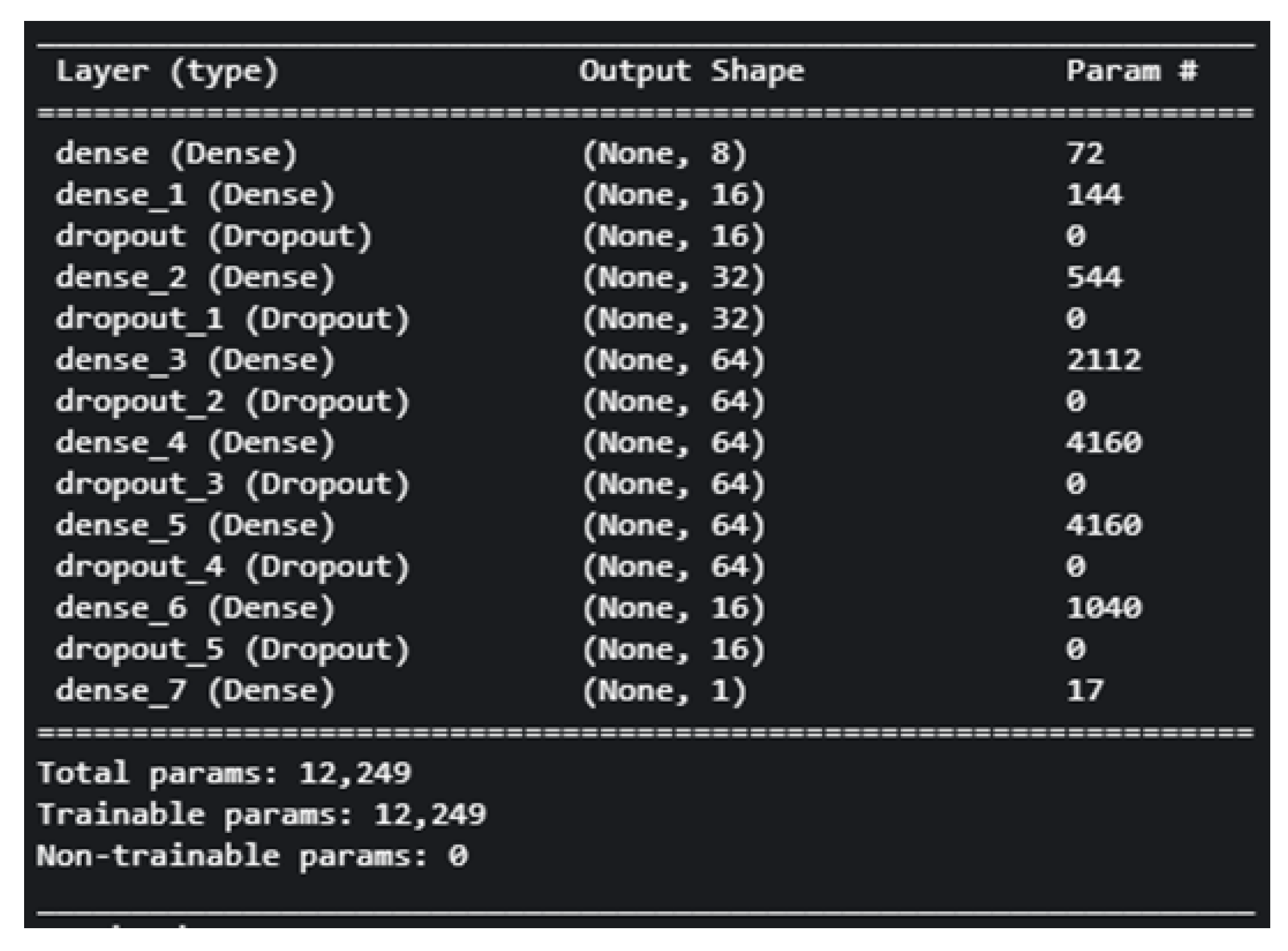
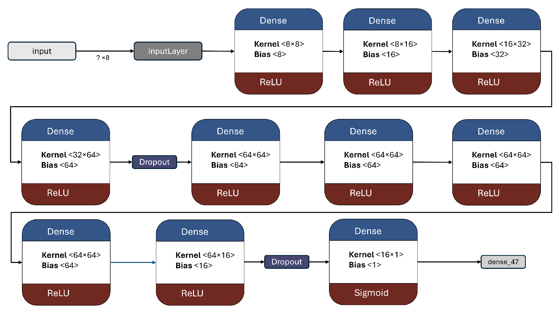
In order to enhance the stability of loss and potentially improve performance, this model introduced additional dropout layers. This approach aimed to assess whether a reduced number of parameters could still yield favorable outcomes. By incorporating more dropout layers, the model aimed to mitigate overfitting and promote generalization. Figure 11 demonstrate the model architecture and characteristics.

5.1.5. 2B1 Model

This model represents a significant advancement in this work, as it incorporates both user metadata and tweet content in a two-branched architecture. The utilization of LSTM in this model allows for the analysis of contextual relationships within the textual representation of tweets. LSTM has demonstrated its effectiveness in various applications, making it a suitable choice for this task.
During the experimentation process, different types of layers were tested on the tweet representation. However, their performance was either negligible or significantly poorer compared to LSTM. As a result, they were not deemed noteworthy for inclusion in this work. The focus remained on leveraging the capabilities of LSTM to extract meaningful information from the tweet text, thereby enhancing the overall performance of the model. While newer architectures like transformers and GNNs achieve high performance, they require substantial computational resources, complex infrastructure, and often external APIs for graph construction, making them impractical for lightweight, real-time deployment. In contrast, LSTM-based models offer a compelling balance; as they can effectively capture sequential text patterns with minimal overhead, enabling efficient training and deployment [26,29,56].
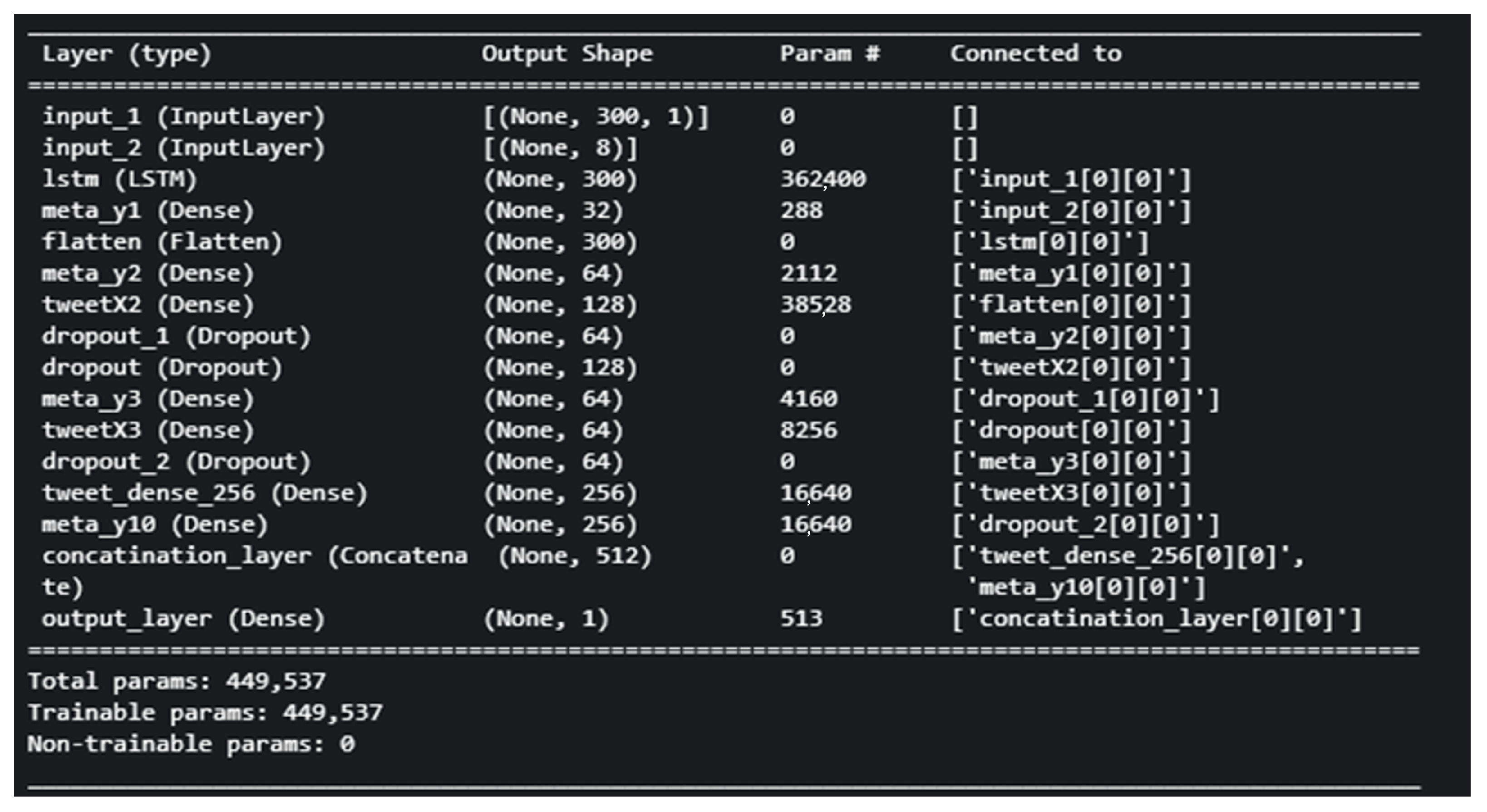
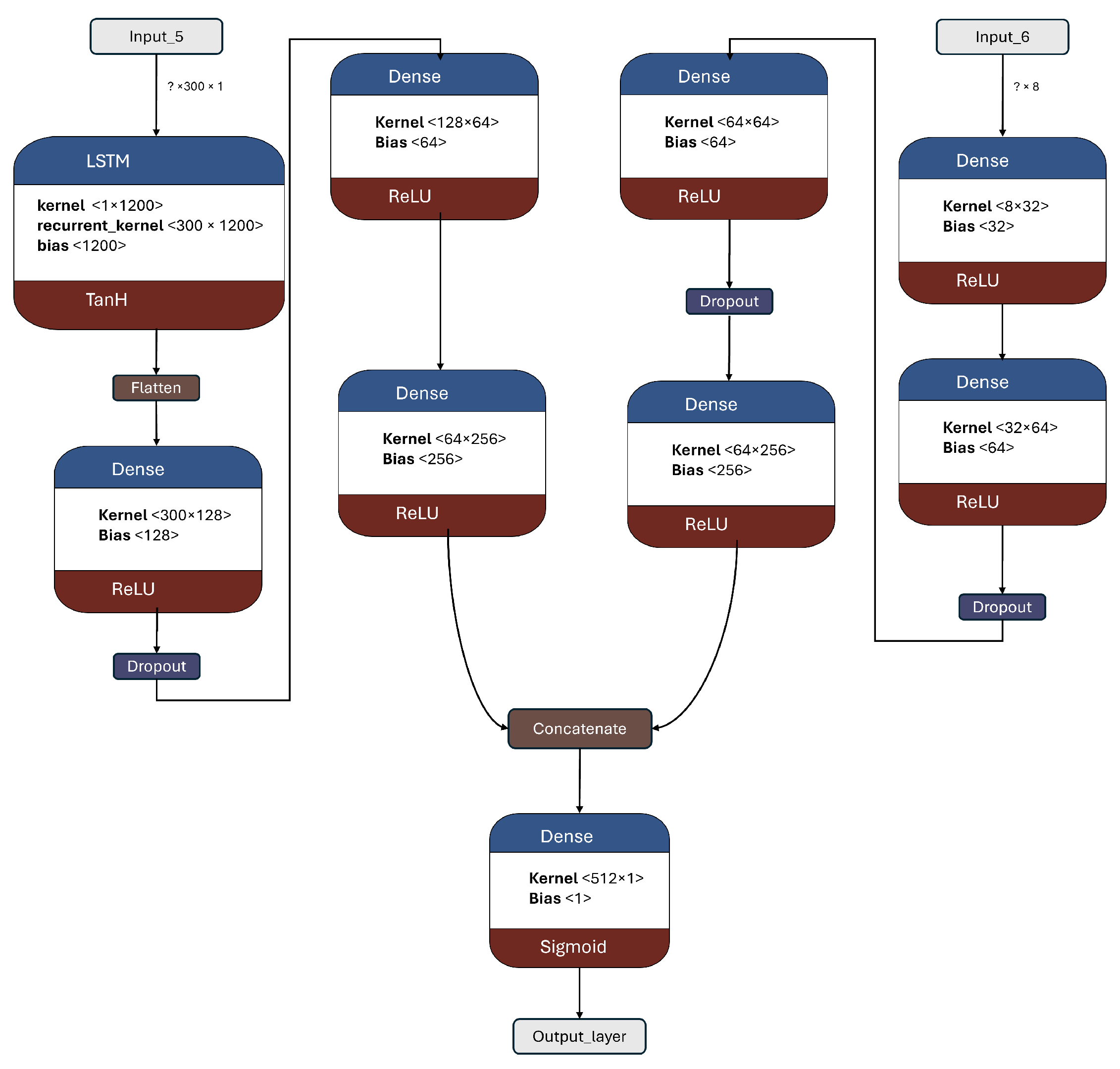
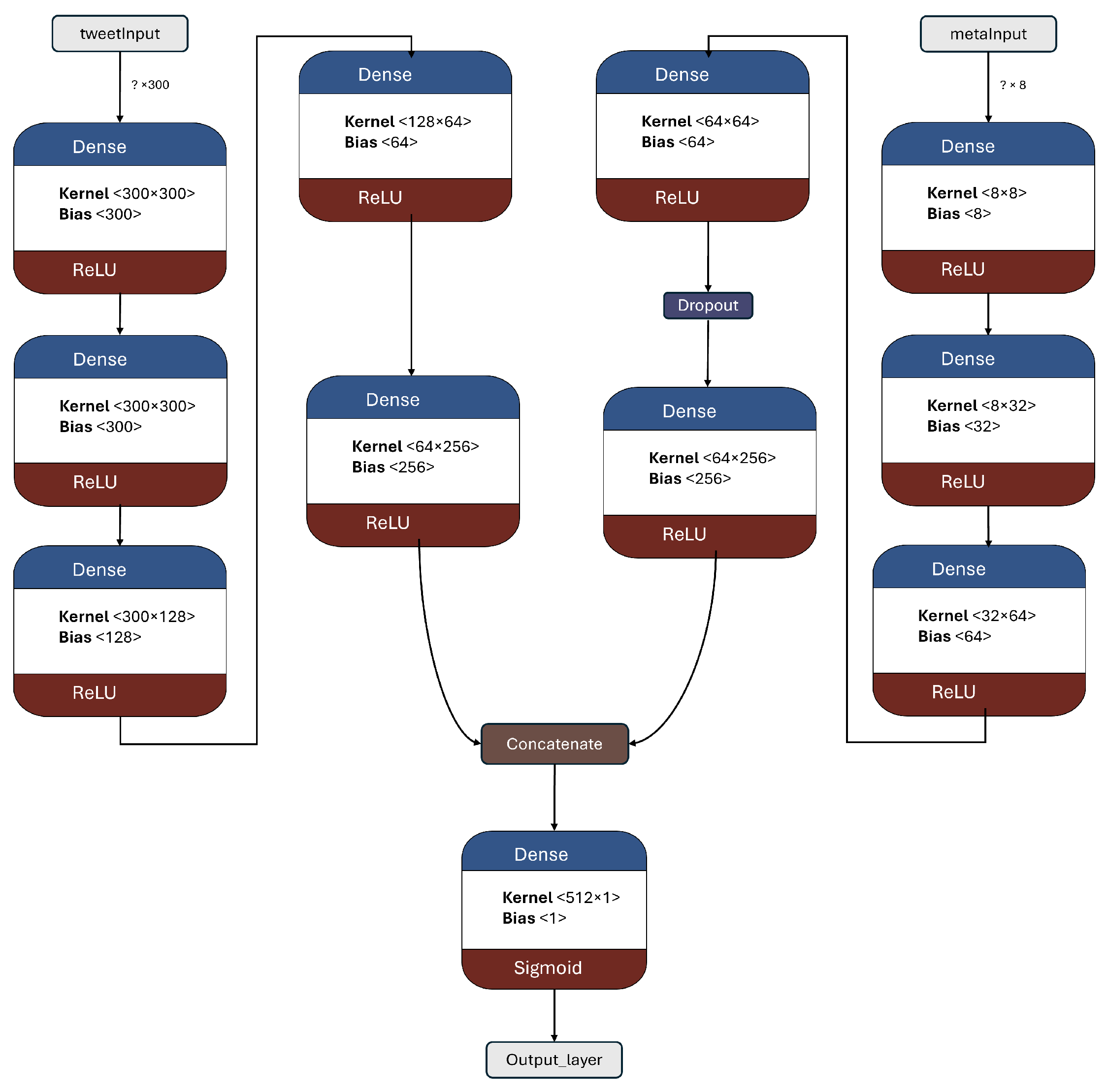
The architecture of the 2B1 model is presented in Figure 12. This model is the first two-branched model introduced in this work, with a total of 449,537 trainable parameters. The left branch takes the 300-dimensional tweet representation, which undergoes an LSTM layer [52] followed by a flatten layer to ensure a one-dimensional array as the next input. Subsequently, several dense layers and dropouts are applied. On the right branch, which receives the eight metadata features as input and passes them through a sequence of four dense layers with dropouts. The two branches are then merged using a concatenation layer, resulting in a one-dimensional output of size 512. Finally, the output layer produces the final prediction.

5.1.6. 2B2 Model

In this model, Dense layers are utilized in both branches to explore the possibility of replacing LSTM with a fully connected layer. The objective is to determine whether the model can still capture the main features and relationships within the text representation, or if its performance will deteriorate and become similar to random guessing.
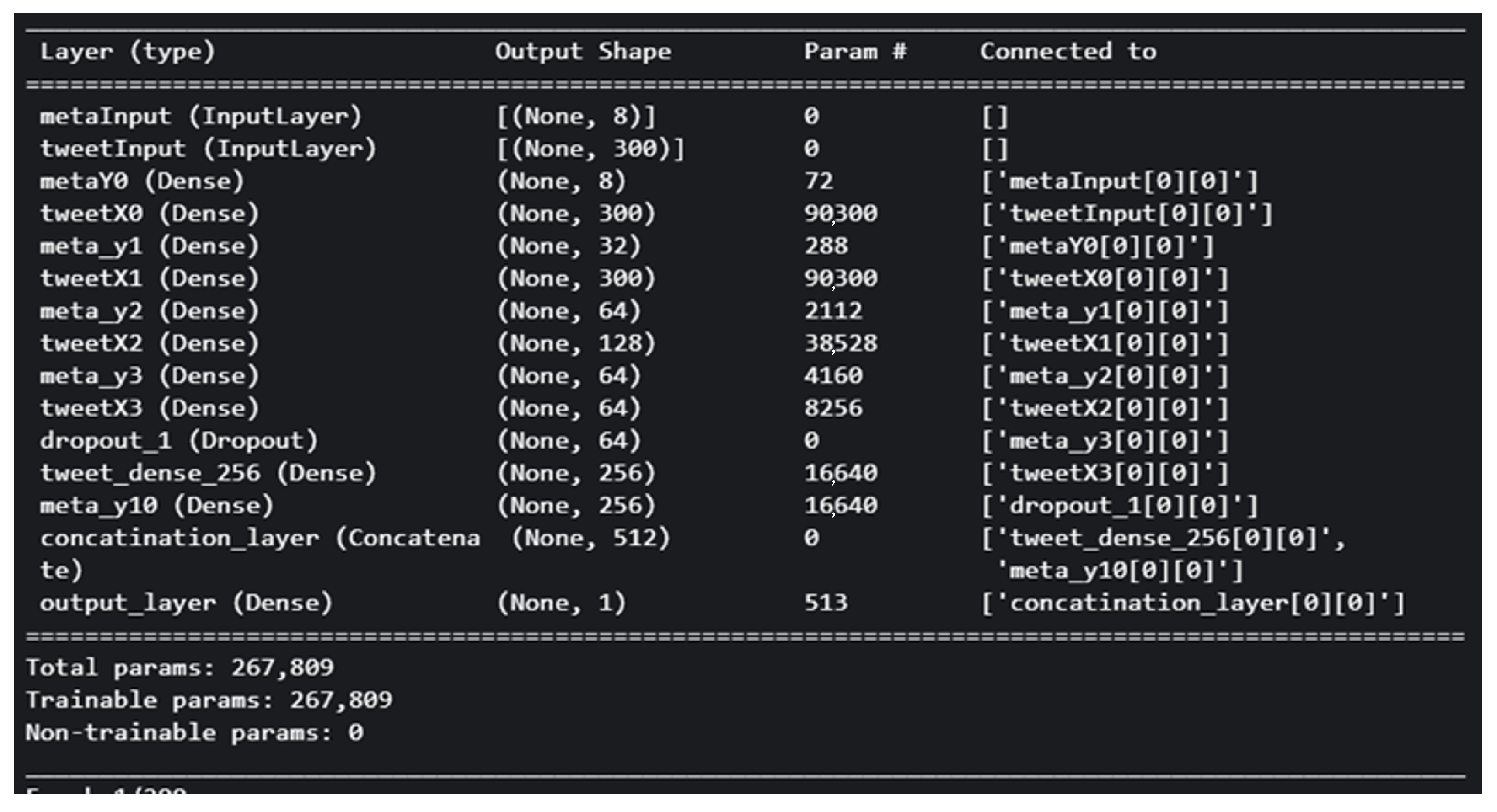
By substituting LSTM with Dense layers, the total number of trainable parameters reduces to 267,809. This modification also leads to a decrease in the training time and memory requirements. LSTM is known for being computational-intensive and is often recommended to be used in conjunction with a GPU and high RAM for efficient computation. The model architecture and summary are demonstrated in Figure 13. This visualization highlights the changes made to the model. In the tweet text branch, instead of using an LSTM layer, five dense layers are employed. Additionally, an extra dense layer is added to the right branch.

5.1.7. 2B3 Model

This model shares the same architecture and specifications as the 2B1 model (Figure 12), with the exception that all dropout layers have been removed. In some computer vision tasks, it has been shown that certain regularization techniques like weight decay and dropout may not be necessary when sufficient data augmentation is applied, challenging the conventional belief of their significance [57]. In this model, the objective is to explore the impact of removing all dropout layers, in this classification context. By eliminating dropouts, the aim is to understand how it affects the model’s performance and generalization capabilities.

6. Results and Discussion

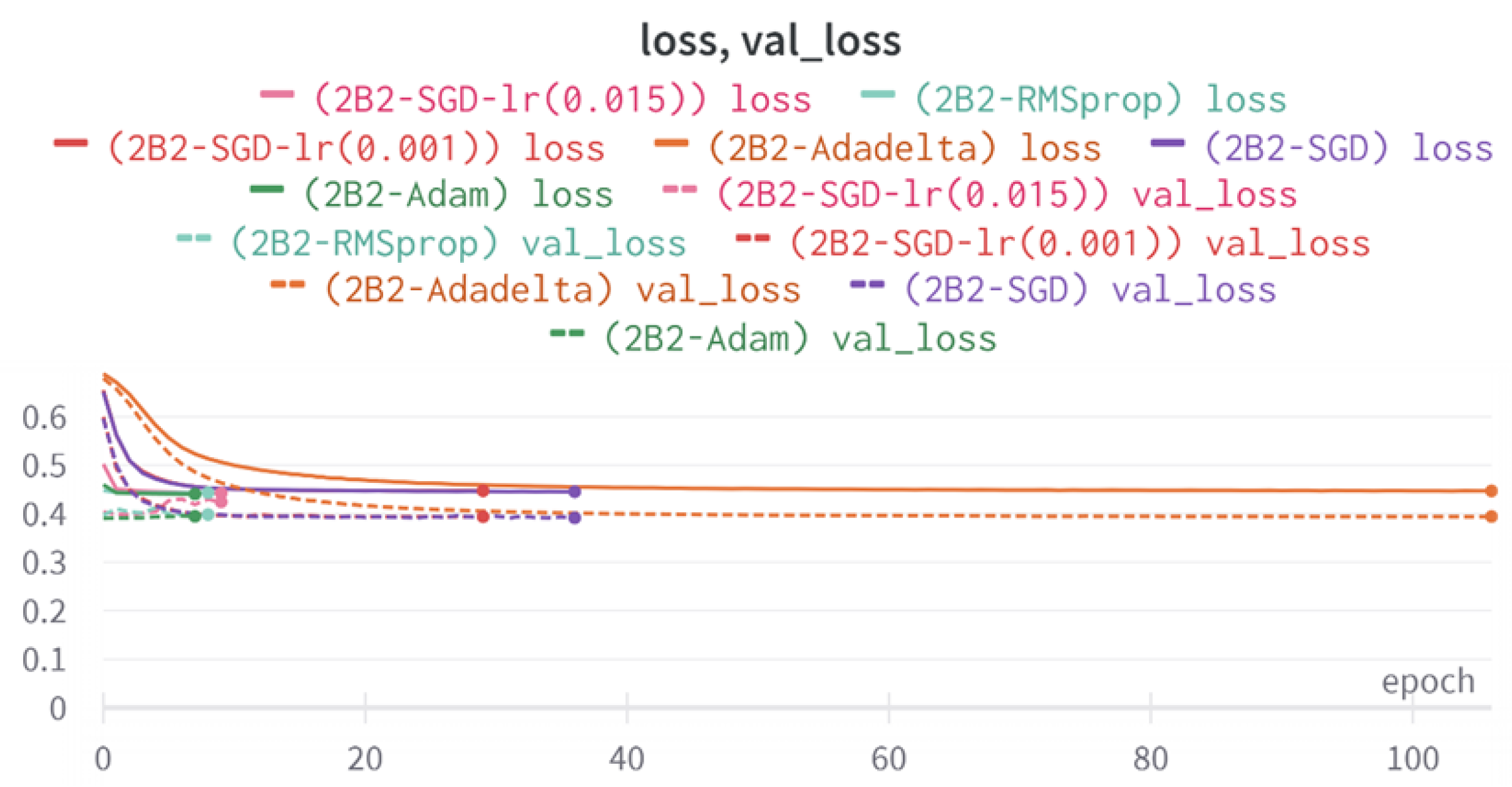
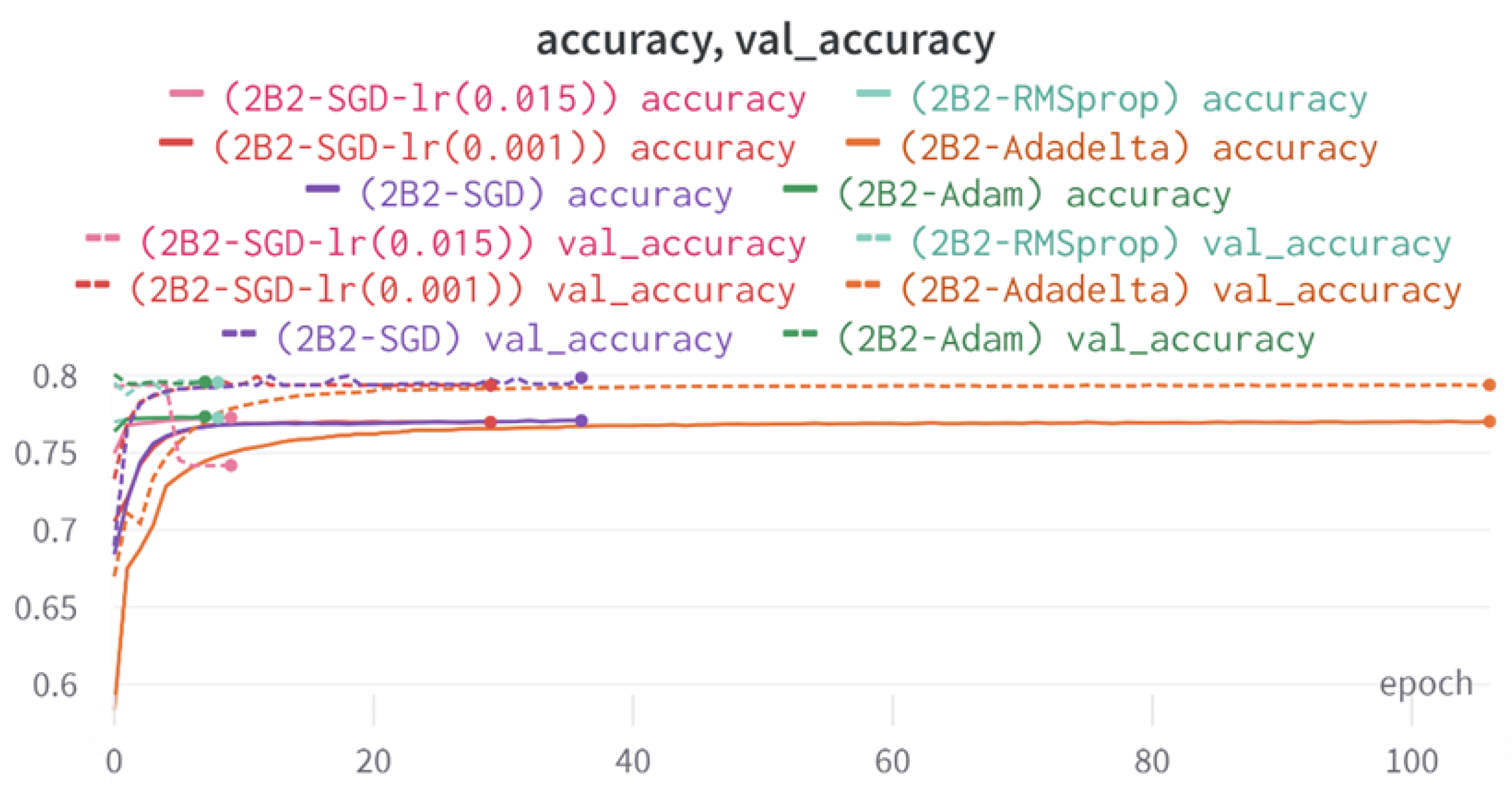
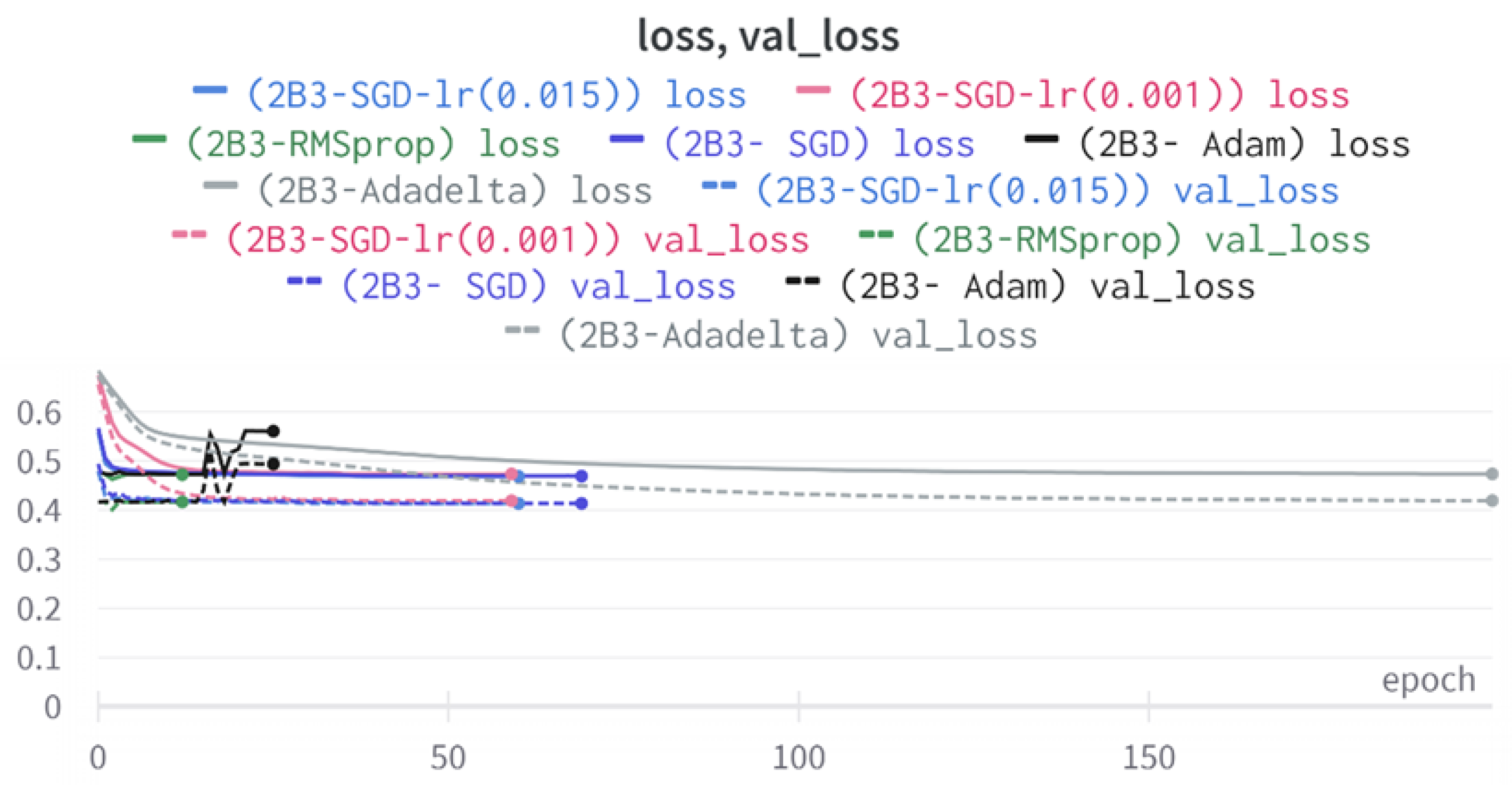
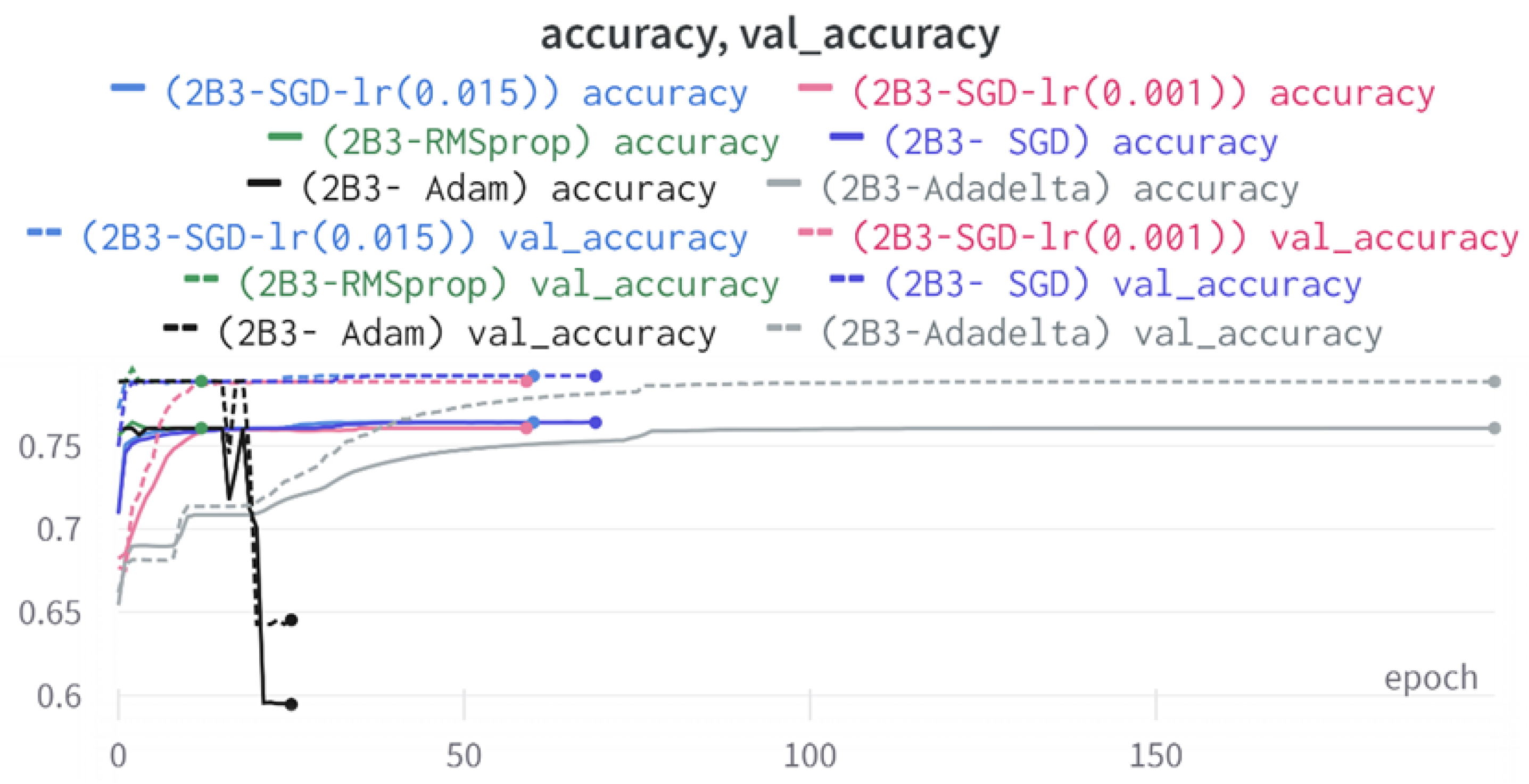
As mentioned earlier, models were monitored and saved on WandB and Google Colab Notebook [43]. Every model underwent training using four different optimizers, and in addition, two with a learning rate reducer. In this section, we present and discuss the results of each model. Several visualizations are provided, comparing accuracy, validation accuracy, loss, validation loss, and the confusion matrix for all five utilized optimizers. This approach provides and facilitates an effective comparison between different optimizers. In terms of evaluation metrics, the primary objective is to minimize the loss, false positives, and false negatives as much as possible, while maximizing all other relevant metrics. The training and accuracy plots serve as valuable tools for monitoring metric changes throughout the training process. These plots provide insights into various aspects of the model’s performance, such as determining if the model converges on the data and identifying potential instances of underfitting or overfitting.
In a well-fitted model, the training loss typically exhibits a consistent decrease throughout the training process, indicating effective learning and improved predictive performance. As training progresses, the loss should reach a stable level near the end. The validation loss, following a similar curve, is expected to be lower than the training loss. Regarding accuracy, the training accuracy generally increases at the beginning of training and stabilizes towards the end. The validation accuracy, although slightly lower, should also exhibit a similar trend.
Typically, since the model is optimized and learns from the training data, the training loss is expected to be lower than the validation loss, and the training accuracy is expected to be higher than the validation accuracy. However, it is important to note that this general expectation may not hold true in all cases, as the behavior of these metrics can vary depending on the specific dataset and model complexity. The split of the dataset also affects the whole process, as the classes considered by the model may not be well represented in the training and validation sets, and hence skewed data in the training or validation may lead to diverse results. This could be solved by applying stratified cross-validation, which guarantees a fair distribution of the data for effective testing and a reasonable outcome.
In the following, we summarize key trends across model families and optimizer behaviors, highlighting consistent patterns and notable anomalies. Full per-model results, including epoch-wise metrics, confusion matrices, and training curves, are provided in the (Appendixes Appendix A and Appendix B).

6.1. One-Branch Models (F1–F4)

All four one-branch architectures, which rely solely on user metadata, achieved remarkably consistent performance despite varying depth and regularization. Across optimizers, SGD consistently yielded stable convergence (72–79 epochs) with ≈79% accuracy, A U C 0.867 , and ≈0.595, while Adam frequently collapsed into trivial solutions. Notably, in F2-Adam and F3-Adam, it predicted nearly all samples as fake ( F P 0 , T N 0 ). RMSprop showed fast convergence but minor overfitting tendencies, and Adadelta often failed to stabilize within 200 epochs, sometimes producing high false positive rates (e.g., F4-Adadelta: FP = 21,922). Interestingly, increasing model depth ( F 1 F 3 ) or adding dropout (F4) did not significantly improve performance, suggesting that metadata alone contains sufficient signal for robust classification under this setup, and that architectural complexity offers diminishing returns.

6.2. Two-Branch Models (2B1–2B3)

The three two-branch models, which combine metadata with tweet embeddings, largely mirrored the performance of their one-branch counterparts, reinforcing the study’s central finding that tweet content adds limited value when fused via simple concatenation and encoded with SpaCy 300-d vectors. The best-performing model overall was 2B3-SGD, achieving MCC = 0.6007, a marginal gain over metadata-only models -while 2B2 (dense-only text branch) confirmed that shallow networks struggle to extract meaningful signals from static tweet embeddings. Again, SGD proved the most reliable optimizer, whereas Adam exhibited instability (e.g., 2B3-Adam: 100% recall but 58% precision due to aggressive false positives). Notably, removing dropout (2B3) did not degrade performance, suggesting that data augmentation may partially substitute for explicit regularization in this context. Overall, the multimodal architectures did not outperform metadata-only baselines in a statistically meaningful way, underscoring the dominance of metadata features in this experimental framework.

6.3. Discussion

In this study, multiple models were trained using different optimizers, revealing significant performance disparities tied to architectural and data-related vulnerabilities. It should be noted that augmented samples were included in both training and test sets. While this was intended to evaluate robustness under diverse synthetic scenarios, it deviates from standard practices and may have led to optimistic performance estimates, a pattern reflected in the recurrent anomaly of validation loss falling below training loss. While the SGD optimizer consistently demonstrated robust convergence and accuracy, Adam exhibited instability, particularly in models like F2-Adam, F3-Adam, and 2B3-Adam, where it collapsed into trivial solutions (FP = 0, TN = 0) due to sensitivity to skewed gradients. RMSprop and Adadelta performed moderately but struggled with architectures prone to overfitting, such as F4-Adadelta, which misclassified 21,922 legitimate accounts as fake (FP approximately 42% of TP). This could be caused by amplified noise in augmented data.
The observed anomaly of validation loss remaining persistently lower than training loss -most pronounced in F4-Adadelta and 2B1-SGD-LR (0.015) suggests data leakage during augmentation, where synthetic samples mirrored training patterns, or flawed stratification skewed class representation. For instance, metadata-only suffered from overlapping features between highly active legitimate accounts and fake accounts, while some two-branched models failed to harmonize tweet embeddings with metadata, resulting in erratic loss curves. Notably, models lacking dropout, such as 2B3-Adadelta, overfit to honeypot-specific features, and architectures relying on Adam, like F3-Adam, degenerated into predicting all samples as one class, highlighting optimizer-induced problems. These patterns underscore the fragility of deep learning frameworks in detecting fake accounts, where optimizer choice, data representativeness, and feature diversity critically mediate performance. To address these issues, future work should prioritize stratified cross-validation to ensure balanced class representation, refine data augmentation to avoid synthetic biases, and replace unstable optimizers like Adam with SGD or RMSprop in architectures prone to collapse.
The F4-Adadelta model’s extreme FP count (21,922) and TN (30,581) reflect a failure to distinguish nuanced metadata patterns, likely exacerbated by the Social Honeypot dataset’s synthetic biases, which disproportionately represented bot-like behaviors. Similarly, F2-Adam’s near-zero FP and TN values (FP = 1, TN = 52,502) reveal a collapse into trivial solutions, where the model prioritized minimizing loss by ignoring class boundaries entirely. This behavior aligns with Adam’s susceptibility to gradient noise in imbalanced datasets, a flaw less pronounced in SGD’s fixed learning rate. Meanwhile, 2B3-SGD ’s superior MCC (0.6007) underscores the value of combining tweet embeddings with metadata. The F1-Adadelta model’s prolonged training (199 epochs) without convergence suggests that adaptive optimizers like Adadelta may require stricter early stopping criteria or dynamic learning rate schedules to avoid overfitting to augmented data.
The persistent issue of validation loss dipping below training loss across models points to systemic flaws in data partitioning. Augmented samples from the Social Honeypot dataset, designed to mimic real-world spam, may have inadvertently mirrored training data, creating an artificial overlap between training and validation sets. This overlap allowed models to exploit synthetic patterns rather than generalize. For example, F4-Adadelta ’s high FP rate (42% of TP) likely stemmed from overemphasizing follower ratios, a feature easily manipulated in honeypot data.
The F3-Adam, F2-Adam, and F4-Adam models’ inability to converge, halting after 7–9 epochs, illustrates Adam’s instability in sparse-feature environments. Metadata features like “listed count” or “favorites count,” which lack clear discriminatory power, may have produced noisy gradients, destabilizing Adam’s adaptive learning rate. In contrast, SGD’s fixed rate allowed gradual convergence in models like 2B3-SGD, which balanced tweet and metadata signals effectively. The 2B2-SGD model’s reliance on dense layers for tweet processing, instead of LSTM, highlights another limitation: shallow networks struggle to model sequential dependencies in text, reducing tweet data’s utility. This aligns with the study’s broader finding that combining modalities (text + metadata) did not always boost performance, likely due to suboptimal feature fusion and insufficient text preprocessing.
It is important to note that our findings, showing that tweet content provides limited improvement over metadata alone, are contingent on our specific design choices: (1) the use of static SpaCy word vectors for tweet representation, which lack contextual awareness compared to transformer-based embeddings, and (2) a simple concatenation-based fusion strategy that does not model cross-modal interactions. More recent works like [29] have demonstrated that advanced fusion mechanisms -such as gated units or attention, can better exploit complementary signals between text and metadata. Therefore, our results should not be interpreted as evidence that tweet content is inherently uninformative, but rather that its utility depends critically on the quality of text encoding and fusion architecture.
Finally, the F1-SGD-LR (0.001) model’s erratic learning rate reduction (from 0.001 to 1.5 × 10⁻⁷) without performance gains underscores the need for adaptive scheduling tailored to dataset characteristics. Overly aggressive rate decay may have trapped the model in shallow local minima, while insufficient decay in F4-SGD-LR (0.001) prolonged training without improving generalization. These findings collectively emphasize that robust fake account detection requires not only sophisticated architectures but also careful optimizer selection, data curation, and validation strategies to mitigate biases and synthetic artifacts inherent in augmented datasets.

7. Conclusions and Future Works

This work manifests the significance and widespread influence of social media, along with its implications and potential threats. It specifically emphasizes the importance of identifying abnormal actors on social media platforms. The study’s main focus is on the detection of fake accounts on Twitter using a binary classification approach. Through an extensive review of related works and surveys, various approaches and techniques employed in previous studies are examined, while also highlighting the significant limitations and drawbacks present in the current literature that this study aims to overcome. Overall, the shortcomings of the related work include limited scope, dependency on historical data, potential evasion by fraudulent actors, costly implementation, lack of comprehensive features, limited generalizability, lack of comparative analysis, and incomplete coverage of spam detection. By recognizing and addressing these limitations, this study seeks to contribute to the advancement of fake account detection on social media platforms, particularly on Twitter. While our approach does not match the architectural complexity or input modality richness of recent state-of-the-art frameworks, it offers a lightweight, reproducible, and deployment-friendly alternative that achieves competitive performance using only user metadata and raw tweet text -without requiring graph construction, external APIs, or extensive computational resources. To tackle the problem, a dataset was collected and carefully prepared from diverse sources and perspectives. To cover a wide range of real-life scenarios, data augmentation techniques were applied. The dataset was structured into two formats, aligning with the requirements of two types of models. The first format consisted of user metadata alone, while the second format incorporated both user metadata and one of their tweets. This approach, which combines numerical and textual data, has been found to be more efficient in this particular task, according to several studies.
Drawing upon deep learning techniques, seven different architectures were proposed and implemented. These models were tested using four different optimizers: SGD, RMSprop, Adam, and Adadelta. Furthermore, to explore the impact of the learning rate, models utilizing the SGD optimizer were trained twice, incorporating a learning rate reducer. The implemented models comprised four single-branched models that utilized only user metadata, and three two-branched models that incorporated both user metadata and tweets.
To assess the performance of each model, a range of metrics were employed, including loss, accuracy, area under the curve (AUC), confusion matrix, precision, recall, specificity, F1 and F2 scores, and the Matthews Correlation Coefficient (MCC). These metrics offered comprehensive insights into the models’ performance and effectiveness in classification tasks. Contrary to the claims made previously, the incorporation of tweets alongside user metadata did not significantly impact the models’ ability to classify fake accounts. The SGD optimizer consistently demonstrated good performance, while RMSprop and Adadelta also yielded favorable results in certain models. However, the Adam optimizer exhibited unstable behavior and struggled to converge.
Overall, SGD emerged as the most efficient optimizer in the majority of cases, whereas Adam showed comparatively less effectiveness. It is crucial to focus on optimizing the learning rate and closely monitor metrics such as loss, accuracy, and convergence during training. In general, the results indicated that SGD optimizers and learning rate reducers showed promising outcomes in most cases, while RMSprop and Adam optimizers exhibited some issues. Adadelta performed well in certain models but had its limitations.
Considering the similarities observed in the results of this study and the scope for improvement, several avenues for future work can be explored, including:
  • exploring additional datasets and features: incorporating diverse datasets and additional features may enhance the accuracy and robustness of classification.
  • Conduct feature importance analysis (e.g., SHAP, LIME) to quantify the contribution of individual metadata and textual features to model predictions.
  • Re-evaluate all models on a strictly unaugmented test set to obtain unbiased generalization metrics.
  • Implement stratified, grouped K-fold cross-validation (grouped by user account) to ensure robust performance estimation and quantify fold-level variance.
  • Generalization to different platforms: Extend the study to encompass multiple social media platforms, as each platform may have unique characteristics and challenges regarding fake account detection. Investigate the transferability of the models and their performance on different platforms.
  • Investigate the use of more advanced deep learning architectures, such as transformers, and how such architectures can improve classification performance.
  • Explore transformer-based text representations to assess whether richer semantic encoding can unlock the value of tweet content in multimodal fake account detection.
  • use of transfer learning: by using some pretrained models on some related tasks in the domain of fake account detection. This may leverage existing models and improve their performance.
  • Additional training and fine-tuning: Focus on further refining the proposed models that exhibit a good fit and classification ability. Emphasize additional training and fine-tuning strategies, particularly for models that have successfully converged and completed all training epochs without reaching a fixed and stable loss.
  • Conduct repeated experiments across multiple random seeds to compute confidence intervals for all metrics, and include strong non-deep-learning baselines (e.g., XGBoost, Random Forest) for comprehensive comparison.
  • Exploring advanced synthetic data generation methods, such as GANs or diffusion-based models for simulating evolving fake account behaviors to enhance dataset diversity and model robustness against emerging threats.
  • Evaluate model robustness via cross-dataset testing, and ablate provenance-sensitive features to isolate generalizable signals.
  • Explore emerging representation learning paradigms, such as state-space sequence models (e.g., DyG-Mamba [58,59]) and dynamic graph clustering techniques [60,61] for enhanced modeling of temporal and relational patterns in social media accounts.
  • Extend the framework to incorporate visual modalities, such as profile pictures and posted images, using CNN and transformer-based architectures for image analysis and segmentation (e.g., [62,63]).
By pursuing these future directions, the field of fake account detection can continue to advance, leading to more effective and reliable approaches for identifying non-real human actors on social media platforms.
Author Contributions

All authors (Z.E., K.E. and R.A.) contributed equally to all aspects of this work, including conceptualization, methodology, software, validation, formal analysis, investigation, resources, data curation, writing—original draft preparation, writing—review and editing, visualization, supervision, project administration, and funding acquisition. All authors have read and agreed to the published version of the manuscript.

Funding

This research received no external funding.

Institutional Review Board Statement

Not applicable.

Informed Consent Statement

Not applicable.

Data Availability Statement

The datasets used in this study are publicly available at: http://mib.projects.iit.cnr.it/dataset.html (accessed on 11 November 2025) and https://www.kaggle.com/datasets/ziadelgammal122/twitter-fake-accounts (accessed on 11 November 2025).

Conflicts of Interest

The authors declare no conflicts of interest.

Appendix A. Per-Model Results

Appendix A.1. F-1 Model

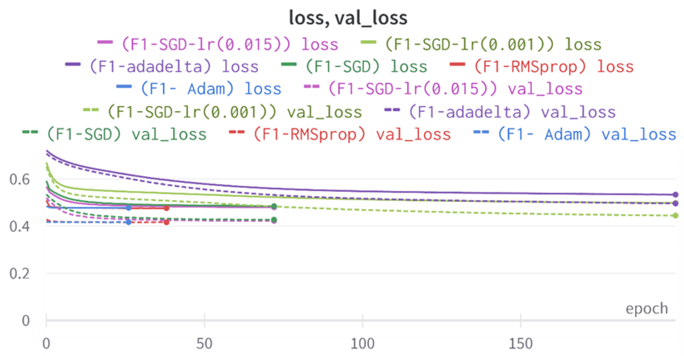
The results of different models and optimizers of F1 architectures are summarized in Figure A1 and Figure A2. Table A1 shows the evaluation metrics of each model after testing it on the unseen data. Figure A1 illustrates how the loss and validation loss evolve during the training process.
Figure A1. F1 models loss, validation loss.
Bdcc 09 00298 g0a1
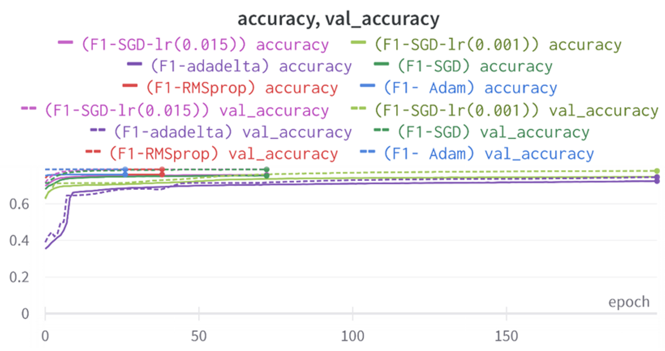
Figure A2. F1 models accuracy, validation accuracy.
Bdcc 09 00298 g0a2
Figure A2 also shows how the accuracy and validation accuracy change for these six models. Despite having the fewest number of parameters(321) and being the simplest model implemented in this study. This model provides some satisfactory results that are even better than other, more complicated and complex models. F1-SGD model halted training after 72 epochs due to early stopping, achieving an accuracy of 79% and an AUC of 0.866. According to the confusion matrix in Figure A15, the majority of the predicted instances fall within the range of 34,953 true positives and 47,756 true negatives. However, there were 17,476 instances that were classified incorrectly as false negatives and 4747 instances that were classified incorrectly as false positives. Looking at the evolution of loss, validation loss, and accuracy, validation accuracy for this model will illustrate that the model effectively adapts to the data and converges.
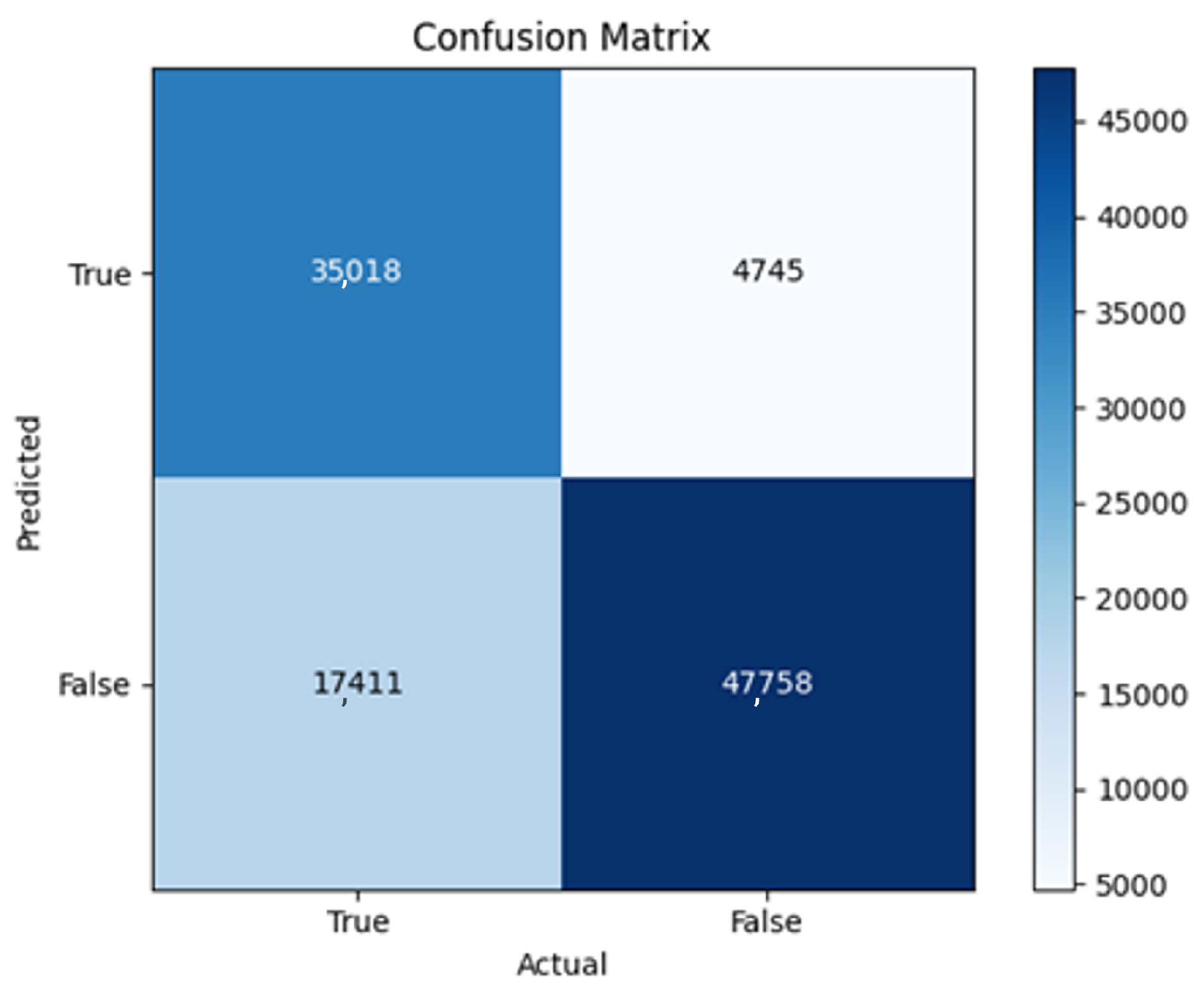
In F1-RMSprop, the training process was terminated after 38 epochs due to early stopping. The CM in Figure A16 revealed that this model exhibits higher values of 35,018 true positives and 47,761 true negatives. Additionally, 4742 false positives were in close proximity, while the false negatives decreased to 17411. According to the loss plot, there is an increased gap of approximately 0.06 between the loss and validation loss compared to the F1-SGD model. However, despite this larger gap, the model exhibits faster convergence, and the loss begins to stabilize even before reaching the tenth epoch of training. As these results show, most of the metrics are quite similar to the F1-SGD model. The loss is slightly lower, which explains the slight improvement in the CM and some other metrics like the AUC, F1 score, F2 score, and MCC.
The results of the F1-Adam model are quite similar to F1-RMSprop, with a 0.001 increase in the loss and some very small changes in the TN and FP as shown in the CM in Figure A17. The loss figure reveals a noticeable pattern when using the Adam optimizer. The loss fails to minimize or stabilize, and the validation loss displays fluctuating behavior. As a result, the training process was halted after only 26 epochs. Interestingly, the validation accuracy remains constant throughout all training epochs. These observations strongly suggest that the issue is primarily related to the optimizer itself or initialized weights, as these were the only variables altered in this scenario.
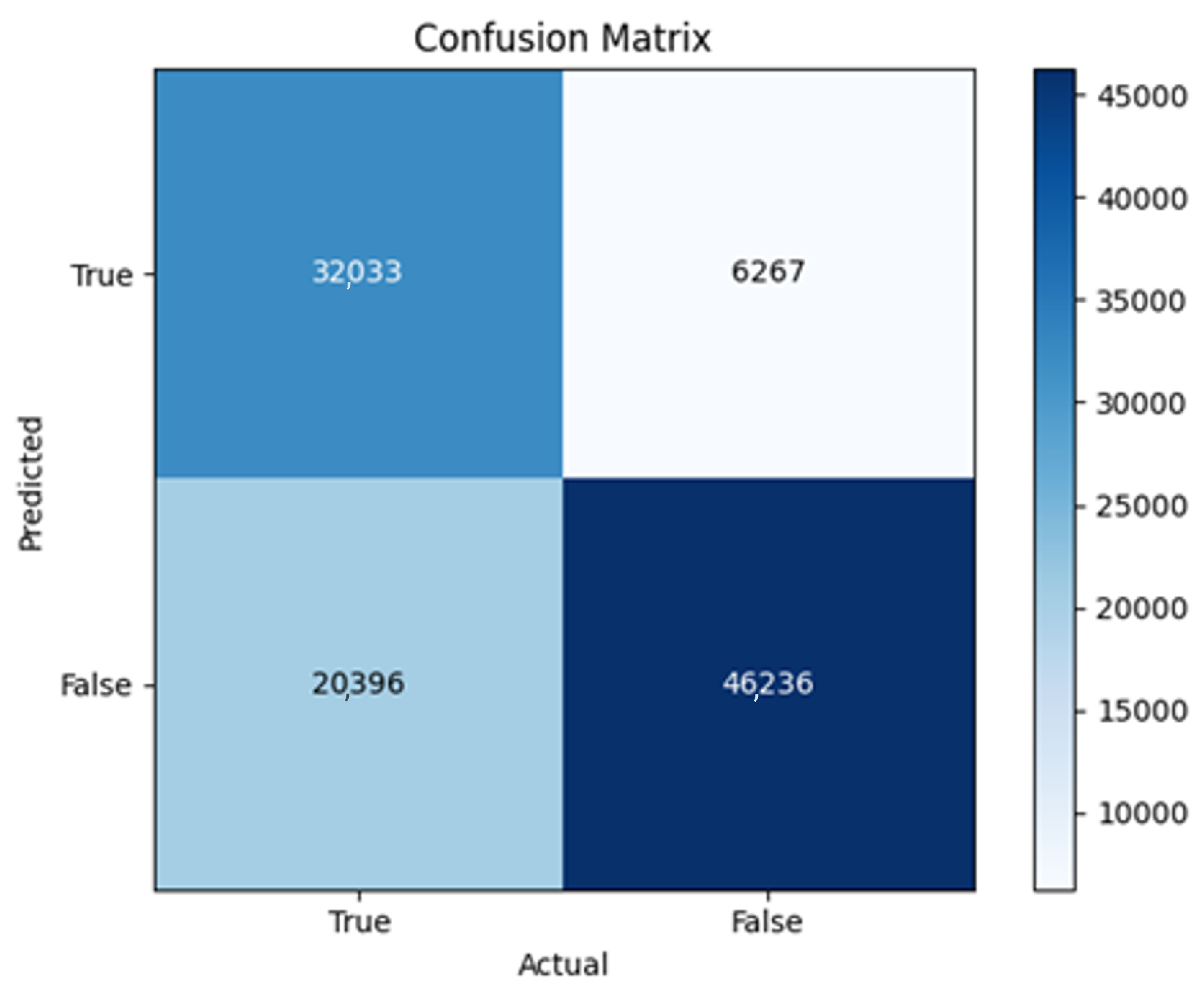
F1-Adadelta underwent the entire 200 pre-defined training epochs without any intervention by early stopping. Figure A18 depicts the confusion matrix of this model.
During the training process, the loss consistently decreased; however, it did not reach a stable level by the end. This suggests that further training and tuning may potentially improve the model’s performance. In F1-SGD-LR (0.015), applying the learning rate reducer with 0.015 as initial learning rate, the value decreased down to 0.00001500. The training halted after 72 epochs, achieving an accuracy of 79% and AUC of 0.867, and the loss value was 0.423.
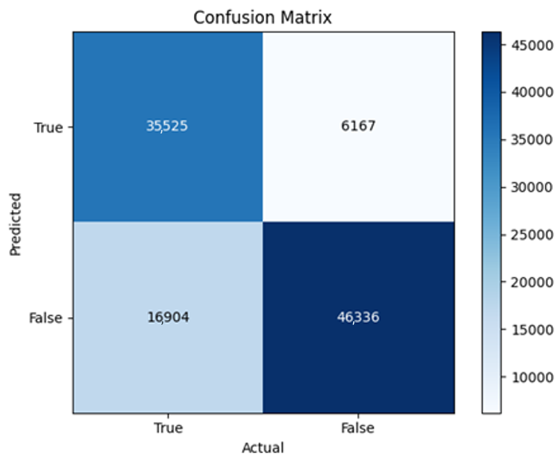
Despite the application of a learning rate reducer in F1-SGD-LR (0.0010), the learning rate value remained constant at 0.0010 throughout all the epochs, indicating that the reducer did not modify the learning rate. The model’s accuracy experienced a decline of 1 percent, reaching a final accuracy of 78%. Interestingly, the loss with a value of 0.445 was the second highest observed in this architecture. Just like the F1-Adadelta model, the training process successfully completed all 200 epochs without any early stopping. According to the confusion matrix shown in Figure A20, this model performed exceptionally well in identifying true positives, representing the fake accounts. It achieved the highest number of true positives (TP) among all the F1 models. Additionally, the number of true negatives (TN) slightly decreased to 46336. In terms of false negatives (FN), this model had the lowest count compared to the other four optimizers. However, the number of false positives (FP) increased to 6167.
Based solely on the confusion matrix results, it can be concluded that this model outperforms the other F1 models. It successfully identified the highest number of fake accounts correctly (TP) and had the lowest number of false positives (FP) among other F1 models.
Table A1. F1 Results.
NameepochsAccLossAUCTPTNFPFNPrecisionRecallSpecificityF1F2MCC
F1-SGD720.790.4280.86634,95347,756474717,4760.8810.6680.910.7590.70.5941
F1-RMSprop380.790.4160.86835,01847,761474217,4110.8810.6680.910.760.7020.5953
F1-Adam260.790.4170.86835,01847,759474417,4110.8810.6680.910.760.7020.5953
F1-Adadelta1990.750.4960.82532,03346,236626720,3960.8360.6110.8810.7060.6460.5106
F1_SGD-lr (0.015)720.790.4230.86735,00047,755474817,4290.8810.6680.910.7590.7020.5949
F1- SGD-lr (0.001)1990.780.4450.85835,52546,336616716,9040.8520.6780.8830.7550.7070.5723

Appendix A.2. F-2 Model

Despite the inclusion of additional densely connected layers, expected to enhance its ability to capture interconnected relations among various features, the results contradicted this intention. Surprisingly, the performance of the majority of F-2 models was almost equal to that of the simpler F-1 model. Figure A3 and Figure A4, and Table A2 summarize the results.
Figure A3. F2 models loss, validation loss.
Bdcc 09 00298 g0a3
Figure A4. F2 models accuracy, validation accuracy.
Bdcc 09 00298 g0a4
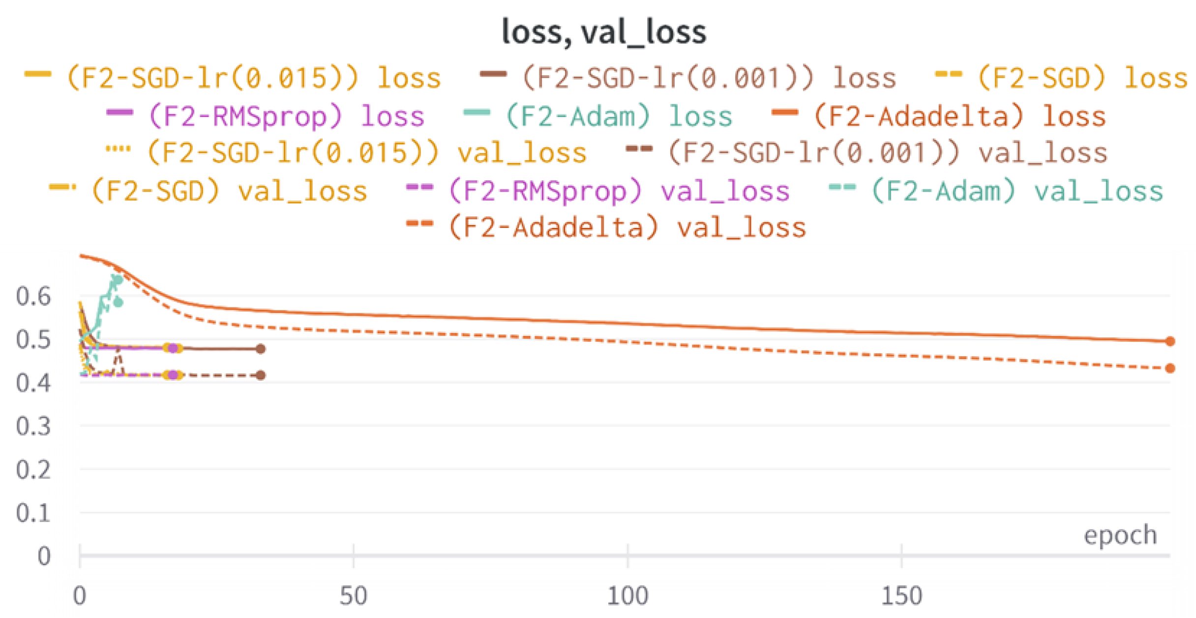
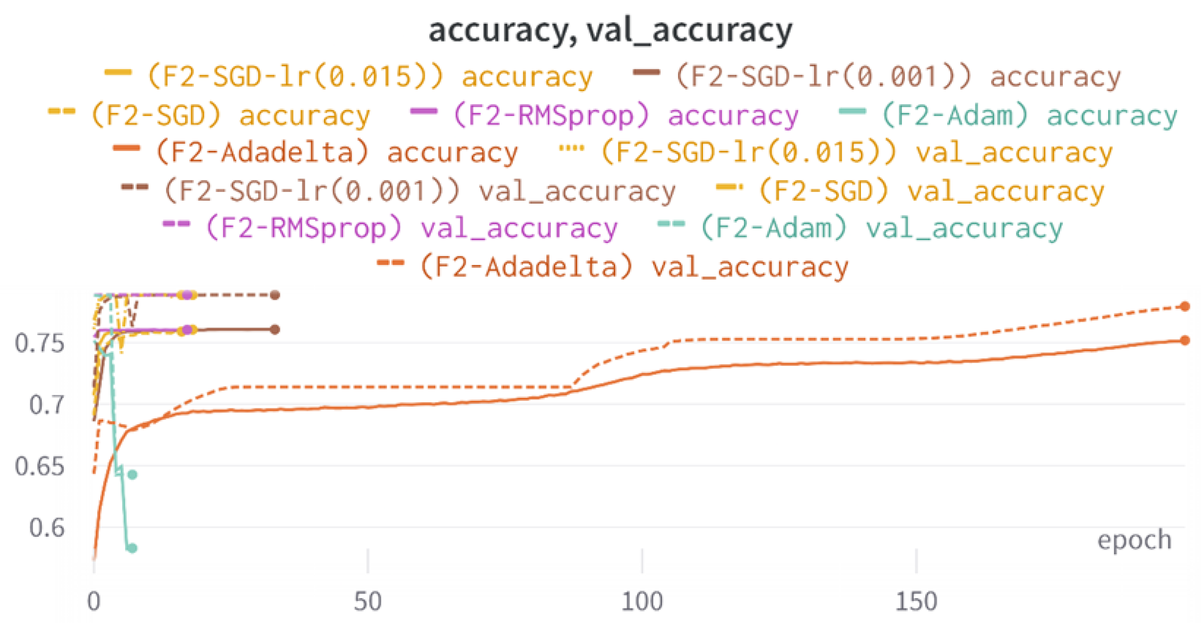
Early stopping halted the training for Most of the F2 models; Figure A3 shows that F2-SGD was the first one to halt training after 16 epochs. While F2-Adadelta was the only one to complete the full 200 training epochs.
In the F2-RMSprop model, the loss remains relatively stagnant after the initial 2 epochs, which can be seen in the loss and accuracy plots.
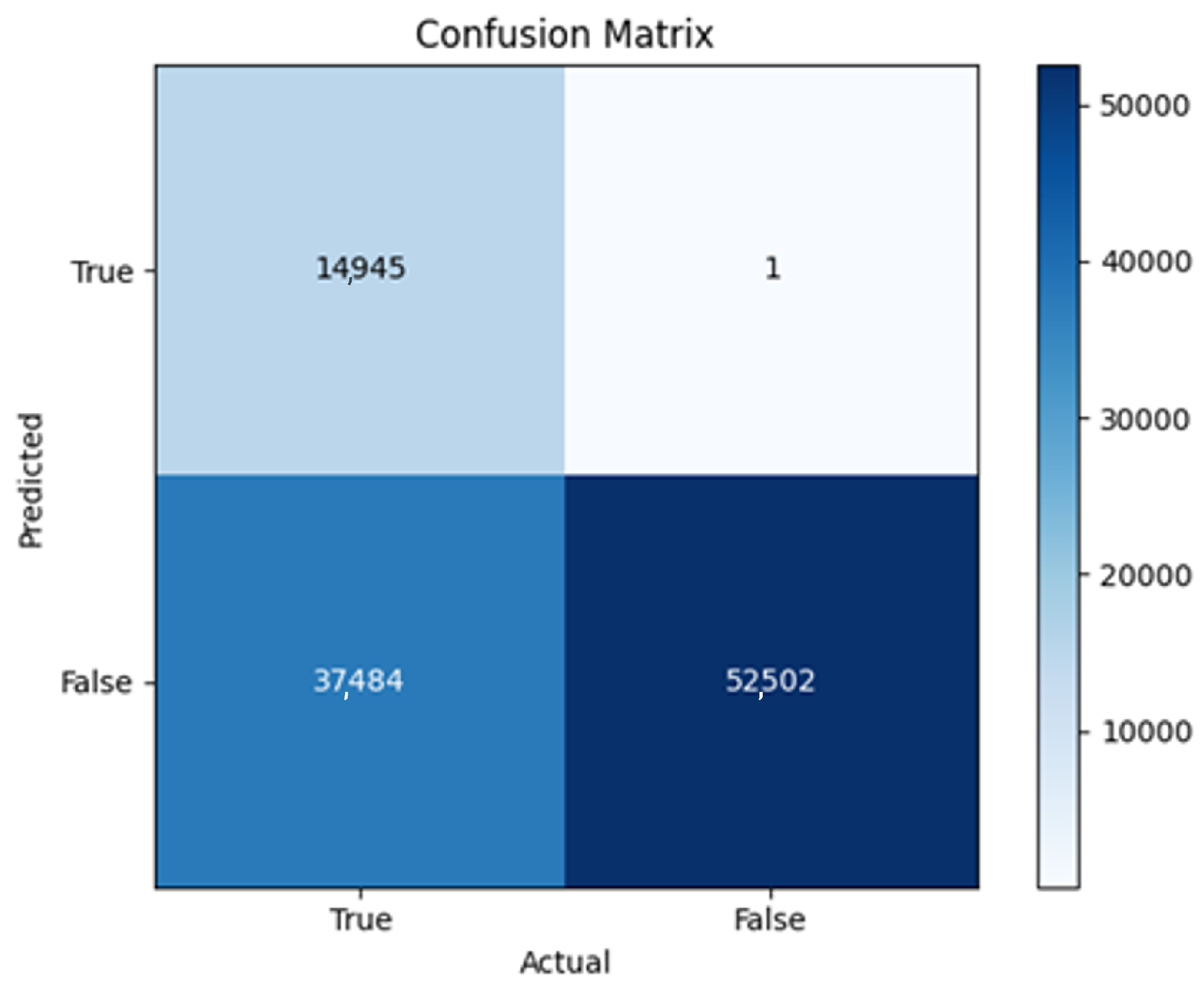
This observation may indicate a potential issue of overfitting, suggesting that the model has reached a point where it is unable to effectively learn from the data and generate generalized rules. F2-Adam shows an unusual behavior; looking at the confusion matrix, we find a very low number of false positives (just 1). On the other hand, the false negatives (FN) increased to 37484. The true positives (TP) also decreased, from the average of other models to 14945. However, another noticeable value was the large increase in the number of true negatives to 52502. However, when looking at the unstable increasing loss and decreasing accuracy for this model, in addition to the early stopping of the training after only 7 epochs, this implies the same issue that the model is not able to generalize and learn from the data. The reason behind this instability or inability to converge that always comes with models using the Adam optimizer (as will be shown in the rest of the results)can be attributed to its adaptive learning rate; while being efficient in theory, it led to unstable training dynamics and caused the model to fall into some trivial solutions like predicting a single class.
Between all F2s, F2-SGD-LR (0.015) and F2-SGD-LR (0.001) have the lowest loss. With the use of learning rate reducer in F2-SGD-LR (0.015), the learning rate went down to 0.0015, and in F2-SGD-LR (0.001). All the results obtained from F2-models are summarized in Table A2, and confusion matrices can be found in the appendix (Figure A21Figure A26).
Table A2. F2 Results.
NameepochsAccLossAUCTPTNFPFNPrecisionRecallSpecificityF1F2MCC
F2-SGD160.790.4170.86635,01847,753475017,4110.8810.6680.910.760.7020.5951
F2-RMSprop170.790.4170.86835,01847,759474417,4110.8810.6680.910.760.7010.5953
F2-Adam70.640.5840.64314,94552,502137,4840.10.2850.10.4440.3320.4078
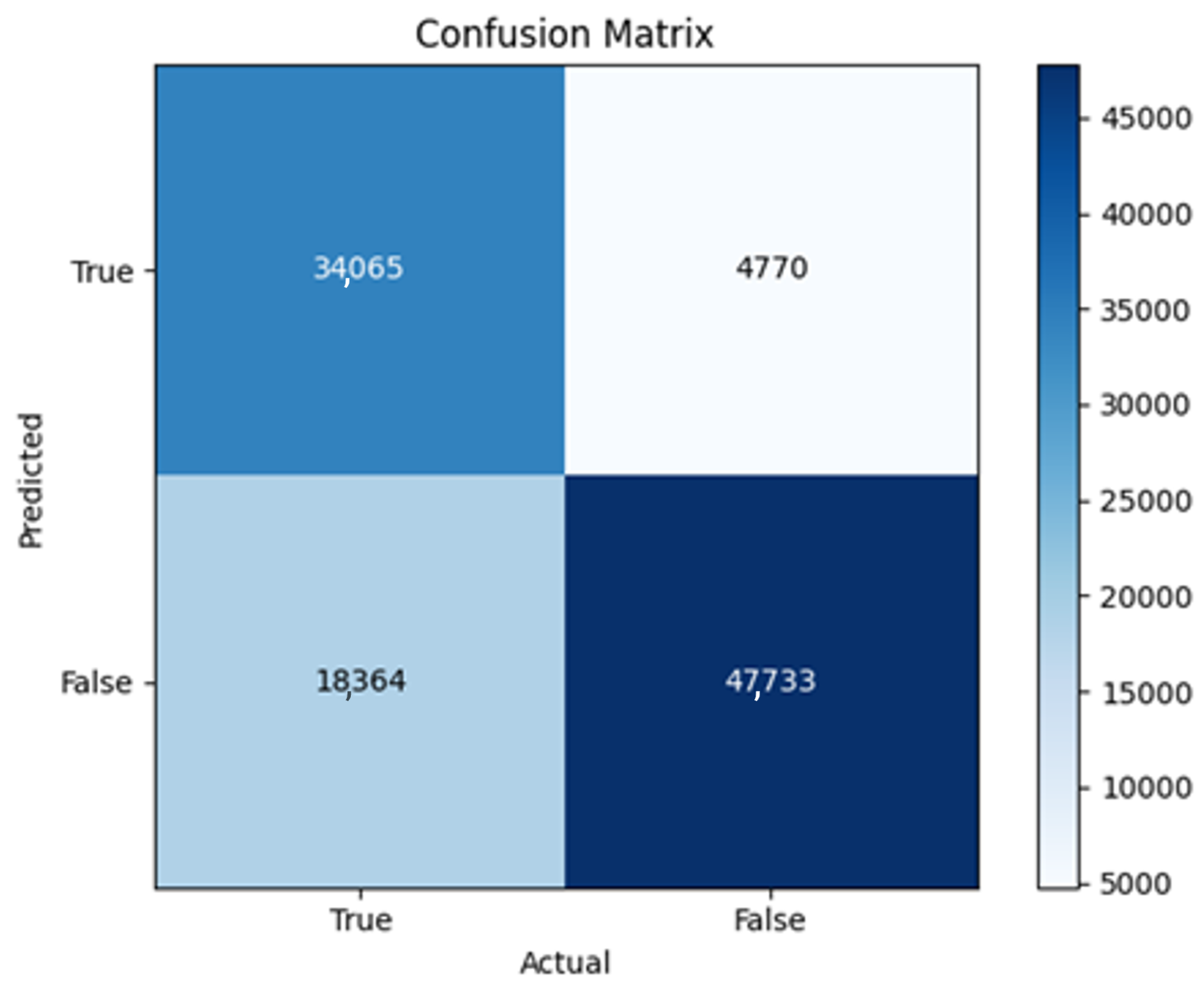
F2-Adadelta1990.780.4320.8634,06547,733477018,3640.8770.6450.9090.7470.6850.5788
F2-SGD-lr (0.015)180.790.4160.86835,01847,758474517,4110.8810.6680.910.760.7020.5952
F2-SGD-lr (0.001)330.7890.4160.86835,01847,760474317,4110.8810.6680.910.760.7010.5953

Appendix A.3. F-3 Model

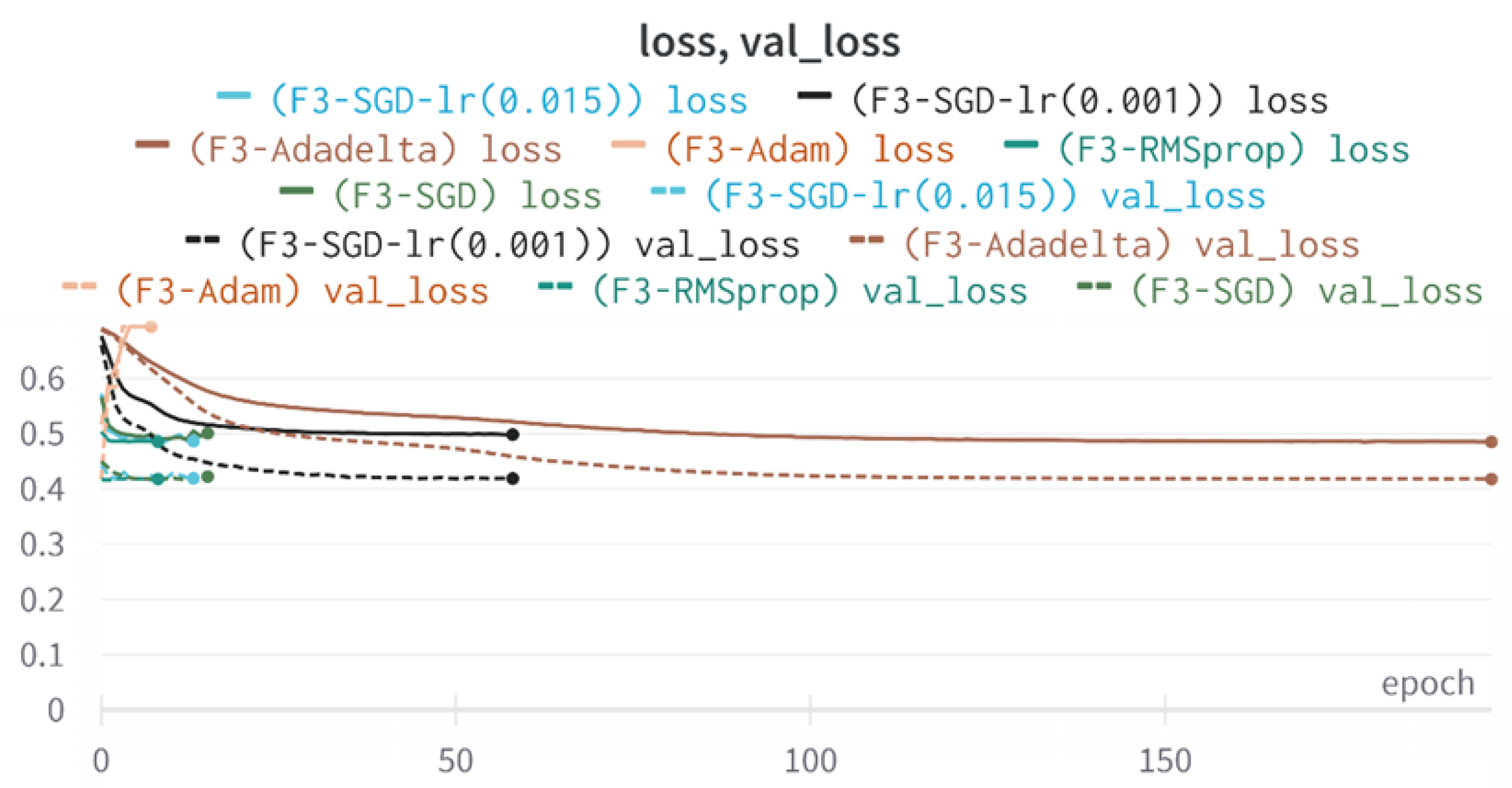
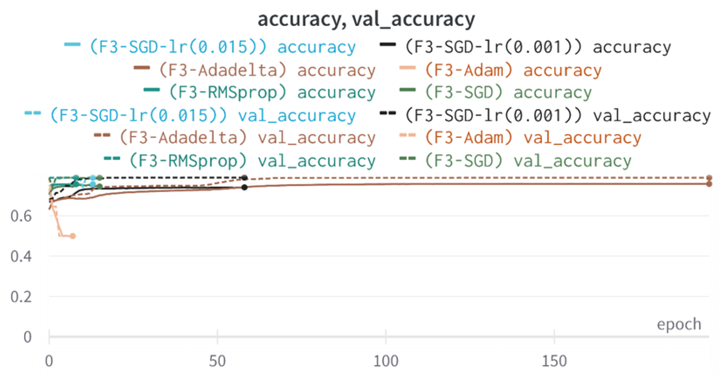
Out of the various tested models, only two have demonstrated promising performance: F3-Adadelta and F3-SGD-LR (0.001). The implementation of early stopping adversely affected the other ones. For instance, F3-SGD stopped after 15 epochs due to signs of overfitting towards the end (Figure A5 and Figure A6).
Figure A5. F3 models loss, validation loss.
Bdcc 09 00298 g0a5
Figure A6. F3 models accuracy, validation accuracy.
Bdcc 09 00298 g0a6
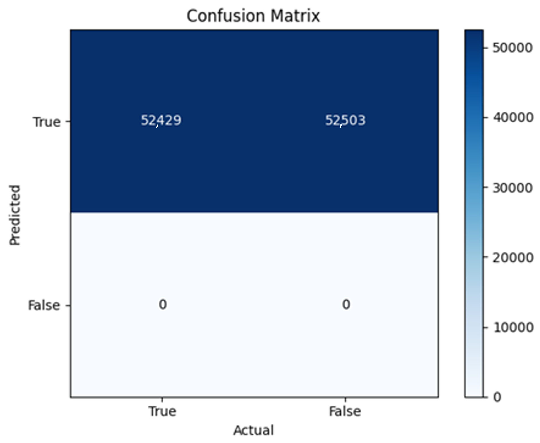
F3-Adam failed to converge and halted too early, resulting in increasing loss and decreasing accuracy over the course of 7 training epochs. Having TN and FN both equal 0 indicates that the model predicted all samples as the positive class (Fake accounts), which emphasizes the optimizer instability and sensitivity.
F3-RMSprop excels at detecting real accounts, with 91% specificity; however, it struggles with some fake accounts, as shown in the 6 ~ 7% recall, meaning that it misses around 33% of fake accounts. This can be seen by the relatively low number of 4742 FP (real accounts predicted as fake) compared to 35,017 TP (fake accounts predicted as fake).
Additionally, F3-SGD-LR (0.015) struggled to converge to a stable loss value and continuously fluctuated until early stopping intervened to halt the process.
Early stopping has also intervened with F3-SGD_LR (0.001) training, as the model was able to converge and learn for 58 epochs, resulting in a loss of 0.416 and an accuracy of 79%. Similarly, the F3-Adatelta model continued training for 196 epochs, achieving a comparable loss of 0.418 and the same accuracy.
Table A3 displays other favorable metrics for these two models. Both models exhibited similar values, with precision around 0.8, recall around 0.6, specificity of 0.9, and F1 and F2 scores approximately at 0.7. The Matthews correlation coefficient (MCC) was approximately 0.59 for both models. All the results and plots related to this model are summarized in Table A3, and confusion matrices can be found in the appendix (Figure A27Figure A32).
Table A3. F3 Results.
NameepochsAccLossAUCTPTNFPFNPrecisionRecallSpecificityF1F2MCC
F3-SGD150.790.4220.86735,00047,759474417,4290.8810.6680.910.7590.7020.595
F3-RMSprop80.790.4180.86735,01747,761474217,4120.8810.6680.910.760.9020.5953
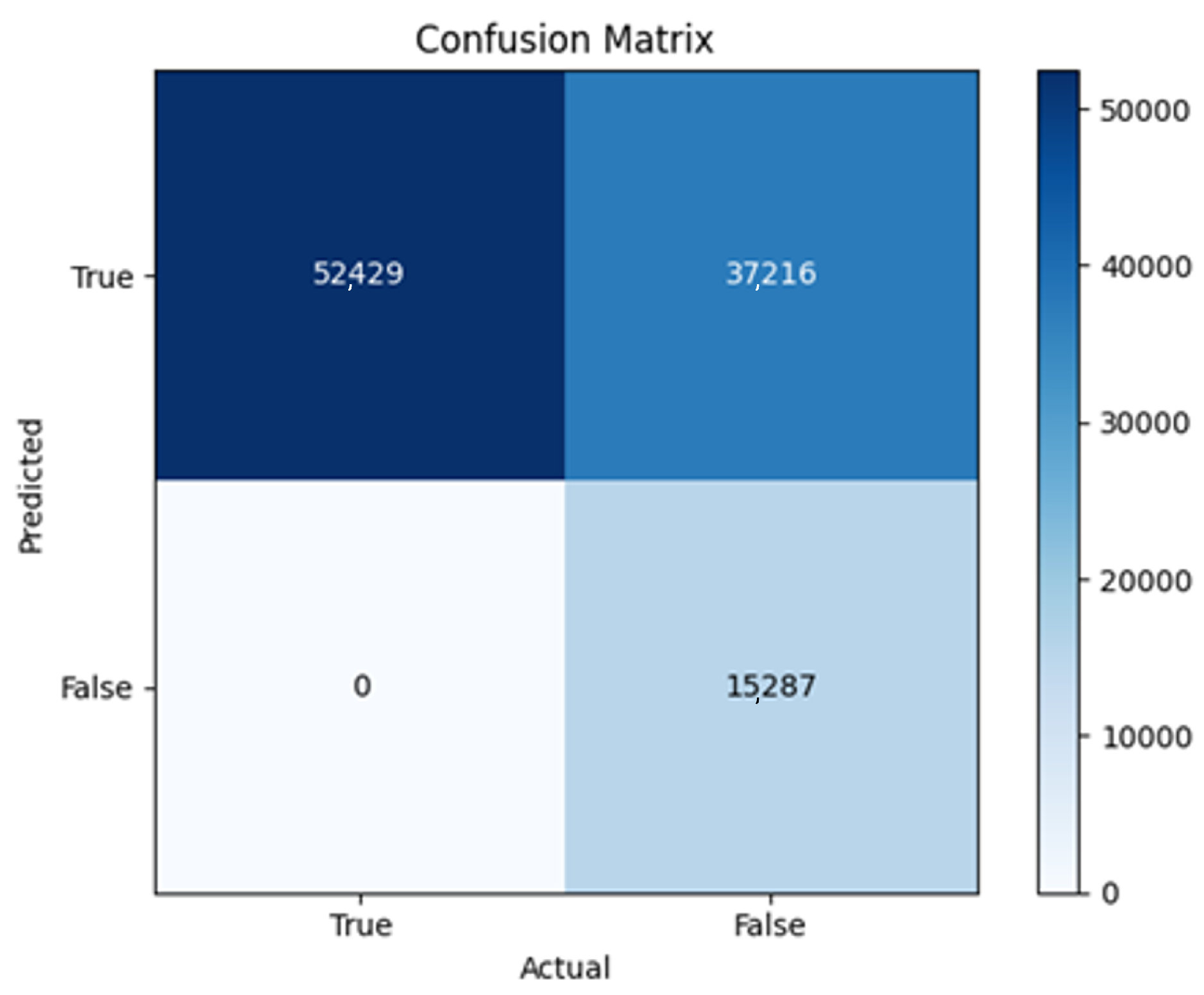
F3-Adam70.50.6930.552,429052,50300.5100.6660.833N/A
F3-Adadelta1960.790.4180.86735,01647,742476117,4130.880.6680.9090.760.7020.5949
F3-SGD-lr (0.015)140.790.4190.86834,98347,760474317,4460.8810.6670.910.760.7010.595
F3-SGD-lr (0.001)580.790.4190.86835,01747,760474317,4120.8810.6680.910.760.7020.5953

Appendix A.4. F-4 Model

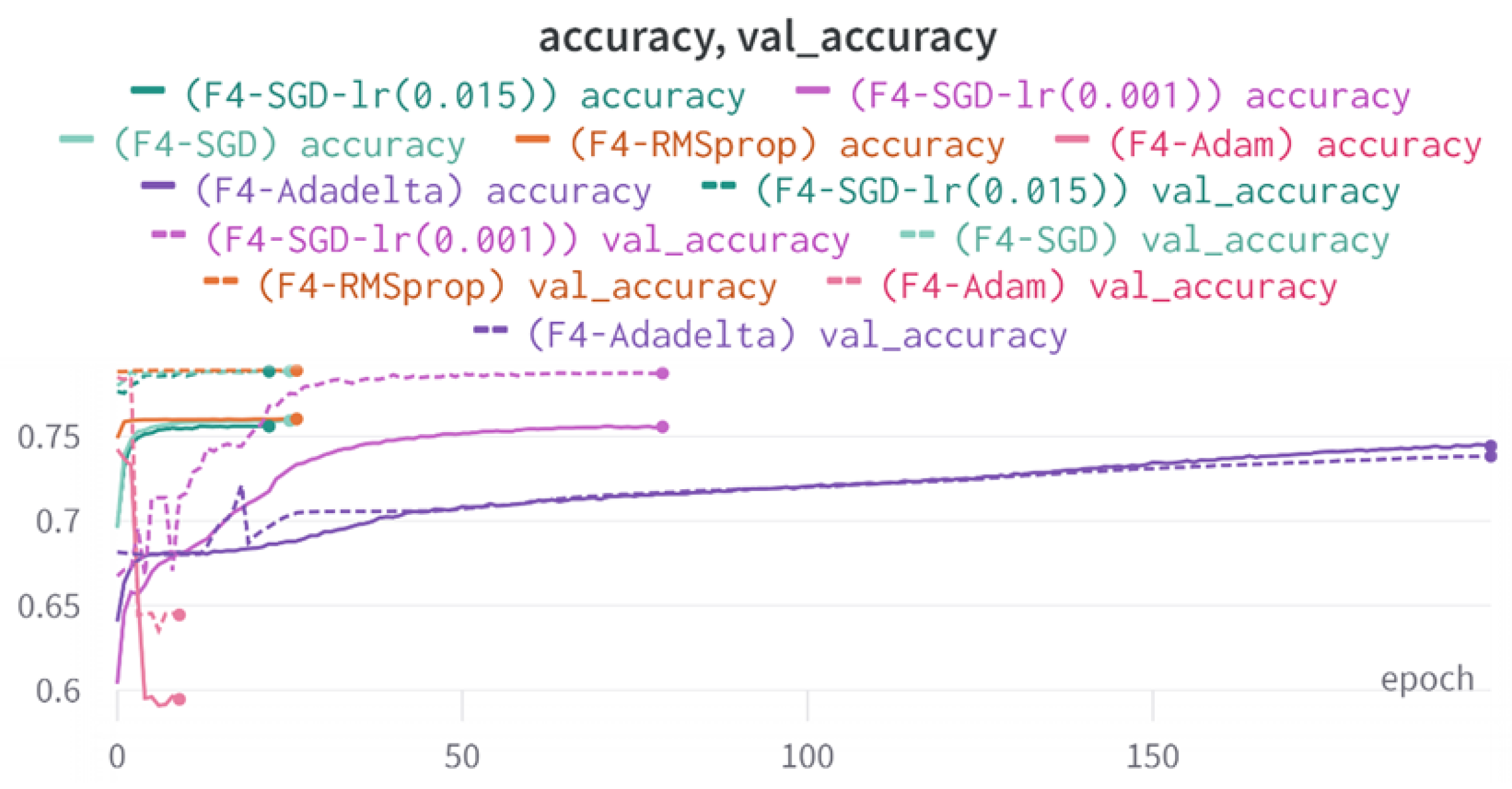
Out of the different optimizers of this architecture, only F4-Adadelta completed the 200 training epochs. Both F4-Adam and F4-RMSprop exhibited underfitting and failed to effectively learn from the data, as evidenced by their unstable curves as depicted in Figure A7 and Figure A8.
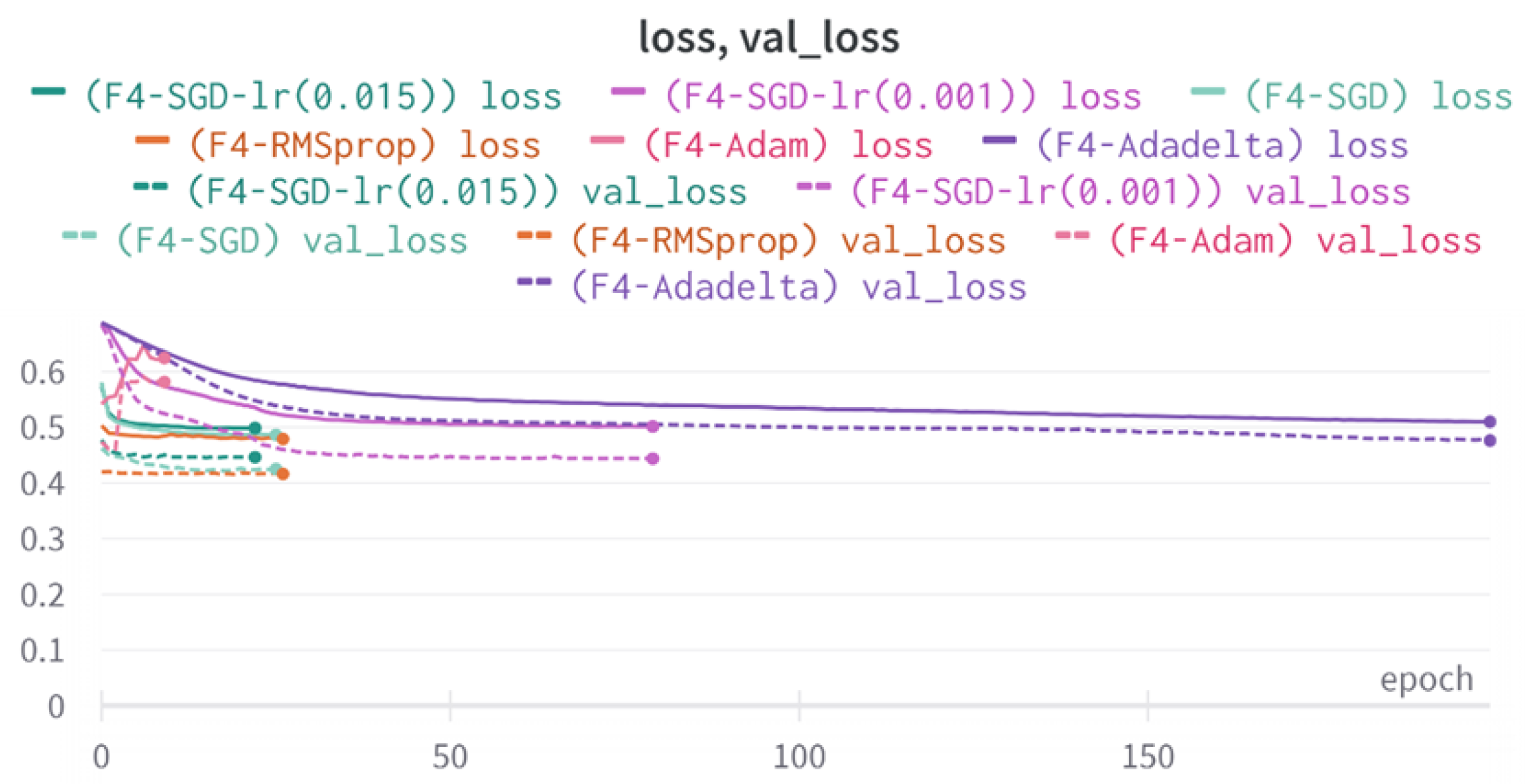
F4-SGD training was stopped after 25 epochs due to fluctuating loss and validation loss towards the end. On the other hand, F4-Adadelta completed the full 200 epochs but did not converge to a stable loss value. This indicates that further training and fine-tuning might be necessary, as both accuracy and loss did not stabilize. When using the learning rate reducer on the SGD optimizer with two different initial learning rate values of 0.001 and 0.015, it was observed that F4-SGD-LR (0.015) achieved faster convergence and reached a stable loss value earlier compared to F4-SGD-LR (0.001). The former model completed training after 22 epochs, while the latter model halted after 79 training epochs.
Figure A7. F4 models loss, validation loss.
Bdcc 09 00298 g0a7
Figure A8. F4 models accuracy, validation accuracy.
Bdcc 09 00298 g0a8
In terms of loss, F4-RMSprop achieved the lowest value of 0.416. Apart from F4-Adam, all models had a similar accuracy of approximately 79%. The learning rate was reduced to 0.00015 in F4-SGD-LR (0.015) and to 0.00001 in F4-SGD-LR (0.001). When considering the F1 and F2 scores, F4-Adadelta had the highest values, with 0.77 for the F1 score and 0.84 for the F2 score. However, when considering the Matthews Correlation Coefficient (MCC) and examining the confusion matrix, it is evident that F4-Adadelta may not be the best-performing model. Detailed results can be found in Table A4 and confusion matrices are available in the appendix from Figure A33Figure A38.
Table A4. F4 Results.
NameepochsAccLossAUCTPTNFPFNPrecisionRecallSpecificityF1F2MCC
F4-SGD250.790.4250.86834,98147,760474317,4480.8810.6670.910.760.7010.5947
F4-RMSprop260.790.4160.86835,01847,761474217,4110.8810.6680.910.760.7020.5953
F4-Adam90.640.5820.64552,42915,19737,30600.58610.2890.7380.8750.4112
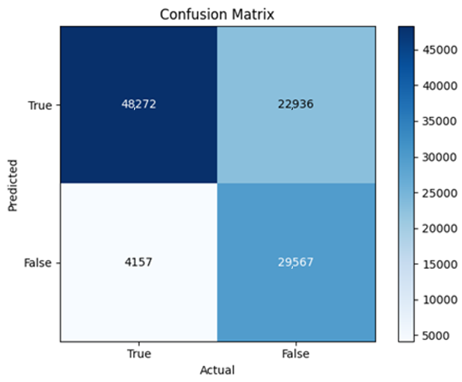
F4-Adadelta1990.740.4760.86146,88630,58121,92255430.6810.8940.5820.7730.8420.5017
F4-SGD-lr (0.015)220.790.4460.85534,96447,761474217,4650.8810.6670.910.7590.70.5944
F4-SGD-lr (0.001)790.790.4440.85434,84547,761474217,5840.880.6650.910.7570.6990.5924

Appendix A.5. 2B1 Model

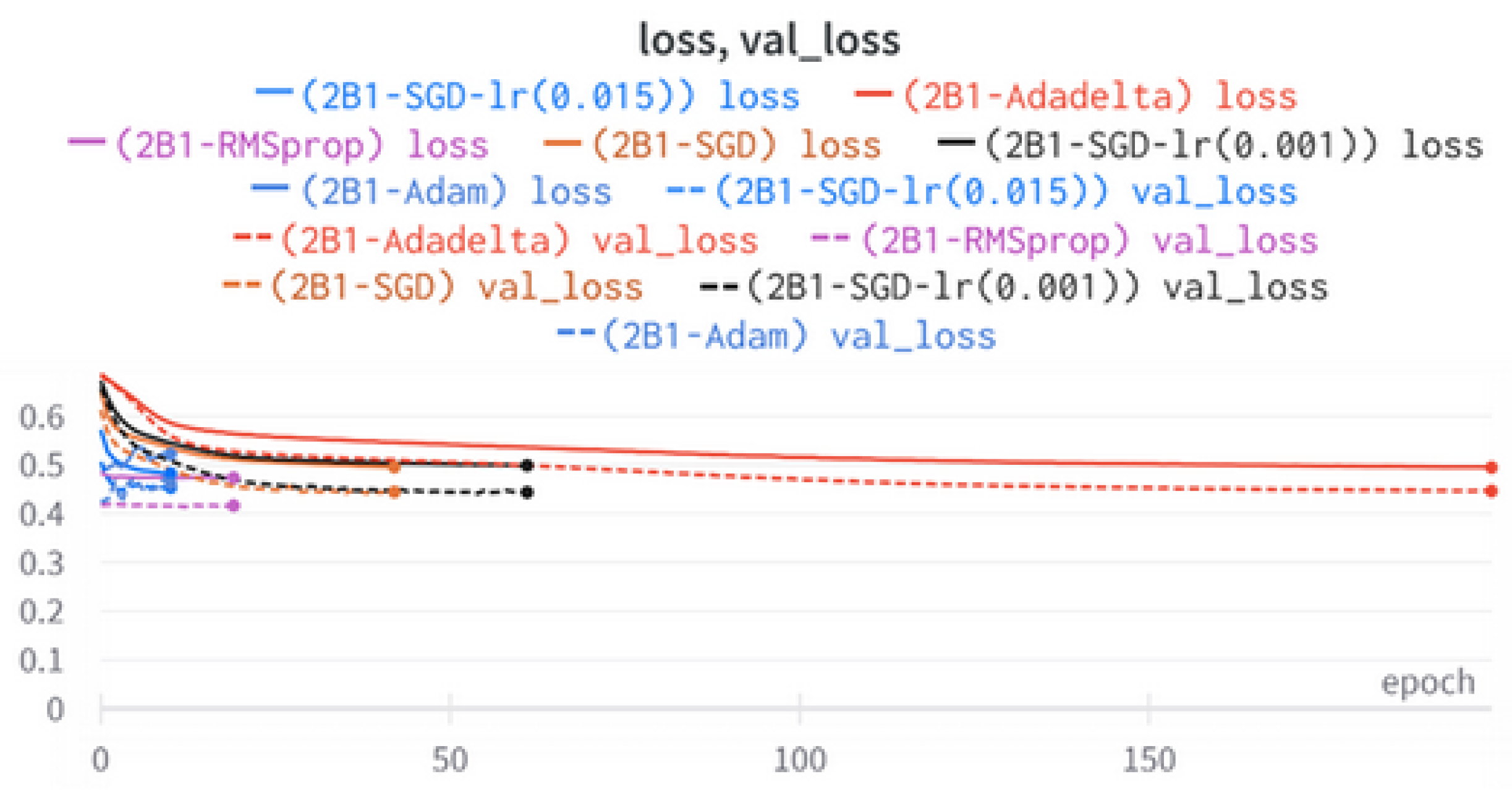
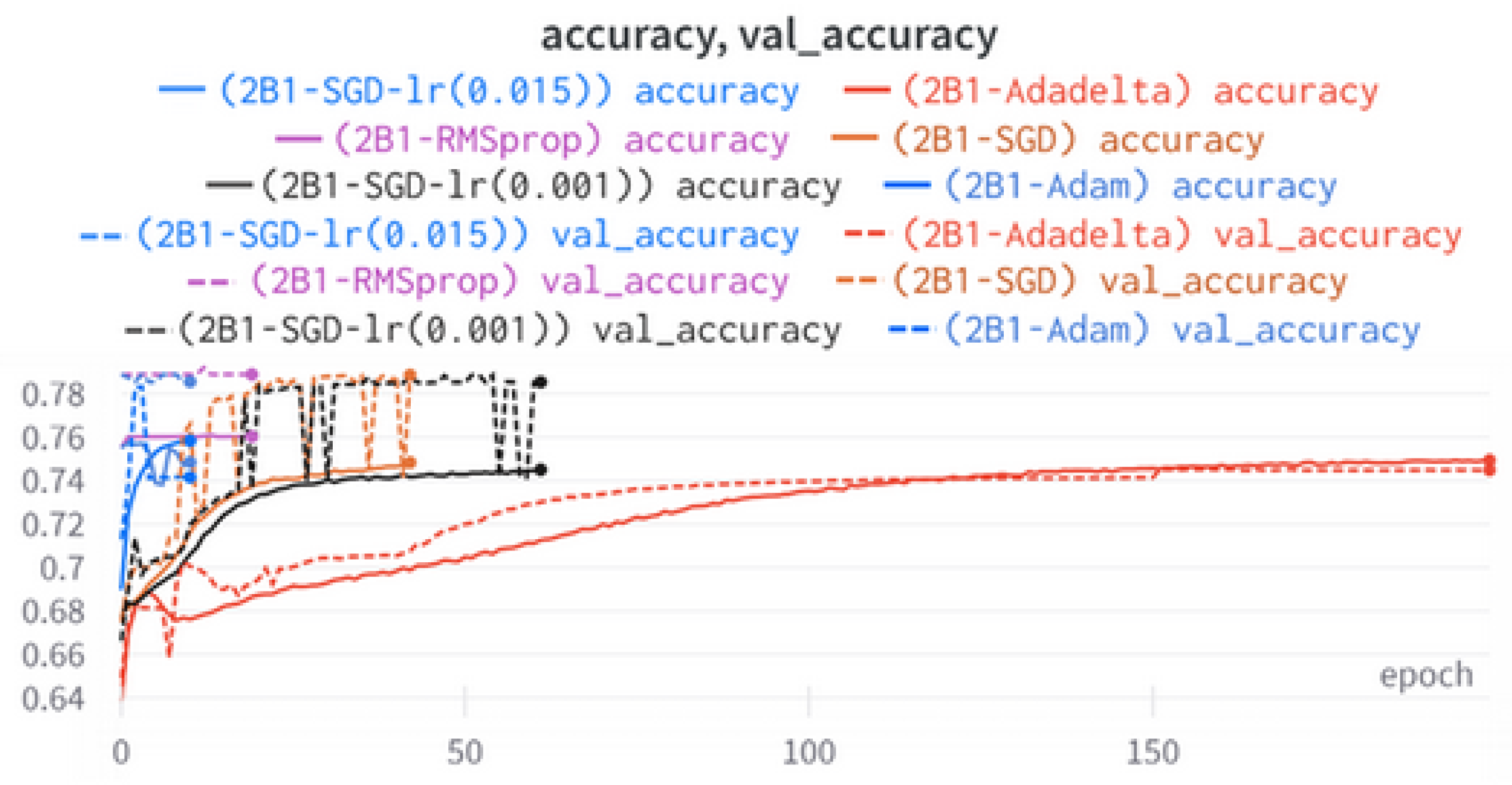
2B1-SGD halted after 42 epochs due to the presence of fluctuating validation loss and unstable accuracy.
Despite this, other metrics indicate good performance. On the other hand, both 2B1-RMSprop and 2B1-Adam exhibit clear signs of underfitting (Figure A9), suggesting that they were unable to adequately learn from the data. Even though 2B1-Adadelta obtained lower values, its performance demonstrates a better fit and learning from the data. However, it is worth noting that neither accuracy nor loss reached a stable level towards the end of training. Thus, Additional training and further fine-tuning might improve the model’s performance. When applying the learning rate reducer, the learning rate in 2B1-SGD-LR (0.015) reached around 0.0015 in an attempt to fit the data. However, these attempts were unsuccessful. Conversely, in 2B1-SGD-LR (0.001), the learning rate remained the same and resulted in a better fit to the data. Nevertheless, we can find a similar fluctuating behavior in the accuracy curve for this model (Figure A10).
Figure A9. 2B1 models loss, validation loss.
Bdcc 09 00298 g0a9
Figure A10. 2B1 models accuracy, validation accuracy.
Bdcc 09 00298 g0a10
All the results and evolution metrics for this model are demonstrated in Table A5, and confusion matrices are available in the appendix (Figure A39Figure A44).
Table A5. 2B1 Results.
NameepochsAccLossAUCTPTNFPFNPrecisionRecallSpecificityF1F2MCC
2B1-SGD420.790.4440.86634,99247,755474817,4370.8810.6670.910.7590.7010.5947
2B1-RMSprop190.790.4170.86835,01847,761474217,4110.8810.6680.910.760.7020.5953
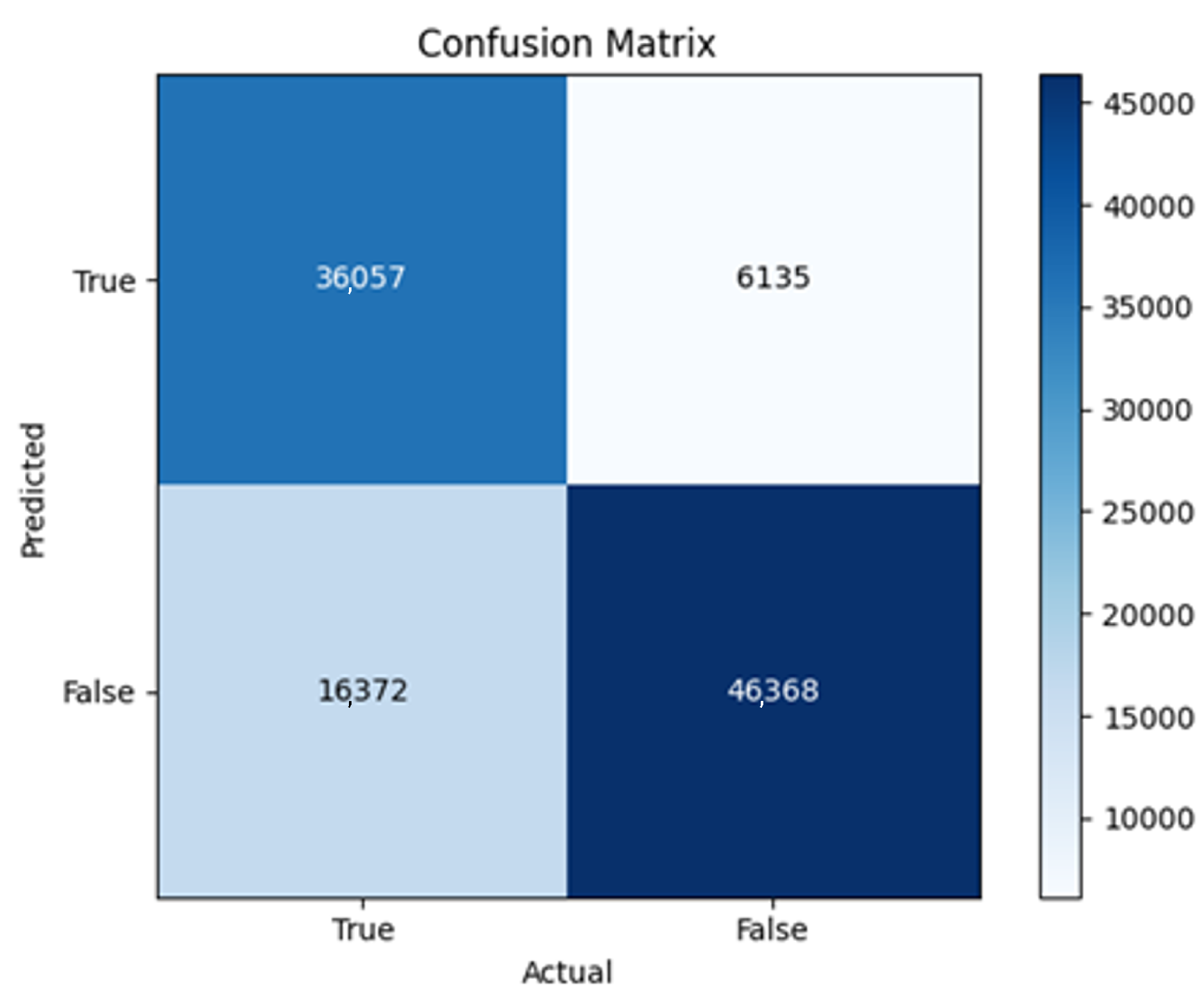
2B1-Adam100.790.4610.83136,05746,368613516,3720.8550.6880.8830.7620.7160.5822
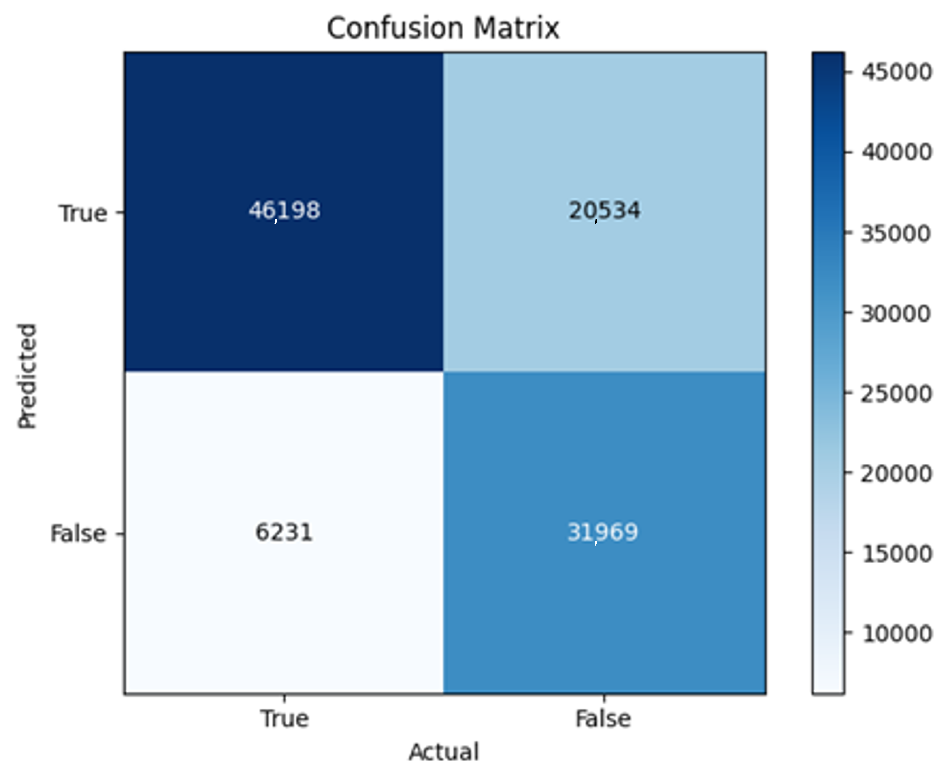
2B1-Adadelta1990.740.4460.86746,19831,96920,53462310.6920.8810.6090.7750.8360.5092
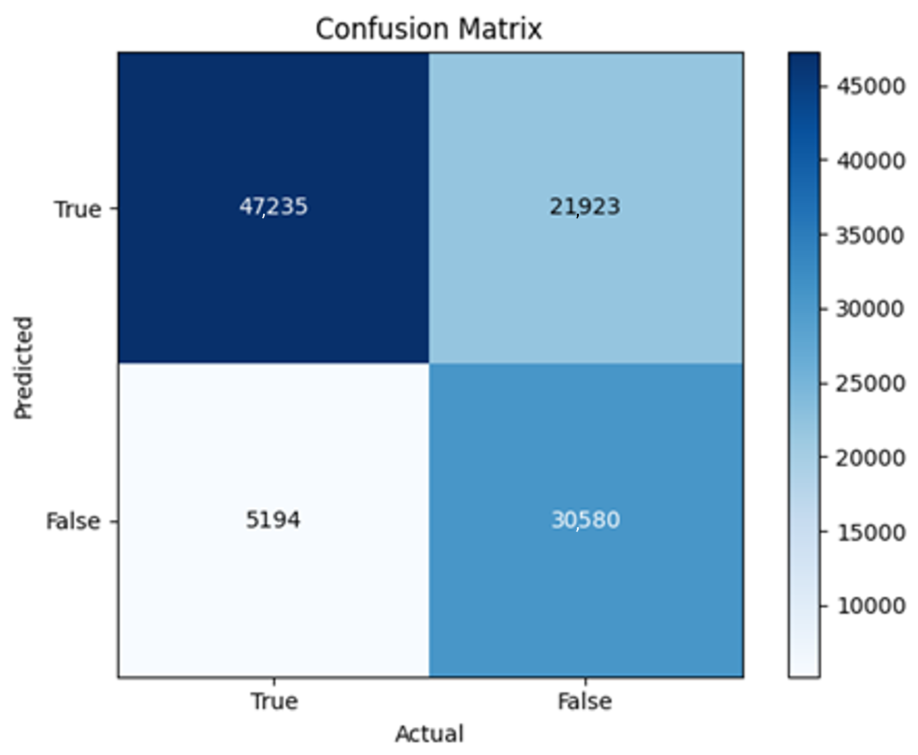
2B1-SGD-lr (0.015)100.740.4540.86847,23530,58021,92351940.6830.9010.5820.7770.8470.5099
2B1-SGD-lr (0.001)610.790.4440.86636,04246,366613716,3870.8550.6870.8830.7620.7150.5818

Appendix A.6. 2B2 Model

Among the examined 2B2 models, only 3 of them were able to effectively learn and converge: 2B2-SGD, 2B2-Adadelta, and 2B2-SGD-LR (0.001), the other 3 models showed some fluctuation and instability, which caused them to stop training before reaching the 10th epoch (Figure A11).
In terms of Accurracy, 2B2-SGD-LR (0.015) is the lowest with 7 ~ 4%, and 2B2-RMSprop acheived the highest accuracy of 80% (Figure A12).
In the case of 2B2-SGD-LR (0.001), the learning rate reducer dropped learning rate value to 0.000015.
Figure A11. 2B2 loss, validation loss.
Bdcc 09 00298 g0a11
Figure A12. 2B2 accuracy, validation accuracy.
Bdcc 09 00298 g0a12
2B2-Adadelta took the longest training time, halting after 106 epochs. When comparing these three models using various evaluation metrics listed in Table A6, it can be observed that they exhibit very similar values.
Table A6. 2B2 Results.
NameepochsAccLossAUCTPTNFPFNPrecisionRecallSpecificityF1F2MCC
2B2-SGD220.790.3920.88838,78744,532797113,6420.830.740.8480.7820.7560.5915
2B2-RMSprop80.80.3980.88638,90844,558794513,5210.830.7420.8490.7840.7580.5942
2B2-Adam70.790.4020.88839,02844,359814413,4010.8270.7440.8450.7840.760.5923
2B2-Adadelta1060.790.3940.88739,02044,281822213,4090.8260.7440.8430.7830.7590.5906
2B2-SGD-lr (0.015)100.740.4240.88448,27229,56722,93641570.6780.9210.5630.7810.860.518
2B2-SGD-lr (0.001)290.790.3940.88738,76244,508799513,6670.8290.7390.8480.7820.7560.5906
Looking at F1 and F2 scores, 2B2-Adadelta slightly outperformed the other models, achieving values of 0.782 and 0.759, respectively. All results related to this model are demonstrated in Table A6, and confusion matrix plots can be found in the appendix from Figure A45Figure A50.

Appendix A.7. 2B3 Model

Different runs on this architecture (Figure A13 and Figure A14) showed fluctuating behavior for both 2B3-RMSprop, and 2B3-Adam. The latter one shows a severe imbalance in its prediction. Detecting all fake accounts correctly (TP = 52,429, TN = 0), achieving 100% recall. However, the high false positive (FP = 37,216 real accounts flagged as fake) resulting in a low 58% precision, and low True negative (TN = 15,287 real accounts correctly predicted as real) suggest that this model is overly aggressive in labeling accounts as fake to avoid missing any true positives.
Figure A13. 2B3 loss, validation loss.
Bdcc 09 00298 g0a13
Figure A14. 2B3 accuracy, validation accuracy.
Bdcc 09 00298 g0a14
On the other hand, the 2B3 model with the SGD optimizer, both with and without the learning rate reducer, showed better balance and demonstrated a good fit with relatively high metrics. Among all the models proposed in this work and using different optimizers, the 2B3-SGD and 2B3-SGD-LR (0.015) achieved the highest MCC value (Table A7). In the 2B3-SGD-LR (0.015) model, while attempting to optimize the learning rate, the reducer decreased its value to 1.500000053056283 × 10⁻⁷. This change had an impact on the loss, reducing it to 0.413 instead of 0.414. There was a slight improvement in specificity. It is worth mentioning that these values were obtained by training for only 60 epochs instead of 69 without the reducer. The Adadelta optimizer also demonstrated high performance. The 2B3-Adadelta Model performed similarly to 2B3-SGD-LR (0.001) in most metrics, achieving a Precision of 0.88, Recall of 0.668, Specificity of 0.91, F1 score of 0.759, an F2 score of 0.702, and a MCC of 0.5947. All the results and plots related to this model are demonstrated in Table A7, and confusion matrices are in the appendix (from Figure A51Figure A56).
Table A7. 2B3 Results.
NameepochsAccLossAUCTPTNFPFNPrecisionRecallSpecificityF1F2MCC
2B3-SGD690.790.4140.8735,38647,727477617,0430.8810.6750.9090.7640.7080.6007
2B3-RMSprop120.790.4170.86835,01847,760474317,4110.8810.6680.910.760.7020.5953
2B3-Adam250.6450.4940.74752,42915,28737,21600.58510.2910.7380.8760.4127
2B3-Adadelta1990.790.4190.86835,01347,739476417,4160.880.6680.910.7590.7020.5947
2B3-SGD-lr (0.015)600.790.4130.8735,38747,726477717,0420.8810.6750.910.7640.7080.6007
2B3-SGD-lr (0.001)590.790.4190.86735,01147,748475517,4180.880.6680.910.760.7020.595

Appendix B. Confusion Matrices

Figure A15. F1-SGD Confusion matrix.
Bdcc 09 00298 g0a15
Figure A16. F1-RMSprop Confusion matrix.
Bdcc 09 00298 g0a16
Figure A17. F1-Adam Confusion matrix.
Bdcc 09 00298 g0a17
Figure A18. F1-Adadelta Confusion matrix.
Bdcc 09 00298 g0a18
Figure A19. F1-SGD-LR (0.015) Confusion matrix.
Bdcc 09 00298 g0a19
Figure A20. F1-SGD-LR (0.001) Confusion matrix.
Bdcc 09 00298 g0a20
Figure A21. F2-SGD Confusion Matrix.
Bdcc 09 00298 g0a21
Figure A22. F2-RMSprop Confusion Matrix.
Bdcc 09 00298 g0a22
Figure A23. F2-Adam Confusion Matrix.
Bdcc 09 00298 g0a23
Figure A24. F2-Adadelta Confusion Matrix.
Bdcc 09 00298 g0a24
Figure A25. F2-SGD-LR (0.015) Confusion Matrix.
Bdcc 09 00298 g0a25
Figure A26. F2-SGD-LR (0.001) Confusion Matrix.
Bdcc 09 00298 g0a26
Figure A27. F3-SGD Confusion Matrix.
Bdcc 09 00298 g0a27
Figure A28. F3-RMSprop Confusion Matrix.
Bdcc 09 00298 g0a28
Figure A29. F3-Adam Confusion Matrix.
Bdcc 09 00298 g0a29
Figure A30. F3-Adadelta Confusion Matrix.
Bdcc 09 00298 g0a30
Figure A31. F3-SGD-LR (0.015) Confusion Matrix.
Bdcc 09 00298 g0a31
Figure A32. F3-SGD-LR (0.001) Confusion Matrix.
Bdcc 09 00298 g0a32
Figure A33. F4-SGD Confusion Matrix.
Bdcc 09 00298 g0a33
Figure A34. F4-RMSprop Confusion Matrix.
Bdcc 09 00298 g0a34
Figure A35. F4-Adam Confusion Matrix.
Bdcc 09 00298 g0a35
Figure A36. F4-Adadelta Confusion Matrix.
Bdcc 09 00298 g0a36
Figure A37. F4-SGD-LR (0.015) Confusion Matrix.
Bdcc 09 00298 g0a37
Figure A38. F4-SGD-LR (0.001) Confusion Matrix.
Bdcc 09 00298 g0a38
Figure A39. 2B1-SGD Confusion Matrix.
Bdcc 09 00298 g0a39
Figure A40. 2B1-RMSprop Confusion Matrix.
Bdcc 09 00298 g0a40
Figure A41. 2B1-Adam Confusion Matrix.
Bdcc 09 00298 g0a41
Figure A42. 2B1-Adadelta Confusion Matrix.
Bdcc 09 00298 g0a42
Figure A43. 2B1-SGD-LR (0.015) Confusion Matrix.
Bdcc 09 00298 g0a43
Figure A44. 2B1-SGD-LR (0.001) Confusion Matrix.
Bdcc 09 00298 g0a44
Figure A45. 2B2-SGD Confusion Matrix.
Bdcc 09 00298 g0a45
Figure A46. 2B2-RMSprop Confusion Matrix.
Bdcc 09 00298 g0a46
Figure A47. 2B2-Adam Confusion Matrix.
Bdcc 09 00298 g0a47
Figure A48. 2B2-Adadelta Confusion Matrix.
Bdcc 09 00298 g0a48
Figure A49. 2B2-SGD-LR (0.015) Confusion Matrix.
Bdcc 09 00298 g0a49
Figure A50. 2B2-SGD-LR (0.001) Confusion Matrix.
Bdcc 09 00298 g0a50
Figure A51. 2B3-SGD Confusion Matrix.
Bdcc 09 00298 g0a51
Figure A52. 2B3-RMSprop Confusion Matrix.
Bdcc 09 00298 g0a52
Figure A53. 2B3-Adam Confusion Matrix.
Bdcc 09 00298 g0a53
Figure A54. 2B3-Adadelta Confusion Matrix.
Bdcc 09 00298 g0a54
Figure A55. 2B3-SGD-LR (0.015) Confusion Matrix.
Bdcc 09 00298 g0a55
Figure A56. 2B3-SGD-LR (0.001) Confusion Matrix.
Bdcc 09 00298 g0a56

Appendix C. Model Summaries

Figure A57. F-1 model summary.
Bdcc 09 00298 g0a57
Figure A58. F-2 model summary.
Bdcc 09 00298 g0a58
Figure A59. F-3 model summary.
Bdcc 09 00298 g0a59
Figure A60. F-4 model summary.
Bdcc 09 00298 g0a60
Figure A61. 2B1 model summary.
Bdcc 09 00298 g0a61
Figure A62. 2B2 model summary.
Bdcc 09 00298 g0a62

References

  1. Keles, B.; McCrae, N.; Grealish, A. A systematic review: The influence of social media on depression, anxiety and psychological distress in adolescents. Int. J. Adolesc. Youth 2020, 25, 79–93. [Google Scholar] [CrossRef]
  2. Akram, W.; Kumar, R. A study on positive and negative effects of social media on society. Int. J. Comput. Sci. Eng. 2017, 5, 351–354. [Google Scholar] [CrossRef]
  3. Song, J.; Lee, S.; Kim, J. Crowdtarget: Target-based detection of crowdturfing in online social networks. In Proceedings of the 22nd ACM SIGSAC Conference on Computer and Communications Security, Denver, CO, USA, 12–16 October 2015; pp. 793–804. [Google Scholar]
  4. Benevenuto, F.; Magno, G.; Rodrigues, T.; Almeida, V. Detecting spammers on twitter. In Proceedings of the Collaboration, Electronic Messaging, Anti-Abuse and Spam Conference (CEAS), Redmond, WA, USA, 13–14 July 2010; Volume 6, p. 12. [Google Scholar]
  5. Romanov, A.; Semenov, A.; Mazhelis, O.; Veijalainen, J. Detection of fake profiles in social media. In Proceedings of the 13th International Conference on Web Information Systems and Technologies (WEBIST 2017), Porto, Portugal, 25–27 April 2017; pp. 363–369. [Google Scholar]
  6. Gurajala, S.; White, J.S.; Hudson, B.; Matthews, J.N. Fake Twitter accounts: Profile characteristics obtained using an activity-based pattern detection approach. In Proceedings of the 2015 International Conference on Social Media & Society, Toronto, ON, Canada, 27–29 July 2015; pp. 1–7. [Google Scholar]
  7. Nazir, A.; Raza, S.; Chuah, C.N.; Schipper, B. Ghostbusting facebook: Detecting and characterizing phantom profiles in online social gaming applications. In Proceedings of the 3rd Workshop on Online Social Networks (WOSN 2010), Boston, MA, USA, 22 June 2010. [Google Scholar]
  8. Andriopoulou, F.; Mavromatis, G.; Katsaros, D. Fake account detection in online social networks using graph-based features and ensemble learning. J. Netw. Comput. Appl. 2018, 121, 1–12. [Google Scholar]
  9. Idir, M.A.; Hassouni, M.E.; Ouanan, M. Fake accounts detection in online social networks using graph-based features. Int. J. Adv. Comput. Sci. Appl. 2016, 7, 215–222. [Google Scholar]
  10. Cao, Y.; Li, W.; Zhang, J. Real-time traffic information collecting and monitoring system based on the internet of things. In Proceedings of the 2011 6th International Conference on Pervasive Computing and Applications, Oulu, Finland, 11–13 May 2011; IEEE: Piscataway, NJ, USA, 2011; pp. 45–49. [Google Scholar]
  11. Boshmaf, Y.; Logothetis, D.; Siganos, G.; Lería, J.; Lorenzo, J.; Ripeanu, M.; Beznosov, K. Íntegro: Leveraging victim prediction for robust fake account detection in large scale OSNs. Comput. Secur. 2016, 61, 142–168. [Google Scholar] [CrossRef]
  12. Egele, M.; Stringhini, G.; Kruegel, C.; Vigna, G. Towards detecting compromised accounts on social networks. IEEE Trans. Dependable Secur. Comput. 2015, 14, 447–460. [Google Scholar] [CrossRef]
  13. Stringhini, G.; Wang, G.; Egele, M.; Kruegel, C.; Vigna, G.; Zheng, H.; Zhao, B.Y. Follow the green: Growth and dynamics in twitter follower markets. In Proceedings of the 2013 Conference on Internet Measurement Conference, Barcelona, Spain, 23–25 October 2013; pp. 163–176. [Google Scholar]
  14. Wang, G.; Wilson, C.; Zhao, X.; Zhu, Y.; Mohanlal, M.; Zheng, H.; Zhao, B.Y. Serf and turf: Crowdturfing for fun and profit. In Proceedings of the 21st International Conference on World Wide Web, Lyon, France, 16–20 April 2012; pp. 679–688. [Google Scholar]
  15. Wang, G.; Wang, T.; Zheng, H.; Zhao, B.Y. Man vs. machine: Practical adversarial detection of malicious crowdsourcing workers. In Proceedings of the 23rd USENIX Security Symposium (USENIX Security 14), San Diego, CA, USA, 20–22 August 2014; pp. 239–254. [Google Scholar]
  16. Yuan, D.; Miao, Y.; Gong, N.; Yang, Z.; Li, Q.; Song, D.; Wang, Q.; Liang, X. Detecting fake accounts in online social networks at the time of registrations. In Proceedings of the 2019 ACM SIGSAC Conference on Computer and Communications Security, London, UK, 11–15 November 2019; pp. 1423–1438. [Google Scholar]
  17. Lee, K.; Caverlee, J.; Webb, S. Uncovering Social Spammers: Social Honeypots + Machine Learning. In Proceedings of the 19th ACM International Conference on Information and Knowledge Management, ACM, Toronto, ON, Canada, 26–30 October 2010; pp. 435–442. [Google Scholar]
  18. Lee, K.; Eoff, B.; Caverlee, J. Seven Months with the Devils: A Long-Term Study of Content Polluters on Twitter. In Proceedings of the 5th International AAAI Conference on Weblogs and Social Media (ICWSM), Barcelona, Spain, 17–21 July 2011. [Google Scholar]
  19. Crescia, S.; DiPietro, R.; Petrocchi, M.; Spognardi, A.; Tesconi, M. Fame for Sale: Efficient Detection of Fake Twitter Followers. Decis. Support Syst. 2015, 80, 56–71. [Google Scholar] [CrossRef]
  20. Chen, C.; Zhang, J.; Chen, X.; Xiang, Y.; Zhou, W. 6 Million Spam Tweets: A Large Ground Truth for Timely Twitter Spam Detection. In Proceedings of the 2015 IEEE International Conference on Communications (ICC), London, UK, 8–12 June 2015; pp. 7065–7070. [Google Scholar]
  21. Gowda, S.R.S.; Archana, B.R.; Shettigar, P.; Satyarthi, K.K. Sentiment Analysis of Twitter Data Using Naïve Bayes Classifier. In ICDSMLA 2020; Kumar, A., Senatore, S., Gunjan, V.K., Eds.; Lecture Notes in Electrical Engineering; Springer: Singapore, 2022; Volume 783. [Google Scholar] [CrossRef]
  22. Fazil, M.; Abulaish, M. A Hybrid Approach for Detecting Automated Spammers in Twitter. IEEE Trans. Inf. Forensics Secur. 2018, 13, 2707–2719. [Google Scholar] [CrossRef]
  23. Yang, C.; Harkreader, R.; Gu, G. Empirical evaluation and new design for fighting evolving Twitter spammers. IEEE Trans. Inf. Forensics Secur. 2013, 8, 1280–1293. [Google Scholar] [CrossRef]
  24. Wu, T.; Liu, S.; Zhang, J.; Xiang, Y. Twitter Spam Detection Based on Deep Learning. In Proceedings of the ACSW 2017: Australasian Computer Science Week 2017, Geelong, Australia, 30 January–3 February 2017; pp. 1–8. [Google Scholar]
  25. Alom, Z.; Carminati, B.; Ferrari, E. A deep learning model for Twitter spam detection. Online Soc. Netw. Media 2020, 18, 100079. [Google Scholar] [CrossRef]
  26. Liu, Y.; Tan, Z.; Wang, H.; Feng, S.; Zheng, Q.; Luo, M. BotMoE: Twitter Bot Detection with Community-Aware Mixtures of Modal-Specific Experts. In Proceedings of the SIGIR ’23: The 46th International ACM SIGIR Conference on Research and Development in Information Retrieval, Taipei, Taiwan, 23–27 July 2023; pp. 485–495. [Google Scholar]
  27. Feng, S.; Tan, Z.; Wan, H.; Wang, N.; Chen, Z.; Zhang, B.; Zheng, Q.; Zhang, W.; Lei, Z.; Yang, S.; et al. Twibot-22: Towards Graph-Based Twitter Bot Detection. Adv. Neural Inf. Process. Syst. 2022, 35, 35254–35269. [Google Scholar]
  28. Shevtsov, A.; Antonakaki, D.; Lamprou, I.; Pratikakis, P.; Ioannidis, S. BotArtist: Generic Approach for Bot Detection in Twitter via Semi-Automatic Machine Learning Pipeline. arXiv 2023, arXiv:2306.00037v5. [Google Scholar]
  29. Alghamdi, M.A.; Quijano-Sanchez, L.; Liberatore, F. Enhancing Misinformation Countermeasures: A Multimodal Approach to Twitter Bot Detection. Soc. Netw. Anal. Min. 2025, 15, 1–20. [Google Scholar] [CrossRef]
  30. Kamiński, K.; Sepczuk, M. Detecting Fake Accounts on Social Media Portals—The X Portal Case Study. Electronics 2024, 13, 2542. [Google Scholar] [CrossRef]
  31. Zouzou, Y.; Varol, O. Unsupervised detection of coordinated fake-follower campaigns on social media. EPJ Data Sci. 2024, 13, 62. [Google Scholar] [CrossRef]
  32. Kenny, R.; Fischhoff, B.; Davis, A.; Carley, K.M.; Canfield, C. Duped by bots: Why some are better than others at detecting fake social media personas. Hum. Factors 2024, 66, 88–102. [Google Scholar] [CrossRef] [PubMed]
  33. Ng, L.H.X.; Carley, K.M. A Global Comparison of Social Media Bot and Human Characteristics. Sci. Rep. 2025, 15, 10973. [Google Scholar] [CrossRef]
  34. Ferrara, E. Twitter spam and false accounts prevalence, detection, and characterization: A survey. First Monday 2022, 27. [Google Scholar] [CrossRef]
  35. Feng, S.; Wan, H.; Wang, N.; Li, J.; Luo, M. Twibot-20: A comprehensive twitter bot detection benchmark. In Proceedings of the 30th ACM International Conference on Information & Knowledge Management, Virtual, 26 October 2021; pp. 4485–4494. [Google Scholar]
  36. Gilani, Z.; Farahbakhsh, R.; Tyson, G.; Wang, L.; Crowcroft, J. Of bots and humans (on twitter). In Proceedings of the 2017 IEEE/ACM International Conference on Advances in Social Networks Analysis and Mining 2017, Sydney, Australia, 31 July 2017; pp. 349–354. [Google Scholar]
  37. Yang, K.C.; Varol, O.; Hui, P.M.; Menczer, F. Scalable and generalizable social bot detection through data selection. In Proceedings of the AAAI Conference on Artificial Intelligence, Philadelphia, PA, USA, 3 April 2020; Volume 34, No. 01. pp. 1096–1103. [Google Scholar]
  38. Cresci, S.; Di Pietro, R.; Petrocchi, M.; Spognardi, A.; Tesconi, M. Social fingerprinting: Detection of spambot groups through DNA-inspired behavioral modeling. IEEE Trans. Dependable Secur. Comput. 2017, 15, 561–576. [Google Scholar] [CrossRef]
  39. Cresci, S.; Lillo, F.; Regoli, D.; Tardelli, S.; Tesconi, M. $ FAKE: Evidence of spam and bot activity in stock microblogs on Twitter. In Proceedings of the International AAAI Conference on Web and Social Media, Palo Alto, CA, USA, 15 June 2018; Volume 12. No. 1. [Google Scholar]
  40. Mazza, M.; Cresci, S.; Avvenuti, M.; Quattrociocchi, W.; Tesconi, M. Rtbust: Exploiting temporal patterns for botnet detection on twitter. In Proceedings of the 10th ACM Conference on Web Science, Boston, MA, USA, 26 June 2019; pp. 183–192. [Google Scholar]
  41. Honnibal, M.; Montani, I. spaCy: Industrial-strength Natural Language Processing in Python, Version 2. Available online: https://spacy.io (accessed on 11 November 2025).
  42. Iglesias, F.; Zseby, T. Tabular and latent space synthetic data generation: A literature review. J. Big Data 2023, 10, 115. [Google Scholar] [CrossRef]
  43. Google Colab Development Team. Google Colab Notebook. 2024. Available online: https://colab.research.google.com/drive/1RX1UV4C6GR-0bVHD-6x2upCfKZghi3BW?usp=sharing (accessed on 11 November 2025).
  44. Weights and Biases Project. WandB. 2023. Available online: https://wandb.ai (accessed on 11 November 2025).
  45. Keras. Keras: SGD Optimizer; Year. Available online: https://keras.io/api/optimizers/sgd/ (accessed on 11 November 2025).
  46. Keras. RMSprop Optimizer; Year. Keras API Documentation. Available online: https://keras.io/api/optimizers/rmsprop/ (accessed on 11 November 2025).
  47. Keras Documentation. Adam Optimizer-Keras API. 2023. Available online: https://keras.io/api/optimizers/adam/ (accessed on 11 November 2025).
  48. Keras Documentation. AdaDelta Optimizer-Keras Documentation. 2023. Available online: https://keras.io/api/optimizers/adadelta/ (accessed on 11 November 2025).
  49. Keras. ReduceLROnPlateau Callback; Year of Access. Available online: https://keras.io/api/callbacks/reduce_lr_on_plateau/ (accessed on 11 November 2025).
  50. Keras. EarlyStopping; Year of Access. Available online: https://keras.io/api/callbacks/early_stopping/ (accessed on 11 November 2025).
  51. Grandini, M.; Bagli, E.; Visani, G. Metrics for multi-class classification: An overview. arXiv 2020, arXiv:2008.05756. [Google Scholar]
  52. Hossin, M.; Sulaiman, M. A Review on Evaluation Metrics for Data Classification Evaluations. Int. J. Data Min. Knowl. Manag. Process 2015, 5, 1–11. [Google Scholar] [CrossRef]
  53. Goodfellow, I.; Bengio, Y.; Courville, A. Deep Learning; MIT Press: Cambridge, MA, USA, 2016. [Google Scholar]
  54. OpenAI. Dense Layer-Keras API. Available online: https://keras.io/api/layers/core_layers/dense/ (accessed on 11 November 2025).
  55. Baldi, P.; Sadowski, P.J. Understanding dropout. In Proceedings of the Advances in Neural Information Processing Systems Volume 26, Lake Tahoe, NV, USA, 5–10 December 2013. [Google Scholar]
  56. Shrestha, A.; Mahmood, A. Review of Deep Learning Algorithms and Architectures. IEEE Access 2019, 7, 53040–53065. [Google Scholar] [CrossRef]
  57. Hernández-García, A.; König, P. Do Deep Nets Really Need Weight Decay and Dropout? arXiv 2018, arXiv:1802.07042. [Google Scholar]
  58. Gu, A.; Dao, T. Mamba: Linear-time sequence modeling with selective state spaces. In Proceedings of the First Conference on Language Modeling (COLM 2024), Philadelphia, PA, USA, 7–9 October 2024. [Google Scholar]
  59. Li, D.; Tan, S.; Zhang, Y.; Jin, M.; Pan, S.; Okumura, M.; Jiang, R. Dyg-mamba: Continuous state space modeling on dynamic graphs. arXiv 2024, arXiv:2408.06966. [Google Scholar]
  60. Li, D.; Kosugi, S.; Zhang, Y.; Okumura, M.; Xia, F.; Jiang, R. Revisiting dynamic graph clustering via matrix factorization. In Proceedings of the ACM on Web Conference 2025, Sydney, NSW, Australia, 22 April 2025; pp. 1342–1352. [Google Scholar]
  61. Li, D.; Ma, X.; Gong, M. Joint learning of feature extraction and clustering for large-scale temporal networks. IEEE Trans. Cybern. 2021, 53, 1653–1666. [Google Scholar] [CrossRef]
  62. Chen, Y.; Feng, L.; Zheng, C.; Zhou, T.; Liu, L.; Liu, P.; Chen, Y. LDANet: Automatic lung parenchyma segmentation from CT images. Comput. Biol. Med. 2023, 155, 106659. [Google Scholar] [CrossRef]
  63. Al Said, N. A Hybrid GAN-CNN Network with Attention Mechanism for Detecting Fake Profile Images in Microblogs. Ing. Des Syst. D’Information 2025, 30, 1447. [Google Scholar] [CrossRef]
Figure 1. Block diagram of the main components of the developed methodology.
Bdcc 09 00298 g001
Figure 2. Attributes in users.csv.
Bdcc 09 00298 g002
Figure 3. Attributes in followers.csv.
Bdcc 09 00298 g003
Figure 4. Attributes in tweets.csv.
Bdcc 09 00298 g004
Figure 5. Attributes in friends.csv.
Bdcc 09 00298 g005
Figure 6. Sample of legitimate users tweets.txt.
Bdcc 09 00298 g006
Figure 7. Sample of content polluters tweets.txt.
Bdcc 09 00298 g007
Figure 8. F-1 model architecture.
Bdcc 09 00298 g008
Figure 9. F-2 model architecture.
Bdcc 09 00298 g009
Figure 10. F-3 model architecture.
Bdcc 09 00298 g010
Figure 11. F-4 model architecture.
Bdcc 09 00298 g011
Figure 12. 2B1 model architecture.
Bdcc 09 00298 g012
Figure 13. 2B2 model architecture.
Bdcc 09 00298 g013
Table 1. Comparative Overview of State-of-the-Art Methods and Proposed Work.
ReferenceMethod UsedDatasetMetrics/Results
This WorkHybrid Deep Learning (Dense + LSTM)Fame for Sale [19], Social Honeypot [18] + (Augmented data)Overall - Acc: ≈79%, MCC: ≈0.6. Other reported metrics(Loss, AUC, confusion matrix, Precision, Recall, Specificity, F1/F2 scores)
 [26]Mixture of Experts with Graph Neural NetworksFame for Sale [19], TwiBot-20 [35], TwiBot-22 [27]highest: Acc: 98.5%, F1-Score: 89.22
[29]Community-aware Graph AnalysisTwiBot-22 [27]Acc: ≈0.90, F1-Score: ≈0.77
[28]Semi-Automatic ML Pipeline focused exclusively on lightweight user profile features9 Public datasets: [19,27,35,36,37,38,39,40]83.19% average F1-score in specific evaluations and the  10% improvement in general evaluation. All remaining performance is available in the original paper [28] Tables 3 and 4.
[30]Visual classification of X portal profiles using a CNNSynthetic generated image datasetBest: Acc: 96.5, Avg. Precision: 96.59, Avg. Recall: 96.40, Avg. F1-Score: 96.49
[31]Sliding Histogram is used to detect coordinated follower groups using anomaly scores.Synthetic datasetAverage Precision: ≈0.71, AUC: ≈0.87
[22]A hybrid ML using metadata, content, interaction, and community-based features with several classifiers.Twitter dataset [23]. Consists of 11k labeled users (10k benign/1k spammers)Reported metrics: Recall, False Positive Rate, F-score. Random Forest achieves the best overall performance.
Table 2. Distribution of the dataset used in the study.
Train SamplesTest Samples
Processed Dataset299,72674,932
Augmented Dataset70,00030,000
Final Dataset (Sum)369,726104,932
LabelsLabels
(0) 184,826(1) 184,900(0) 52,503(1) 52,429
Table 3. Statistics of dataset 1. Adapted from [19].
Relationships
DatasetTweetsFollowersFriendsTotal
TFP (@TheFakeProject)563,693258,494241,710500,204
E13 (#elezioni2013)2,068,0371,526,944667,2252,194,169
FSF (fastfollowerz)22,91011,893253,026264,919
INT (intertwitter)58,92523,173517,485540,658
TWT (twittertechnology)114,19228,588729,839758,427
HUM (human dataset)2,631,7301,785,438908,9352,694,373
FAK (fake dataset)118,32734,553879,580914,133
BAS (baseline dataset: HUM U FAK)2,750,0571,819,9911,788,5153,608,506
Note: This table reports statistics of the original source datasets and was not used directly for training; it is provided for context on data provenance.
Disclaimer/Publisher’s Note: The statements, opinions and data contained in all publications are solely those of the individual author(s) and contributor(s) and not of MDPI and/or the editor(s). MDPI and/or the editor(s) disclaim responsibility for any injury to people or property resulting from any ideas, methods, instructions or products referred to in the content.